
Время на прочтение
3 мин
Количество просмотров 21K
Доброго времени суток, в этой статье хочу рассказать о своём опыте работы с BI Publisher и составлении шаблонов для MS Excel в родном для этой программы формате *.xls.
Небольшое предисловие
Работая с Oracle eBS, время от времени возникает необходимость создания дополнительных репортов (а соответственно и шаблонов в BI Publisher). В данном случае был довольно сложный репорт, который собирался из таблиц, заполняющихся данными в BEFORE REPORT триггере этого же репорта. Количество колонок в репорте могло динамичиски меняться.
Первоначально шаблон был сделан в формате RTF. Для каждого количества колонок был предусмотрен свой вариант репорта. На выходе мы должны были получить XLS файл с желаемыми для нас данными.
Возникшие проблемы
Когда выходящий файл является XLS файлом мы можем столкнуться со следующими проблемами, или если быть более точными, ограничениями:
1) Мы хотим чтобы Excel output файл выглядел именно, так как нам нужно — нужные столбцы находились именно там, где нам нужно, а не уезжали куда-то.
2) Чтобы типы данных передавались в Excel output, то есть чтобы у чисел был числовой тип данных в Excel, у дат — тип даты, и тому подобное…
3) При передачи данных, которые начинаются с «0» (leading zeroes), ведущие нули обрезаются, то есть нам нужно сохранить целостность данных.
4) Та же проблема появляется и при передачи данных с нулями после запятой (дробной частью).
Если 3 и 4 проблемы можно решить добавив два пробела или специальные символы в начало/конец аттрибута, то с остальными немного сложнее.
В моём случае мне нужно было передать значение «0000» в Excel при этом не потеряв ни одного нуля и не допуская никаких других символов в клетке.
Подробнее о других ограничения Excel output файлов, созданных с использованием RTF шаблонов можно прочитать здесь
Озарение
В результате долгих поисков в интернетах, в блоге Oracle было найдено упомянание о Real Excel Template.
То есть теперь можно создавать шаблоны
не отходя от кассы
не покидая MS Excel. Для этого нам нужно создать стандартный *.XLS файл и начать воять в нём наш чудо-шаблон.
Для начала немного о различиях между RTF и XLS шаблонами.
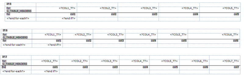
1) В RTF для обозначения элементов мы должны были ставить тег <?ELEMENT_NAME?>, а в XLS мы должны писать в свойствах ячейки, где у нас будет находиться элемент тег XDO_?ELEMENT_NAME?. Пример:
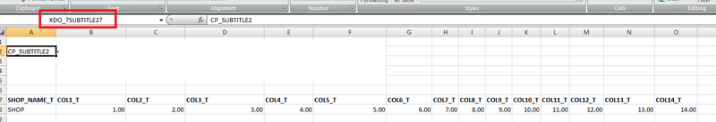
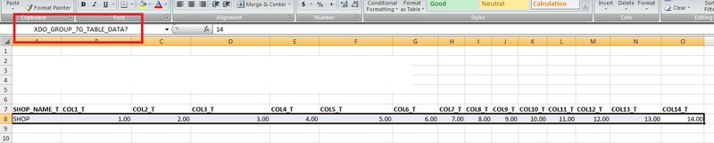
2) В RTF для обозначания открытия групп мы должны были ставить тег <? for-each: GROUP_NAME?> и для закрытия групп должны были ставить тег <?end for-each?> ,a в XLS мы должны выделить ячейки, которые будут заполнены данными из нашей группы и поставить им в качестве свойства XDO_GROUP_?GROUP_NAME?. Это быдет выглядеть так:
3) Будьте внимательными с тем, что пишете в самой клетке, так как вы можете задавать тип данных, которые будут находиться в клетке с помощью обычного Excel функционала, то и то, что написано в клетке должно соответствовать этому типу. Единственное, что у меня не получилось, это получить на выходе дату как даты, пришлось писать для этого небольшой макрос. Ах да, теперь мы можем дополнять наши габлоны макросами, что не было возможно в RTF шаблонах для Excel.
4) Обязательно должна присутствовать отдельная вкладка XDO_METADATA:

Всё, что написано до «Data Constraints:» включая менять не нужно и это должно присутствовать во всех XLS шаблонах. То, что ниже уже ваши функции. Поддерживается XSL, не знаю насчёт остальных. Если элемент находится вне групп, то его нужно получать через xsl:value-of select. Ко всем элементам в этой вкладке нужно обращаться через .//ELEMENT_NAME.
Послесловие
При использовании XLS шаблона мне больше не нужно было создавать для каждого поличества колонок отдельный вариант таблицы. Достаточно сделать таблицу для максимального количества колонок. Колонки, в которых будут присутствовать данные будут заполняться автоматически, в которых данных не будет так и будут оставаться пустыми. Это позволяет избежать лишней работы.
Дополнительную информацию по возможностям создания таких шаблонов можно найти по этой ссылке.
Надеюсь кому-то это поможет избежать лишних хлопот с составление шаблонов.
Содержание
- Xdo excel что это
- Map Data Fields and Groups
- Use Excel Defined Names for Mapping
- Use «XDO_» Prefix to Create Defined Names
- Use Native Excel Functions with the «XDO_» Defined Names
- About the XDO_METADATA Sheet
- Create the XDO_METADATA Sheet
- Format of the XDO_METADATA Sheet
- Hide the XDO_METADATA Sheet
- Enable Excel Template Scalability
- Enable Excel Template Scalability at the Template Level
- Enable Excel Template Scalability at the System Level
- Enable Excel Template Scalability at the Report Level
- Creating Excel Templates
- Introduction
- Features of Excel Templates
- Limitations of Excel Templates
- Prerequisites
- Supported Output
- Desktop Tools
- Sample Excel Templates
- Concepts
- Identifying Data Field Placeholders and Groups
- Use of Excel Defined Names
- About the XDO_ Defined Names
- Using Native Excel Functions
- About the XDO_METADATA Sheet
- Building a Simple Template
- Step 1: Obtain sample XML data from your data model
- Step 2: Open the BlankExcelTemplate.xls file and save as your template name
- Step 3: Design the layout in Excel
- Step 4: Assign the BI Publisher defined names
- Applying a Defined Name to a Cell
- Understanding Groups
- To Create Groups in the Template
- Step 5: Prepare the XDO_METADATA Sheet
- Format of the XDO_METADATA Sheet
- Creating the XDO_METADATA Sheet
- Adding the Calculation for the XDO_?TOTAL_SALARY? Field
- Step 6: Test the template
- Formatting Dates
- Defining BI Publisher Functions
- Reporting Functions
- Splitting the Report into Multiple Sheets
- Declaring and Passing Parameters
- Defining a Link
- Importing and Calling a Subtemplate
- Referencing Java Extension Libraries
- Defining Border and Underline Styles
- Skipping a Row
- Grouping Functions
- Grouping the data
- Regrouping the Data
- Preprocessing the Data Using an XSL Transformation (XSLT) File
- Using the Template Viewer to Debug a Template
Xdo excel что это
Similar to RTF template design, Excel template design follows the paradigm of mapping fields from the XML data to positions in the Excel worksheet.
Excel templates make use of features of Excel in conjunction with special Publisher syntax to achieve this mapping. In addition to direct mapping of data elements, Excel templates support more complex formatting instructions by defining the cell ranges and the commands in a separate worksheet designated to contain these commands. This sheet is called the XDO_METADATA sheet.
Map Data Fields and Groups
Excel templates use named cells and groups of cells to enable Publisher to insert data elements.
Cells are named using Publisher syntax to establish the mapping back to the XML data. The cell names are also used to establish a mapping within the template between the named cell and calculations and formatting instructions defined on the XDO_METADATA sheet.
The template content and layout must correspond to the content and hierarchy of the XML data file used as input to the report. Each group of repeating elements in the template must correspond to a parent-child relationship in the XML file. If the data isn’t structured to match the desired layout in Excel, you can regroup the data using XSLT preprocessing or the grouping functions. However, for the best performance and least complexity it’s recommended that the data model be designed with the report layout in mind.
Use Excel Defined Names for Mapping
Publisher uses the Excel defined names feature to identify data fields and repeating elements.
A defined name in Excel is a name that represents a cell, range of cells, formula, or constant value.
The Template Builder for Excel automatically creates the defined names when you use it to insert fields and repeating groups. You can also insert the defined names manually. The defined names used in the Excel template must use the syntax described in this chapter and follow the Microsoft guidelines described in the Microsoft Excel help document. Note that Publisher defined names are within the scope of the template sheet.
When you create an Excel Template manually (that is, NOT using the Publisher Desktop Excel Template Builder), you must provide default values for all marked up cells XDO_?. The default values must match to the data type of the report data XML file. Without default values for the XDO_? cells, the output cells generated from those template cells may lose formatting and the result is unpredictable. If you use Publisher Desktop to create an Excel Template, the default values are automatically supplied with the first row of sample data in the report data file.
Use «XDO_» Prefix to Create Defined Names
The Publisher defined names are Excel defined names identified by the prefix «XDO_».
Creating the defined name with the Publisher code in the template creates the connection between the position of the code in the template and the XML data elements, and also maintains the ability to dynamically grow data ranges in the output reports, so that these data ranges can be referenced by other formula calculations, charts, and macros.
Use Native Excel Functions with the «XDO_» Defined Names
You can use the XDO_ defined names in Excel native formulas as long as the defined names are used in a simple table.
When a report is generated, Publisher automatically adjusts the region ranges for those named regions so that the formulas calculate correctly.
However, if you create nested groups in the template, then the cells generated in the final report within the grouping can no longer be properly associated to the correct name. In this case, the use of XDO_ defined names with native Excel functions cannot be supported.
About the XDO_METADATA Sheet
Each Excel template requires a sheet within the template workbook called «XDO_METADATA».
Publisher uses this sheet in the template in the following ways:
To identify the template as an Excel template.
To insert the code for the field and group mappings you create with the Template Builder.
As the template designer, you also use this sheet to specify more advanced calculations and processing instructions to perform on fields or groups in the template. Publisher provides a set of functions to provide specific report features. Other formatting and calculations can be expressed in XSLT.
Create the XDO_METADATA Sheet
When you begin the design of a new Excel template using the Template Builder, the first time you use one of the Insert functions the Template Builder automatically creates a hidden XDO_METADATA sheet. A message informs you that the sheet has been created.
Publisher creates the sheet as a hidden sheet. Use the Excel Unhide command to view and edit the XDO_METADATA sheet.
Format of the XDO_METADATA Sheet
The XDO_METADATA sheet is created with the format shown in this figure. The format consists of two sections: the header section and the data constraints section. Both sections are required.
In the header section, all the entries in column A must be listed, but a value is required for only one: Template Type, as shown. The entries in Column A are:
Preprocess XSLT File
Last Modified Date
Last Modified By
The Data Constraints section is used to specify the data field mappings and other processing instructions. Details are provided in the following sections.
Hide the XDO_METADATA Sheet
Oracle recommends that you hide the XDO_METADATA sheet before uploading the completed template to the Publisher catalog to prevent its inclusion in the final report output. Use the Excel Hide command to hide the sheet before uploading the template to the server.
Enable Excel Template Scalability
Enable Excel template scalability to process large data to output reports in Excel format.
If you try to publish reports with large amounts of data as Excel spreadsheets, you might encounter memory issues because the limit of an Excel sheet is 65536 rows. If you enable an Excel template to scale, that template divides a large amount of data into multiple sheets, which helps to avoid memory issues. You can enable Excel template scalability at the system level, the report level, or the Excel template level. The template level setting overrides the report level setting, and the report level setting overrides the system level setting. To ensure backward compatibility, Excel template scalability is set to false by default.
An Excel template that’s enabled to scale does the following to avoid memory issues:
- Flows data into multiple sheets when the data size is more than 65536 rows in a table.
- Flushes memory of every N rows after those N rows are processed for rendering the Excel report.
By default, the flush cell size = 3000 *100 (rows * columns). N = 3000 * 100 / Actual_columns_in_your_ Excel_template_sheet
You can override this flush cell size by specifying the flush cell size (XDO_FLUSH_CELLSIZE_? flush_cell_size ) below the «Data Constraints:» line in the XDO_METADATA sheet in the Excel template. An XDO_GROUP table might not work properly if the final report size of an XDO_GROUP table is greater than the flush cell size.
Enable Excel Template Scalability at the Template Level
You can enable scalability in an Excel template to avoid running out of memory while publishing large amounts of data to an Excel spreadsheet.
- Open the Excel template.
- Select the XDO_METADATA sheet in the Excel template.
- Below the «Data Constraints:» line, enter XDO_SCALABLE_? in Column A, and type true in column B.
Enable Excel Template Scalability at the System Level
As an administrator, you can set a runtime property to enable scalability for all Excel templates.
- As an administrator, navigate to the Runtime Configuration page.
- Scroll down to view the Excel template properties.
- Set the Enable Scalable Mode property to true.
Enable Excel Template Scalability at the Report Level
As a report author, you can set a report level property to enable scalability for the Excel template used by the report.
Источник
Creating Excel Templates
This chapter covers the following topics:
Introduction
An Excel template is a report layout that you design in Microsoft Excel for retrieving and formatting your enterprise reporting data in Excel. Excel templates provide a set of special features for mapping data to worksheets and for performing additional processing to control how your data is output to Excel workbooks.
Features of Excel Templates
With Excel templates you can:
Define the structure for your data in Excel output
Split hierarchical data across multiple sheets and dynamically name the sheets
Create sheets of data that have master-detail relationships
Use native XSL functions in your data to manipulate it prior to rendering
Use native Excel functionality
Limitations of Excel Templates
The following are limitations of Excel templates:
For reports that split the data into multiple sheets, images are not supported. If the template sheet includes images, when the data is split into multiple sheets, the images will show only on the first sheet.
There is no tool to facilitate the markup of the template with BI Publisher tags; all tags must be manually coded. Some features require the use of XSL and XSL Transformation (XSLT) specifications
Prerequisites
Following are prerequisites for designing Excel templates:
Microsoft Excel 2003 or later. The template file must be saved as Excel 97-2003 Workbook binary format (*.xls).
To use some of the advanced features, the report designer will need knowledge of XSL and XSLT.
The report data model has been created.
Supported Output
Excel templates generate Excel binary (.xls) output only.
Desktop Tools
BI Publisher provides a downloadable add-in to Excel that enables you to preview your template with sample data. This facilitates design by enabling you to test and edit your template without having to upload it to the BI Publisher catalog first.
The Template Builder for Excel is installed automatically when you install the Template Builder for Word. The tools can be downloaded from the Home page of Oracle Business Intelligence Publisher or Oracle Business Intelligence Enterprise Edition, as follows:
Under the Get Started region, click Download BI Publisher Tools .
Sample Excel Templates
The Template Builder includes sample Excel templates.
To access the samples from a Windows desktop:
Click Start , then Programs , then Oracle BI Publisher Desktop , then Samples , then Excel .
This will launch the folder that contains the Excel sample templates.
Concepts
Similar to RTF template design, Excel template design follows the paradigm of mapping fields from your XML data to positions in the Excel worksheet. Excel templates make use of features of Excel in conjunction with special BI Publisher syntax to achieve this mapping. In addition to direct mapping of data elements, Excel templates also utilize a special sheet (the XDO_METADATA sheet) to specify and map more complex formatting instructions.
Identifying Data Field Placeholders and Groups
Excel templates use named cells and groups of cells to enable BI Publisher to insert data elements. Cells are named using BI Publisher syntax to establish the mapping back to the XML data. The cell names are also used to establish a mapping within the template between the named cell and calculations and formatting instructions that are defined on the XDO_METADATA sheet.
Your template content and layout must correspond to the content and hierarchy of the XML data file used as input to your report. Each group of repeating elements in your template must correspond to a parent-child relationship in the XML file. If your data is not structured to match the desired layout in Excel it is possible to regroup the data using XSLT preprocessing or the grouping functions. However, for the best performance and least complexity it is recommended that the data model be designed with the report layout in mind.
Use of Excel Defined Names
The Excel defined names feature is used to identify data fields and repeating elements. A defined name in Excel is a name that represents a cell, range of cells, formula, or constant value.
Tip: To learn more about defined names and their usage in Microsoft Excel 2007, see the Microsoft help topic: «Define and use names in formulas.»
The defined names used in your Excel template must use the syntax described in this chapter, as well as follow the Microsoft guidelines described in the Microsoft Excel help document. Note that BI Publisher defined names are within the scope of the template sheet.
About the XDO_ Defined Names
The BI Publisher defined names are Excel defined names identified by the prefix «XDO_». Marking up the placeholders in the template files creates the connection between the position of the placeholders in the template and the XML data elements, and also maintains the ability to dynamically grow data ranges in the output reports, so that these data ranges can be referenced by other formula calculations, charts, and macros.
Using Native Excel Functions
You can use the XDO_ defined names in Excel native formulas as long as the defined names are used in a simple table. When a report is generated, BI Publisher will automatically adjust the region ranges for those named regions so that the formulas calculate correctly.
However, if you create nested groups in your template, the cells generated in the final report within the grouping can no longer be properly associated to the correct name. In this case, the use of XDO_ defined names with native Excel functions cannot be supported.
About the XDO_METADATA Sheet
Each Excel template requires a sheet within the template workbook called «XDO_METADATA». Use this sheet to identify your template to BI Publisher as an Excel template. This sheet is also used to specify calculations and processing instructions to perform on fields or groups in the template. BI Publisher provides a set of functions to provide specific report features. Other formatting and calculations can be expressed in XSLT.
It is recommended that you hide the XDO_METADATA sheet before you upload your completed template to the BI Publisher catalog. This will prevent report consumers from seeing it in the final report output.
Building a Simple Template
This section will demonstrate the concepts of Excel templates by walking through the steps to create a simple Excel template and testing it with the Excel Template Builder. This procedure will follow these steps:
Obtain sample XML data from your data model.
Open the BlankExcelTemplate.xls file and save as your template name.
Design the layout in Excel.
Assign the BI Publisher defined names.
Prepare the XDO_METADATA sheet.
Test the template using the desktop Excel Template Builder.
Step 1: Obtain sample XML data from your data model
You need sample data in order to know your field names and the hierarchical relationships to properly mark up the template. For information on saving sample data from your report data model, see the topic «Testing Data Models and Generating Sample Data» in the Oracle Fusion Middleware Data Modeling Guide for Oracle Business Intelligence Publisher .
If you do not have access to the report data model, but you can access the report, you can alternatively save sample data from the report viewer. To save data from the report viewer:
In the BI Publisher catalog, navigate to the report.
Click Open to run the report in the report viewer.
Click the Actions menu, then click Export , then click Data . You will be prompted to save the XML file.
Save the file to a local directory.
The sample data for this example is a list of employees by department. Note that employees are grouped and listed under the department.
Step 2: Open the BlankExcelTemplate.xls file and save as your template name
Note: It is recommended that you install the Template Builder for Excel. For information on downloading the tool, see Desktop Tools.
The Template Builder installation includes a set of sample Excel templates, including a sample blank Excel template called BlankExcelTemplate.xls. This template file contains a blank Sheet1 and the XDO_METADATA sheet. It is recommended that you either start with this provided template or copy the XDO_METADATA sheet into your own Excel workbook.
Tip: If you are building a new template from an existing template, be sure to clear any existing defined names in the template sheet.
To open the BlankExcelTemplate.xls:
From a Windows desktop, click Start , then Programs , then Oracle BI Publisher Desktop , then Samples , then Excel .
In the Excel Templates sample folder, double-click BlankExcelTemplate.xls to open it.
Save the file as your selected name in the Microsoft Excel 97-2003 Workbook format (*.xls).
Step 3: Design the layout in Excel
In Excel, determine how you want to render the data and create a sample design, as shown in the following figure:
The design shows a department name and a row for each employee within the department. You can apply Excel formatting to the design, such as font style, shading, and alignment. Note that this layout includes a total field. The value for this field is not available in the data and will require a calculation.
Step 4: Assign the BI Publisher defined names
To code this design as a template, mark up the cells with the XDO_ defined names to map them to data elements. The cells must be named according to the following format:
Data elements: XDO_? element_name ?
XDO_ is the required prefix and
? element_name ? is either:
the XML tag name from your data delimited by «?»
a unique name that you will use to map a derived value to the cell
For example: XDO_?EMPLOYEE_ID?
Data groups: XDO_GROUP_? group_name ?
XDO_GROUP_ is the required prefix and
? group_name ? is the XML tag name for the parent element in your XML data delimited by «?».
a unique name that you will use to define a derived grouping logic
For example: XDO_GROUP_?DEPT?
Note that the question mark delimiter, the group_name , and the element_name are case sensitive.
Applying a Defined Name to a Cell
Click the cell in the Excel worksheet.
Click the Name box at the left end of the formula bar. The default name will display in the Name box. By default, all cells are named according to position, for example: A8.
In the Name box, enter the name using the XDO_ prefix and the tag name from your data. For example: XDO_?EMP_NAME?
The following figure shows the defined name for the Employee Name field entered in the Name box:
Repeat for each of the following data fields: DEPARTMENT_NAME, EMPLOYEE_ID, EMAIL, PHONE_NUMBER, and SALARY.
Tip: If you navigate out of the Name box without pressing Enter, the name you entered will not be maintained.
You cannot edit the Name box while you are editing the cell contents.
The name cannot be more than 255 characters in length.
For the total salary field, a calculation will be mapped to that cell. For now, name that cell XDO_?TOTAL_SALARY?. The calculation will be added later.
After you have entered all the fields, you can review the names and make any corrections or edits using the Name Manager feature of Excel. Access the Name Manager from the Formulas tab in Excel as shown:
After you have named all the cells for this example, the Name Manager dialog will appear as shown:
You can review all your entries and update any errors through this dialog.
Understanding Groups
A group is a set of data that repeats for each occurrence of a particular element. In the sample template design, there are two groups:
For each occurrence of the element, , the employee’s data (name, e-mail, telephone, salary) will display in the worksheet.
For each occurrence of the element, the department name and the list of employees belonging to that department will display.
In other words, the employees are «grouped» by department and each employee’s data is «grouped» by the employee element. To achieve this in the final report, add grouping tags around the cells that are to repeat for each grouping element.
Note that your data must be structured according to the groups you want to create in your template. The structure of the data for this example
establishes the grouping desired for the report.
To Create Groups in the Template
Highlight the cells that make up the group. In this example the cells are A8 — E8.
Click the Name box at the left end of the formula bar and enter the name using the XDO_GROUP_ prefix and the tag name for the group from your data. For example: XDO_GROUP_?EMPS?
The following figure shows the XDO_GROUP_ defined named entered for the Employees group. Note that just the row of employee data is highlighted. Do not highlight the headers. Note also that the total cell XDO_?TOTAL_SALARY? is not highlighted.
To define the department group, include the department name cell and all the employee fields beneath it (A5-E9) as shown in the following figure:
Enter the name for this group as: XDO_GROUP_?DEPT? to match the group in the data. Note that the XDO_?TOTAL_SALARY? cell is included in the department group to ensure it repeats at the department level.
Step 5: Prepare the XDO_METADATA Sheet
BI Publisher requires the presence of a sheet called «XDO_METADATA» to process the template. This sheet must follow the specifications defined here.
Format of the XDO_METADATA Sheet
The XDO_METADATA sheet must have the format shown in the following figure:
The format consists of two sections: the header section and the data constraints section. Both sections are required. In the header section, all the entries in column A must be listed, but a value is required for only one: Template Type, as shown. The Data Constraints section does not require any content, but also must be present as shown.
This procedure describes how to set up the sheet for this sample Excel template to run. For the detailed description of the functionality provided by the XDO_METADATA sheet see Defining BI Publisher Functions.
Creating the XDO_METADATA Sheet
If you copied the XDO_METADATA sheet in Step 2, skip this section and proceed to Adding the Calculation for the XDO_?TOTAL_SALARY? Field; otherwise, set up the hidden sheet as follows:
Create a new sheet in your Excel Workbook and name it «XDO_METADATA».
Create the header section by entering the following variable names in column A, one per row, starting with row 1:
Preprocess XSLT File
Last Modified Date
Last Modified By
Skip a row and enter «Data Constraints» in column A of row 10.
In the header region, for the variable «Template Type» enter the value: TYPE_EXCEL_TEMPLATE
Adding the Calculation for the XDO_?TOTAL_SALARY? Field
Earlier in this procedure you assigned the defined named XDO_?TOTAL_SALARY? to the cell that is to display the total salaries listed in the SALARY column. In this step, you will add the calculation to the Data Constraints section of the XDO_METADATA sheet and map the calculation to the XDO_?TOTAL_SALARY? field.
In the Data Constraints section, in Column A, enter the defined name of the cell: XDO_?TOTAL_SALARY?
In Column B enter the calculation as an XPATH function. To calculate the sum of the SALARY element for all employees in the group, enter the following:
The completed XDO_METADATA sheet is shown in the following figure:
Step 6: Test the template
If you have installed the Template Builder for Excel, the BI Publisher tab will appear on the ribbon menu as shown in the following figure:
To preview your report using sample data:
Click Sample XML . You will be prompted to select the sample data file.
The sample data will be applied to your template and the output document will be opened in a new workbook. The following figure shows the preview of the template with the sample data:
Formatting Dates
Excel cannot recognize canonical date format. If the date format in your XML data is in canonical format, that is, YYYY-MM-DDThh:mm:ss+HH:MM, you must apply a function to display it properly.
One option to display your date is to use the Excel REPLACE and SUBSTITUTE functions. This option will retain the full date and timestamp. If you only require the date portion in your data (YYY-MM-DD), another option is to use the DATEVALUE function. The following example shows how to use both options.
Example: Formatting a Canonical Date in Excel
Using the Employee by Department template and data from the first example, assume you want to add the HIRE_DATE element to the layout to and display the date as shown in Column E of the following figure:
To format the date as shown above, follow these steps:
Copy and paste a sample value for HIRE_DATE from the XML data into the cell that is to display the HIRE_DATE field. For example:
into the E8 cell.
Assign the cell the defined name XDO_?HIRE_DATE? to map it to the HIRE_DATE element in the data, as shown in the following figure:
If you do nothing else, the HIRE_DATE value will display as shown. To format the date as «3-Feb-96», you must apply a function to that field and display the results in a new field.
Insert a new Hire Date column. This will now be column F as shown in the following figure:
In the new Hire Date cell (F8), enter one of the following Excel functions:
To retain the full date and timestamp, enter:
To retain only the date portion (YYY-MM-DD), enter:
After you enter the function, it will populate the F8 cell as shown in the following figure:
Apply formatting to the cell.
Right-click the F8 cell. From the menu, select Format Cells. In the Format Cells dialog, select Date and the desired format, as shown in the following figure:
The sample data in the F8 cell now displays as 3-Feb-96.
Finally, hide the E column, so that report consumers will not see the canonical date that is converted.
Defining BI Publisher Functions
BI Publisher provides a set of functions to achieve additional reporting functionality. You define these functions in the Data Constraints region of the XDO_METADATA sheet.
The functions make use of Columns A, B, and C in the XDO_METADATA sheet as follows:
Use Column A to declare the function or to specify the defined name of the object to which to map the results of a calculation or XSL evaluation.
Use Column B to enter the special XDO-XSL syntax to describe how to control the data constraints for the XDO function, or the XSL syntax that describes the special constraint to apply to the XDO_ named elements.
Use Column C to specify additional instructions for a few functions.
The functions are described in the following three sections:
Reporting Functions
The following functions can be added to your template using the commands shown and a combination of BI Publisher syntax and XSL. A summary list of the commands is shown in the following table. See the corresponding section for details on usage.
| Function | Commands |
|---|---|
| Split the report data into multiple sheets | XDO_SHEET_? with XDO_SHEET_NAME_? |
| Define a parameter | XDO_PARAM_? n ? |
| Define a link | XDO_LINK_? link object name ? |
| Import a subtemplate | XDO_SUBTEMPLATE_? n ? |
| Reference Java extension libraries | XDO_EXT_? n ? |
Splitting the Report into Multiple Sheets
Note: Images are not supported across multiple sheets. If the template sheet includes images, when the data is split into multiple sheets, the images will show only on the first sheet.
Use the this set of commands to define the logic to split the report data into multiple sheets:
Use XDO_SHEET_? to define the logic by which to split the data onto a new sheet.
Use XDO_SHEET_NAME_? to specify the naming convention for each sheet.
| Column A Entry | Column B Entry | Column C Entry |
|---|---|---|
| XDO_SHEET_? | xsl_evaluation to split the data ?> Example: |
n/a |
| XDO_SHEET_NAME_? | xsl_expression to name the sheet ?> Example: |
(Optional) original sheet name ?> Example: |
XDO_SHEET_? must refer to an existing high-level node in your XML data. The example will create a new sheet for each occurrence of in the data.
If your data is flat you cannot use this command unless you first preprocess the data to create the desired hierarchy. To preprocess the data, define the transformation in an XSLT file, then specify this file in the Preprocess XSLT File field of the header section of the XDO _METADATA sheet. For more information, see Preprocessing the Data Using an XSL Transformation (XSLT) File.
Use XDO_SHEET_NAME_? to define the name to apply to the sheets. In Column B enter the XSL expression to derive the new sheet name. The expression can reference a value for an element or attribute in the XML data, or you can use the string operation on those elements to define your final sheet name. This example:
will name each sheet using the value of DEPARTMENT_NAME concatenated with «-» and the count of employees in the DEPT group.
The original sheet name entry in Column C tells BI Publisher on which sheet to begin the specified sheet naming. If this parameter is not entered, BI Publisher will apply the naming to the first sheet in the workbook that contains XDO_ names. You would need to enter this parameter if, for example, you have a report that contains summary data in the first two worksheets and the burst data should begin on Sheet3. In this case, you would enter in Column C.
Example: Splitting the data into multiple sheets
Using the employee data shown in the previous example. This example will:
Create a new worksheet for each department
Name each worksheet the name of the department with the number of employees in the department, for example: Sales-21.
Enter the defined names for each cell of employee data and create the group for the repeating employee data:
Note: Do not create the grouping around the department because the data will be split by department.
Enter the following in the Data Constraints section of the XDO_METADATA sheet:
The entries are shown in the following figure:
The following figure shows the generated report. Each department data now displays on its own sheet, which shows the naming convention specified:
Declaring and Passing Parameters
To define a parameter, use the XDO_PARAM_? n ? function to declare the parameter, then use the $ parameter_name syntax to pass a value to the parameter. A parameter must be defined in your data model.
To declare the parameter, use the following command:
| Column A Entry | Column B Entry |
|---|---|
| XDO_PARAM_? n ? where n is unique identifier for the parameter |
parameter_name ; parameter_value ?> where parameter_name is the name of the parameter from the data model and parameter_value is the optional default value. For example: |
To use the value of the parameter directly in a cell, refer to the parameter as $ parameter_name in the definition for the XDO_ defined name, as follows:
| Column A Entry | Column B Entry |
|---|---|
| XDO_PARAM_?parameter_name? for example: XDO_PARAM_?Country? |
parameter_name ?>. For example: |
You can also refer to the parameter in other logic or calculations in the XDO_METADATA sheet using $parameter_name.
Example: Defining and passing a parameter
In this example, declare and reference a parameter named Country.
In the template sheet, mark the cell with a defined name. In the figure below, the cell has been marked with the defined name XDO_?Country?
In the hidden sheet assign that cell the parameter value as follows:
Defining a Link
Use the XDO_LINK_? command to define a hyperlink for any data cell.
| Column A Entry | Column B Entry |
|---|---|
| XDO_LINK_? cell object name ? For example: XDO_LINK_?INVOICE_NO? |
xsl statement to build the dynamic URL > For example: |
Example: Defining a Link
Assume your company generates customer invoices. The invoices are stored in a central location accessible by a Web server and can be identified by the invoice number (INVOICE_NO). You can generate a report that creates a dynamic link to each invoice as follows:
In your template sheet, assign the cell that is to display the INVOICE_NO the XDO defined name: XDO_?INVOICE_NO?.
In the XDO_METADATA sheet, enter the following:
The entries in Excel are shown in the following figure:
The report output will display as shown in the following figure. The logic defined in the XDO_METADATA sheet will be applied to create a hyperlink for each INVOICE_NO entry:
Importing and Calling a Subtemplate
Use these commands to declare XSL subtemplates that you can then call and reference in any of the XDO_ commands.
Note: The Template Builder for Excel does not support preview for templates that import subtemplates.
To import the subtemplate, enter the following command:
| Column A Entry | Column B Entry |
|---|---|
| XDO_SUBTEMPLATE_? n ? where n is a unique identifier. For example: XDO_SUBTEMPLATE_?1? . |
path to subtemplate.xsb ?»/> For example: |
To call the subtemplate, declare the cell name for which the results should be returned in Column A, then enter the call-template syntax with any other XSL processing to be performed:
| Column A Entry | Column B Entry |
|---|---|
| XDO_? cell object name ? | template_name «> |
For more information on XSL subtemplates and creating the subtemplate object in the catalog, see Designing XSL Subtemplates.
Example: Importing and Calling a Subtemplate
Assume you have the following subtemplate uploaded to the BI Publisher catalog as PaymentsSummary-SubTemplate.xsb. This subtemplate will evaluate the value of a parameter named pPayType and based on the value, return a string that indicates the payment type:
In your Excel template, you have defined a field with the XDO Defined Name XDO_?TYPE?, which will be populated based on the string returned from code performed in the subtemplate, as shown in the following figure:
Enter the following in the Data Constraints region:
| Column A Entry | Column B Entry |
|---|---|
| XDO_SUBTEMPLATE_?1? | |
| XDO_?TYPE? |
The XDO_SUBTEMPLATE_?1? function imports the subtemplate from the BI Publisher catalog.
The XDO_?TYPE? cell entry maps the results of the subtemplate processing entered in Column B.
Referencing Java Extension Libraries
You can include the reference to a Java extension library in your template and then call methods from this library to perform processing in your template. Use this command to reference the Java extension libraries:
| Column A Entry | Column B Entry |
|---|---|
| XDO_EXT_? n ? where n is a unique identifier. Example: XDO_EXT?1? |
exension library «?> Example: |
You can have multiple extension libraries defined in a single template file.
Example: Calling a Java Extension Library
Assume the extension library includes the following two methods that you want to call in your template:
After you have declared the library as shown above, specify the cell to which you want to apply the method by entering the XDO defined name in Column A and calling the function in Column B. For example:
The following commands require that specific formatting attributes be present in the XML data file. A summary list of the commands is shown in the following table. See the corresponding section for details on usage.
| Function | Command |
|---|---|
| Define border and underline styles | XDO_STYLE_ n _? cell object name ? |
| Skip a row | XDO_SKIPROW_? cell object name ? |
Defining Border and Underline Styles
While you can define a consistent style in the template using Excel formatting, the XDO_STYLE command enables you to define a different style for any data cell dynamically based on the XML data.
With the XDO_STYLE command you specify the cell to which to apply the style, the logic to determine when to apply the style, and the style type to apply. The style value must be present in the XML data.
| Column A Entry | Column B Entry | Column C Entry |
|---|---|---|
| XDO_STYLE_n_? cell_object_name ? For example: XDO_STYLE_1_?TOTAL_SALARY? |
xsl evaluation that returns a supported value > For example: |
Style type For example: BottomBorderStyle |
BI Publisher supports the following normal Excel style types and values:
| Style Type | Supported Values (Must be in returned by evaluation in Column B) |
Supported Types (Enter in Column C) |
|---|---|---|
| Normal | BORDER_NONE BORDER_THIN BORDER_MEDIUM BORDER_DASHED BORDER_DOTTED BORDER_THICK BORDER_DOUBLE BORDER_HAIR BORDER_MEDIUM_DASHED BORDER_DASH_DOT BORDER_MEDIUM_DASH_DOT BORDER_DASH_DOT_DOT BORDER_MEDIUM_DASH_DOT_DOT BORDER_SLANTED_DASH_DOT |
BottomBorderStyle TopBorderStyle LeftBorderStyle RightBorderStyle DiagonalLineStyle |
You can also set a color using one of the following types:
| Style Type | Supported Value (Must be in returned by evaluation in Column B) |
Supported Types (Enter in Column C) |
|---|---|---|
| Normal | When you set Color Style, give the value in RRBBGG hex format, for example: borderColor=»0000FF» | BottomBorderColor TopBorderColor LeftBorderColor RightBorderColor DiagonalLineColor |
BI Publisher also supports the underline type with the following values:
| Style Type | Supported Values (Must be in returned by evaluation in Column B) |
Supported Type (Enter in Column C) |
|---|---|---|
| Underline | UNDERLINE_NONE UNDERLINE_SINGLE UNDERLINE_DOUBLE UNDERLINE_SINGLE_ACCOUNTING UNDERLINE_DOUBLE_ACCOUNTING |
UnderlineStyle |
You can have multiple underline styles defined for a single cell.
Example: Defining Styles
To apply a style in a template, the style value must be present in the data. In this example, a border style and an underline style will be applied to the DEPT_TOTAL_SALARY field shown in the Excel template.
For this example, the following data is used. Note that the DEPT_TOTAL_SALARY element in the data has these attributes defined:
The value of each of these attributes will be used to apply the defined style based on logic defined in the template.
In the Excel template assign the defined named XDO_?DEPT_TOTAL_SALARY? to the field that is to display the DEPT_TOTAL_SALARY from the data.
In the XDO_METADATA sheet, enter the following:
To define the top border style, enter:
| Column A Entry | Column B Entry | Column C Entry |
|---|---|---|
| XDO_STYLE_1_?DEPT_TOTAL_SALARY? | TopBorderStyle |
The entry in Column A maps this style command to the cell assigned the name XDO_?DEPT_TOTAL_SALARY?
The entry in Column B retrieves the style value from the attribute borderStyle of the DEPT_TOTAL_SALARY element. Note from the sample data that the value for borderStyle is «BORDER_DOUBLE».
The entry in Column C tells BI Publisher to apply a TopBorderStyle to the cell.
To define the top border color, enter:
| Column A Entry | Column B Entry | Column C Entry |
|---|---|---|
| XDO_STYLE_2_?DEPT_TOTAL_SALARY? | TopBorderColor |
The entry in Column A maps this style command to the cell assigned the name XDO_?DEPT_TOTAL_SALARY?
The entry in Column B retrieves the style value from the attribute borderColor of the DEPT_TOTAL_SALARY element. Note from the sample data that the value for borderColor is «0000FF» (blue).
The entry in Column C tells BI Publisher to apply a TopBorderColor to the cell.
To define the underline style, enter:
| Column A Entry | Column B Entry | Column C Entry |
|---|---|---|
| XDO_STYLE_3_?DEPT_TOTAL_SALARY? | UnderlineStyle |
The entry in Column A maps this style command to the cell assigned the name XDO_?DEPT_TOTAL_SALARY?
The entry in Column B retrieves the style value from the attribute underLineStyle of the DEPT_TOTAL_SALARY element. Note from the sample data that the value for underLineStyle is «UNDERLINE_DOUBLE_ACCOUNTING».
The entry in Column C tells BI Publisher to apply the UnderLineStyle to the cell.
The following figure shows the three entries in the Data Constraints region:
When you run the report, the style commands will be applied to the XDO_?DEPT_TOTAL_SALARY? cell, as shown in the following figure:
Skipping a Row
Use the XDO_SKIPROW command to suppress the display of a row of data in a table when the results of an evaluation defined in Column B return the case insensitive string «True».
| Column A Entry | Column B Entry |
|---|---|
| XDO_SKIPROW_? cell_object_name ? For example: XDO_SKIPROW_?EMPLOYEE_ID? |
xsl evaluation that returns the string «True»/> For example: |
Example: Skipping a Row Based on Data Element Attribute
In this example, the Excel template will suppress the display of the row of employee data when the EMPLOYEE_ID element includes a «MANAGER» attribute with the value «True».
Assume data as shown below. Note that the EMPLOYEE_ID element for employee Michael Hartstein has the MANAGER attribute with the value «True». The other EMPLOYEE_ID elements in this set do not have the attribute.
To suppress the display of the row of the employee data when the MANAGER attribute is set to «True», enter the following in the Data Constraints section:
| Column A Entry | Column B Entry |
|---|---|
| XDO_SKIPROW_?EMPLOYEE_ID? |
The output from this template is shown in the following figure. Note that the employee Michael Hartstein is not included in the report:
Grouping Functions
Use these functions to create groupings of data in the template.
| Function | Command |
|---|---|
| Group data | XDO_GROUP_? group elemen t? |
| Regroup data | XDO_REGROUP_? |
Grouping the data
Use the XDO_GROUP command to group flat data when your layout requires a specific data grouping, for example, to split the data across multiple sheets.
| Column A Entry | Column B Entry | Column C Entry |
|---|---|---|
| XDO_GROUP_? group element ? For example: XDO_GROUP_?STATE_GROUP? |
xsl beginning groupng logic/> For example: |
xsl ending groupng tags/> For example: |
Define the XSL statements to be placed at the beginning and ending of the section of the group definition marked up by XDO_? cell object name ?. You can mark multiple groups nested in the template, giving each the definition appropriate to the corresponding group.
Regrouping the Data
The XDO_REGROUP regroups the data by declaring the structure using the defined names. It does not require the XSLT logic.
UniqueGroupID is the ID of the group. It can be the same as the levelName or you can assign it unique name.
levelName is the XML level tag name in the XML data file or current-group() in the context of the XDO_ grouping structure.
groupByName is the field name that you want to use for the GroupBy operation for the current group. This name can be empty if the XDO_REGROUP_? command is used for the most inner group.
sortByName is the field name that you want to sort the group by. You can have multiple sortBy fields. If no sortByName is declared, the data from the XML file will not be sorted.
The following shows an example of how to create three nested groupings:
| Column A Entry | Column B Entry |
|---|---|
| XDO_REGROUP_? | XDO_REGROUP_?PAYMENTSUMMARY_Q1?PAYMENTSUMMARY_Q1?PAY_TYPE_NAME? |
In the above definition, the most outer group is defined as PAYMENTSUMMARY_Q1, and it is grouped by PAY_TYPE_NAME
| Column A Entry | Column B Entry |
|---|---|
| XDO_REGROUP_? | XDO_REGROUP_?COUNTRYGRP?XDO_CURRGRP_?COUNTRY? |
The above definition creates a second outer group. The group is assigned the name COUNTRY_GRP and it is grouped by the element COUNTRY.
| Column A Entry | Column B Entry |
|---|---|
| XDO_REGROUP_? | XDO_REGROUP_?STATEGRP?XDO_CURRGRP_?STATE? |
This definition creates the inner group STATEGRP and it includes a sortByName parameter: STATE.
Preprocessing the Data Using an XSL Transformation (XSLT) File
For the best performance, you should design your data model to perform as much of the data processing as possible. When it is not possible to get the required output from data engine, you can preprocess the data using an XSLT file that contains the instructions to transform the data. Some sample use cases may be:
To create groups to establish the necessary hierarchy to support the desired layout
To add style attributes to data elements
To perform complex data processing logic that may be impossible in the Excel Template or undesirable for performance reasons
Note: The Template Builder for Excel does not support preview for templates that require XSLT preprocessing.
To use an XSLT preprocess file:
Create the file and save as .xsl.
Upload the file to the report definition in the BI Publisher catalog, as you would a template:
Navigate to the report in the catalog.
Click Add New Layout .
Complete the fields in the Upload dialog and select «XSL Stylesheet (HTML/XML/Text)» as the template Type .
After upload, click View a List . Deselect Active , so that users will not see this template as an option when they view the report.
Note: For testing purposes, you may want to maintain the XSL template as active to enable you to view the intermediate data when the template is applied to the data. After testing is complete, set the template to inactive.
Save the report definition.
In your Excel template, on the XDO_METADATA sheet, in the Header section, enter the file name for the Preprocess XSLT File parameter. For example: SplitByBrand.xsl
Using the Template Viewer to Debug a Template
If your template preview is not generating the results expected, you can use the Template Viewer to enable trace settings to view debug messages. The Template Viewer also enables you to save and view the intermediate XSL file that is generated after the sample data and template are merged in the XSL-FO processor. If you are familiar with XSL this can be a very useful debugging tool.
The Template Viewer is installed when you install the Template Builder for Word; see Desktop Tools for more information.
To preview with the Template Viewer and view log messages:
Open the Template Viewer:
From your Windows desktop, click Start , then Programs , then Oracle BI Publisher Desktop , then Template Viewer .
Click Browse to locate the folder that contains your sample data file and template file. The data file and template file must reside in the same folder.
Select Excel Templates . The Data and Template regions will display all .xml files and all .xls files present in the directory.

Click the appropriate data and template files to select them.
Select the log level.
From the Output Format list, select Excel.
Click Start Processing .
The Template Viewer will merge the selected data with the selected template and spawn the appropriate viewer. View any log messages in the message box as shown in the following figure:
To view the generated XSL:
In the Template Viewer, select the data and template files and choose Excel output.
On the Tools menu, select Generate XSL file from and then choose Excel Template .
At the prompt, save the generated XSL file.
Navigate to the saved location and open the XSL file in an appropriate viewer.
Источник
Нам нужен Excel!!!
Я постоянно слышу это от пользователей Oracle BI.
Уверен, вы — тоже.
И нам приходилось использовать существующие решения в BI Publisher для предоставления нашим пользователям Excel-отчетов:
Чаще всего использование RTF-шаблонов с выводом в Эксель. Со всеми сопутствующими багами. Ведь такой метод использует обходной маневр – способность Экселя открывать mht-файлы.


Наверняка, вы сталкивались с минусами такого подхода: невозможность точного форматирования выходной разметки, невозможность задания формата ячейки, невозможность разбиения отчета на листы, невозможность использования макросов, вывода графиков и диаграмм. Список можно продолжать.
Частично выручал метод создания отчетов с помощью XSL-шаблонов разметки, но и там большинство «нельзя» оставалось, плюс мы должны были регламентами использования ограничивать браузер (только IE), версию MS Office (2003 и выше), чтобы полученный отчет прозрачно для пользователя открывался в Экселе.
Теперь об этом можно забыть (шучу!).
Уже длительное время команда Oracle, занимающаяся ядром BIPublisher, готовит новый тип шаблонов разметки – XLS.
Прочитать об этом можно на блоге Тима Декстера
В чем-то данная статься является вольным переводом сообщения Тима, в чем-то – дополнением.
Итак, для использования XLS-шаблонов вам в первую очередь потребуется обновить BIPublisher. Для этого скачайте с металинка патч 9546699
Возьмите отформатированный в Экселе шаблон вашего отчета.
Я покажу пример на основе отчета «Balance Letter» из стандартной поставки BIPublisher.
Создайте в нем новый лист с именем XDO_METADATA, на котором поместите общую информацию о шаблоне.
(Не забудьте скрыть затем этот лист.)
На главном листе шаблона выделите область, содержащую повторяющиеся данные по группе G_CURRENCY. В поле именованных диапазонов задайте имя области – XDO_GROUP_?G_CURRENCY?.
G_CURRENCY – это элемент XML-файла, представляющий основную группировку выводимых данных.
Выделите группу низшего уровня. Аналогично, задайте ей имя – XDO_GROUP_?G_INVOICES?

Теперь для каждой ячейки низшей группы задайте имя, соответствующее элементу XML-файла данных.

Если вы где-то ошиблись в имени, либо хотите увидеть все ваши mapping’и:


На данном этапе будем считать наш шаблон разметки завершенным.
Выделенные области пока оставим без изменения.

Загрузим созданный шаблон разметки через интерфейс BIPublisher (к сожалению, пока нет возможности проверять шаблоны локально, как это сделано для RTF-шаблонов – через Desktop Template Builder).

Запустим отчет на выполнение. Полученный файл является «чистым» Эксель-файлом со всеми вытекающими последствиями.

Теперь попробуем понять — как это все работает.
Откроем системную временную папку – у меня это «C:WindowsTEMP».
После запуска отчета с Эксель-шаблоном появятся 2 новых файла:

Первый файл – это XSL, полученный из подготовленного Excel-файла. Именно в нем содержатся все определенные нами группировки.
Второй файл – XML с данными, полученный XSLT-трансформацией XML-файла данных и XSL-файла с предыдущей картинки.
Видим, что остались видны все имена именованных диапазонов исходного шаблона разметки. Именно по ним в итоге полученный XML-файл преобразуется в Excel.
Итак, раз ничего сверхъестественного в данном механизме нет – можно попробовать использовать привычные XSL-конструкции.
Попробуем реализовать вывод информации, которая получается конкатенацией статического текста и динамических данных.
(Если делать это через механизм mapping’а, то придется мудрить с разбиением/схлапыванием ячеек).
На скрытом листе XDO_METADATA определим новую переменную, значение которой получается конкатенацией статического текста и динамического значения кода валюты и суммы по ней.
Присвоим первой ячейке в строке имя, равное определенной нами переменной.

P.S. Официальной документации по данной технологии еще нет. Но уже сейчас понятно, что возможности по созданию Excel-отчетов – замечательные.
Раз есть возможность использования макросов, то можно создавать графики.
Есть возможность динамического разбиения данных по листам Эксель-файла (используя bursting).
Есть возможность вывода данных в таблицах среза.
В следующих статьях я постараюсь раскрыть эти возможности.
P.P.S. Ссылка на архив с примером.
![]()
Summary
Starting with the release of PeopleTools 8.58, PeopleTools can now use Excel Spreadsheets as BI Publisher templates. Before this release, if we wanted to create a spreadsheet using BI Publisher, the fastest way was to use an RTF template with a table and force the output to Excel through the report definition. However, this is more of a “Work Around” than a solution and left a few concepts to be desired.
Now using the Excel templates, we can work directly in Excel to define the report which provides many of the features and tools that the users are requesting.
This document will introduce the basics of using Excel Templates with BI Publisher.
What and Why Excel Templates
Excel templates allow us to generate Excel spreadsheets in BI Publisher using Excel.
Excel templates are not new to BI Publisher. They are just new to PeopleTools’ implementation of BI Publisher. Luckily, there is plentiful documentation, demonstrations, and examples of Excel Templates available. We just need leverage these within our PeopleTools environment.
Just like we used MS Word to create RTF templates, we use Excel to create XLS templates with the same desktop helper (Template Builder).
Now we can create multiple page spreadsheets natively formatted in Excel and delivered through the PeopleTools framework where and when they are needed.
This is a link to the Oracle Excel Template Documentation: docs.oracle.com/html/E22254_03/create_excel_tmpl.htm
BI Publisher Excel Template Basics
Installing the Template Builder
Download the latest version of BI Publisher Desktop Template Builder as per your version of PeopleTools. The easiest way is through your PeopleSoft Application
Home > Reporting Tools > BI Publisher > Setup > Design Helper
Make sure you install the correct 32/64-bit version as per your version of MS Office. Installing the wrong version will create problems. If this does happen, completely uninstall before re-installing the correct version.
If you installed the Desktop helper for MS Word, then you have already installed the Desktop Helper for Excel. Just look for the BI Publisher heading on your ribbon in Excel just an in Word.

Notes on the Excel Template Builder
XLS, Not XLSX
BI Publisher uses the .xls spreadsheets (1997-2003 Workbook), not the modern .xlsx spreadsheets. When coding spreadsheets, you can only use capabilities and functions available to this version. Advanced formatting and functions from the current version will not work.
Hidden XDO_METADATA Sheet
The Template Builder will create a hidden sheet to the Excel workbook when the first field is added. BI Publisher uses this hidden sheet for mapping between the data and the spreadsheet. You might have to edit some of these references and formulas.
To unhide the sheet
- Right click on the worksheet tab
- Select UnHide
- Select XDO_MEDATA


The top section (rows 1-8) are basic identification information needed for the template.
Our work is done in the “Data Constraints” section starting with row 10.
Best practice is to re-hide the XDO_METADATA sheet after development of the report.
Not all Excel Functions, formatting and formulas will work in the template
The template and report are Excel 2003 objects (.xls). Formatting and features are limited to that Excel version’s capabilities. An example of this Excel 2003 allows only three conditional formatting rules per cell where the current version allows more.
Additionally, some features such as data filtering will not flow through to the final report.
If incorporating images in a multi-sheet report, the images will only appear on the first sheet. Not subsequent sheets.
The Template Builder for Excel provides basic design capability. More advanced designs will require manual XSL coding.
Create a sample XML file
Create a sample XML File using PeopleTools through PSQuery or another method such as RowSets or XMLDoc objects. Creating the XML file is beyond the scope of this document.
The sample XML file must contain the exact same data structure and tag names as the file produced by the production system for this report.
Generally, I choose to create all the PeopleTools objects needed to support the report (components, pages, PeopleCode, PSQueries, etc.) before creating the report and have those objects generate the example XML file. This guarantees the sample file is an exact representation of the report data.
Sort and enrich the data as needed before creating the XML file. The data manipulation tools in the Excel template are limited.
The Excel Spreadsheet
Open a new Excel spreadsheet and save it as an .xls file (Excel 97-2003 Workbook).

This will avoid later issues using formatting or functions not available to this version of Excel.
On the BI Publisher section of the ribbon, upload your sample XML file using the “Sample XML” icon in the Load Data group.

Add fields and titles to the spreadsheet
Use the “Field” tool to add fields from the XML File to your spreadsheet.

This will open a dialog box showing the data structure and fields of the sample XML File

The first time clicking this control, you will receive a popup warning from Excel:” Meta data sheet will be created”
We will cover the meta data sheet later in this paper.
Add fields and titles to your spreadsheet.

Template Builder will show data from your example XML file in the cells rather than the XML Tag names for those fields. It will not add titles to the columns for those fields.
Add titles and Do your basic field/column formatting such column width, alignment, and number formatting.
Add repeating groups
Select the cells in the row that will contain the repeating data (i.e. data rows of your XML file). Then click on the “Repeating Group” tool on the ribbon to bring up the Properties box.
Choose the Row of the repeating data from the XML data structure options:

Test the template

Click on the Excel tool on the ribbon. A new spreadsheet should generate with the data from the sample XML file neatly formatted in columns.

Add analytic / aggregate functions
For a simple, single page spreadsheet without data groupings, we can sum the Tax column by just putting a SUM() function in a cell.

Notice the range for the SUM function contains only the one cell in the repeating row. Excel translates the cell address to “XDO_?XDOFIELD5?”. This address is Named Space Template Builder uses to map data to the spreadsheet. “=SUM(XDO_?XDOFIELD5?)” will sum all the values of this field when the spreadsheet is created.
Names Spaces are viewed and controlled by the Names Manager on the “Formulas” Ribbon.
Click on the Preview icon to see if your formula worked correctly.

Adding a sum using the XDO_METADATA Sheet
A spreadsheet summing function can also be added on the XDO_METADATA spreadsheet using XSL commands
In cell below the repeating row, add the field to be summed

Notice the formula field name “XDO_?XDOFIELD8?” in the Name Box.
Switch to the “XDO_METADATA” sheet (unhide it if necessary) and find the field mapping for that named cell. 
Change the field reference to a sum. For example, in this case it will be <?sum(fld_TAX_CUR)?>

Test the template again using the Excel control and see that the sum field is working correctly.

Re-hide the XDO_METADATA sheet before publishing.
At this point the spreadsheet is ready for loading into PeopleSoft as a BI Publisher Template.
Create a Grouped Data Template
Notes on Grouping in Excel Templates
The data manipulation tools within the BI Publisher Excel template are not robust nor extensive. The basic functionality will take a flat XML file and group the data. However, the ability for meaningful analysis with Excel features such as aggregate functions is limited.
For this example, we are using the same payroll tax data, but this time we want to group and sum the report by taxing state.
To create grouped data with aggregate functions, the XML data must be in a hierarchical structure within those State groups. Using the same data, we created a new XML file with a parent-child relationship.
X_PAYTAX_ST_VW
X_PAYTAX_ST_DVW
X_PAYTAX_ST_VW contains a row for each unique state
X_PAYTAX_ST_DVW contains all tax detail information for that state
Grouping Setup
Create a new spreadsheet and load your XML sample file into the BI Publisher Template Builder.

Add the state field to the top.
Highlight a block of cells high enough for the structure of each group.

Choose the “Repeating Group” control from the BI Publisher Ribbon Menu and choose the Parent Row Structure in the “For Each” box. Since the data is already grouped in the data structure, we do not click the “On Grouping” checkbox or complete the “Group By” option.
Test out this much by clicking on the Excel icon before continuing.

Group Detail Setup
Add in the fields from the detail/child row of the XML data structure. Add column headings and formatting for numbers and dates.

Create a repeating row for the detail/child row. Select just the data fields on the spreadsheet from the child row and then click on the “Repeating Group” control. Ensure that the Child Row data structure is selected.

Test out the detail report by clicking on the Excel icon before continuing.

Group Totals
We need to add the total field to sum within the group instead of sum for then entire data. This is done using the XDO_METADATA sheet.
Add the field to be summed below your detail data using the field control. Note the Name Box in the left-hand corner for the Template Mapping name (XDO_?XDOFIELD8?).

Select the XDO_METADATA sheet (unhide if necessary) to edit the field mapping of XDO_?XDOFIELD8?.
Change the mapping field to <?sum(.//fld_TAX_CUR)?> . Notice the “.//” in front of the fieldname. This forces the template to sum only within that group instead for the entire data set.

Test detail report by clicking on the Excel icon before continuing.

Grouping on Separate worksheets in the workbook
A feature of the Excel template is to split groups into multiple worksheets: one group per sheet.
An important point here is that the group/spilt is not handled through the “Repeating Group” control on the ribbon as the previous example, but through the XDO_METADATA sheet with an XDO mappings.
| XDO_SHEET_? | Defines which record/row to split the data into sheets |
| XDO_SHEET_NAME_? | Defines what to name the sheet |
Both XDO commands are required to make the split on the group work.
Using the previous taxes grouped by state example:
- We will split the data into a different sheet for each state
- The sheet name will be the State
First, remove the high-level STATE grouping from the previous example. The only repeating group control will be on the tax detail lines for each State
To remove the grouping:
- Click on the “Field Browser” control on the BI Publisher Ribbon

- Highlight the state grouping

- Click the delete button (Upper right corner)
- Close the field browser
Open the XDO_METADATA sheet, navigate to the “Constraints” section and add the following rows
| Column A | Column B |
| XDO_SHEET_? | <?.//row_X_PAYTAX_ST_VW?> |
| XDO_SHEET_NAME_? | <?.//fld_STATE_DESCR?> |
“XDO_SHEET_?” controls which repeating ROW BI Publisher will split into different sheets. Not the grouping field. This will force the grouping, which is why we don’t want to have a ”Repeating Group” control at this level.
“XDO_SHEET_NAME_?” determines the unique name for each split sheet of the group. You can use XLT functions here such as “concat()” and aggregate functions on fields for a meaningful sheet name.
The detail data row still requires the “Repeating Field” control to show each data row of the group.
Test detail report by clicking on the Excel icon before continuing.

Advanced Ideas
XDO Functions for Excel Templates
Advanced Excel Template Functions
This Oracle document lists many of the XDO functions available for Excel templates.
Field Browser
The “Field Browser” control on the BI Publisher ribbon displays all currently mapped fields and repeating groups in the current Excel Template.

Field mapping can be viewed and updated and deleted through this control.
As a note, this does not show all XDO functions such as the sheet spitting controls, which are available on the XDO_METADATA sheet.
Name Manager
The Name Manager is available on the “Formulas” Ribbon menu. This shows the cell, or the cell range associated with a template mapping.

The “Field Browser” will show the mapping between the XML datafile and a Named Space, but editing and sometimes seeing the cell locations and ranges referenced by that Named Space must be done here.
Обновлено: 14.04.2023
BI Publisher provides a set of functions to achieve additional reporting functionality.
You define these functions in the Data Constraints region of the XDO_METADATA sheet.
The functions make use of Columns A, B, and C in the XDO_METADATA sheet as follows:
Use Column A to declare the function or to specify the defined name of the object to which to map the results of a calculation or XSL evaluation.
Use Column B to enter the special XDO-XSL syntax to describe how to control the data constraints for the XDO function, or the XSL syntax that describes the special constraint to apply to the XDO_ named elements.
Use Column C to specify additional instructions for a few functions.
The functions are described in the following sections:
Reporting Functions
You can add functions to a template using the commands shown and a combination of BI Publisher syntax and XSL.
A summary list of the commands is shown in the following table. See the corresponding section for details on usage.
XDO_SHEET_? with XDO_SHEET_NAME_?
XDO_LINK_? link object name ?
Splitting the Report into Multiple Sheets
Use this set of commands to define the logic to split the report data into multiple sheets.
Images are not supported across multiple sheets. If the template sheet includes images, when the data is split into multiple sheets, the images are displayed only on the first sheet.
The set of commands is described in the following list:
Use XDO_SHEET_? to define the logic by which to split the data onto a new sheet.
Use XDO_SHEET_NAME_? to specify the naming convention for each sheet.
The following table describes the column entries.
<? xsl_evaluation to split the data ?>
<? xsl_expression to name the sheet ?>
<? original sheet name ?>
XDO_SHEET_? must refer to an existing high-level node in the XML data. The example <?.//DEPT?> creates a new sheet for each occurrence of <DEPT> in the data.
If the data is flat, then you cannot use this command unless you first preprocess the data to create the desired hierarchy. To preprocess the data, define the transformation in an XSLT file, then specify this file in the Preprocess XSLT File field of the header section of the XDO _METADATA sheet. For more information, see Preprocessing the Data Using an XSL Transformation (XSLT) File.
Use XDO_SHEET_NAME_? to define the name to apply to the sheets. In Column B enter the XSL expression to derive the new sheet name. The expression can reference a value for an element or attribute in the XML data, or you can use the string operation on those elements to define the final sheet name. This example:
names each sheet using the value of DEPARTMENT_NAME concatenated with «-» and the count of employees in the DEPT group.
The original sheet name entry in Column C tells BI Publisher on which sheet to begin the specified sheet naming. If this parameter is not entered, BI Publisher applies the naming to the first sheet in the workbook that contains XDO_ names. You must enter this parameter if, for example, you have a report that contains summary data in the first two worksheets and the burst data should begin on Sheet3. In this case, you enter <?SHEET3?> in Column C.
Example: Splitting the data into multiple sheets
Using the employee data shown in the previous example. This example:
Creates a new worksheet for each department
Names each worksheet the name of the department with the number of employees in the department, for example: Sales-21.
To split the data into sheets:
- Enter the defined names for each cell of employee data and create the group for the repeating employee data, as shown in the following illustration.
Do not create the grouping around the department because the data is split by department.
Доброго времени суток, в этой статье хочу рассказать о своём опыте работы с BI Publisher и составлении шаблонов для MS Excel в родном для этой программы формате *.xls.
Небольшое предисловие
Работая с Oracle eBS, время от времени возникает необходимость создания дополнительных репортов (а соответственно и шаблонов в BI Publisher). В данном случае был довольно сложный репорт, который собирался из таблиц, заполняющихся данными в BEFORE REPORT триггере этого же репорта. Количество колонок в репорте могло динамичиски меняться.
Первоначально шаблон был сделан в формате RTF. Для каждого количества колонок был предусмотрен свой вариант репорта. На выходе мы должны были получить XLS файл с желаемыми для нас данными.

Возникшие проблемы
Когда выходящий файл является XLS файлом мы можем столкнуться со следующими проблемами, или если быть более точными, ограничениями:
1) Мы хотим чтобы Excel output файл выглядел именно, так как нам нужно — нужные столбцы находились именно там, где нам нужно, а не уезжали куда-то.
2) Чтобы типы данных передавались в Excel output, то есть чтобы у чисел был числовой тип данных в Excel, у дат — тип даты, и тому подобное…
3) При передачи данных, которые начинаются с «0» (leading zeroes), ведущие нули обрезаются, то есть нам нужно сохранить целостность данных.
4) Та же проблема появляется и при передачи данных с нулями после запятой (дробной частью).
Если 3 и 4 проблемы можно решить добавив два пробела или специальные символы в начало/конец аттрибута, то с остальными немного сложнее.
В моём случае мне нужно было передать значение «0000» в Excel при этом не потеряв ни одного нуля и не допуская никаких других символов в клетке.
Подробнее о других ограничения Excel output файлов, созданных с использованием RTF шаблонов можно прочитать здесь
Озарение
В результате долгих поисков в интернетах, в блоге Oracle было найдено упомянание о Real Excel Template.
То есть теперь можно создавать шаблоны не отходя от кассы не покидая MS Excel. Для этого нам нужно создать стандартный *.XLS файл и начать воять в нём наш чудо-шаблон.
Для начала немного о различиях между RTF и XLS шаблонами.
1) В RTF для обозначения элементов мы должны были ставить тег <?ELEMENT_NAME?> , а в XLS мы должны писать в свойствах ячейки, где у нас будет находиться элемент тег XDO_?ELEMENT_NAME? . Пример:

2) В RTF для обозначания открытия групп мы должны были ставить тег <? for-each: GROUP_NAME?> и для закрытия групп должны были ставить тег <?end for-each?> ,a в XLS мы должны выделить ячейки, которые будут заполнены данными из нашей группы и поставить им в качестве свойства XDO_GROUP_?GROUP_NAME? . Это быдет выглядеть так:

3) Будьте внимательными с тем, что пишете в самой клетке, так как вы можете задавать тип данных, которые будут находиться в клетке с помощью обычного Excel функционала, то и то, что написано в клетке должно соответствовать этому типу. Единственное, что у меня не получилось, это получить на выходе дату как даты, пришлось писать для этого небольшой макрос. Ах да, теперь мы можем дополнять наши габлоны макросами, что не было возможно в RTF шаблонах для Excel.
4) Обязательно должна присутствовать отдельная вкладка XDO_METADATA:

Всё, что написано до «Data Constraints:» включая менять не нужно и это должно присутствовать во всех XLS шаблонах. То, что ниже уже ваши функции. Поддерживается XSL, не знаю насчёт остальных. Если элемент находится вне групп, то его нужно получать через xsl:value-of select . Ко всем элементам в этой вкладке нужно обращаться через .//ELEMENT_NAME.
Послесловие
При использовании XLS шаблона мне больше не нужно было создавать для каждого поличества колонок отдельный вариант таблицы. Достаточно сделать таблицу для максимального количества колонок. Колонки, в которых будут присутствовать данные будут заполняться автоматически, в которых данных не будет так и будут оставаться пустыми. Это позволяет избежать лишней работы.
Дополнительную информацию по возможностям создания таких шаблонов можно найти по этой ссылке.
Надеюсь кому-то это поможет избежать лишних хлопот с составление шаблонов.
Similar to RTF template design, Excel template design follows the paradigm of mapping fields from the XML data to positions in the Excel worksheet.
Excel templates make use of features of Excel in conjunction with special Publisher syntax to achieve this mapping. In addition to direct mapping of data elements, Excel templates support more complex formatting instructions by defining the cell ranges and the commands in a separate worksheet designated to contain these commands. This sheet is called the XDO_METADATA sheet.
Map Data Fields and Groups
Excel templates use named cells and groups of cells to enable Publisher to insert data elements.
Cells are named using Publisher syntax to establish the mapping back to the XML data. The cell names are also used to establish a mapping within the template between the named cell and calculations and formatting instructions defined on the XDO_METADATA sheet.
The template content and layout must correspond to the content and hierarchy of the XML data file used as input to the report. Each group of repeating elements in the template must correspond to a parent-child relationship in the XML file. If the data isn’t structured to match the desired layout in Excel, you can regroup the data using XSLT preprocessing or the grouping functions. However, for the best performance and least complexity it’s recommended that the data model be designed with the report layout in mind.
Use Excel Defined Names for Mapping
Publisher uses the Excel defined names feature to identify data fields and repeating elements.
A defined name in Excel is a name that represents a cell, range of cells, formula, or constant value.
The Template Builder for Excel automatically creates the defined names when you use it to insert fields and repeating groups. You can also insert the defined names manually. The defined names used in the Excel template must use the syntax described in this chapter and follow the Microsoft guidelines described in the Microsoft Excel help document. Note that Publisher defined names are within the scope of the template sheet.
When you create an Excel Template manually (that is, NOT using the Publisher Desktop Excel Template Builder), you must provide default values for all marked up cells XDO_?. The default values must match to the data type of the report data XML file. Without default values for the XDO_? cells, the output cells generated from those template cells may lose formatting and the result is unpredictable. If you use Publisher Desktop to create an Excel Template, the default values are automatically supplied with the first row of sample data in the report data file.
Use «XDO_» Prefix to Create Defined Names
The Publisher defined names are Excel defined names identified by the prefix «XDO_».
Creating the defined name with the Publisher code in the template creates the connection between the position of the code in the template and the XML data elements, and also maintains the ability to dynamically grow data ranges in the output reports, so that these data ranges can be referenced by other formula calculations, charts, and macros.
Use Native Excel Functions with the «XDO_» Defined Names
You can use the XDO_ defined names in Excel native formulas as long as the defined names are used in a simple table.
When a report is generated, Publisher automatically adjusts the region ranges for those named regions so that the formulas calculate correctly.
However, if you create nested groups in the template, then the cells generated in the final report within the grouping can no longer be properly associated to the correct name. In this case, the use of XDO_ defined names with native Excel functions cannot be supported.
About the XDO_METADATA Sheet
Each Excel template requires a sheet within the template workbook called «XDO_METADATA».
Publisher uses this sheet in the template in the following ways:
To identify the template as an Excel template.
To insert the code for the field and group mappings you create with the Template Builder.
As the template designer, you also use this sheet to specify more advanced calculations and processing instructions to perform on fields or groups in the template. Publisher provides a set of functions to provide specific report features. Other formatting and calculations can be expressed in XSLT.
Create the XDO_METADATA Sheet
When you begin the design of a new Excel template using the Template Builder, the first time you use one of the Insert functions the Template Builder automatically creates a hidden XDO_METADATA sheet. A message informs you that the sheet has been created.
Publisher creates the sheet as a hidden sheet. Use the Excel Unhide command to view and edit the XDO_METADATA sheet.
Format of the XDO_METADATA Sheet
The XDO_METADATA sheet is created with the format shown in this figure. The format consists of two sections: the header section and the data constraints section. Both sections are required.
Preprocess XSLT File
Last Modified Date
Last Modified By
The Data Constraints section is used to specify the data field mappings and other processing instructions. Details are provided in the following sections.
Hide the XDO_METADATA Sheet
Oracle recommends that you hide the XDO_METADATA sheet before uploading the completed template to the Publisher catalog to prevent its inclusion in the final report output. Use the Excel Hide command to hide the sheet before uploading the template to the server.
Enable Excel Template Scalability
Enable Excel template scalability to process large data to output reports in Excel format.
If you try to publish reports with large amounts of data as Excel spreadsheets, you might encounter memory issues because the limit of an Excel sheet is 65536 rows. If you enable an Excel template to scale, that template divides a large amount of data into multiple sheets, which helps to avoid memory issues. You can enable Excel template scalability at the system level, the report level, or the Excel template level. The template level setting overrides the report level setting, and the report level setting overrides the system level setting. To ensure backward compatibility, Excel template scalability is set to false by default.
An Excel template that’s enabled to scale does the following to avoid memory issues:
- Flows data into multiple sheets when the data size is more than 65536 rows in a table.
- Flushes memory of every N rows after those N rows are processed for rendering the Excel report.
By default, the flush cell size = 3000 *100 (rows * columns). N = 3000 * 100 / Actual_columns_in_your_ Excel_template_sheet
You can override this flush cell size by specifying the flush cell size (XDO_FLUSH_CELLSIZE_? flush_cell_size ) below the «Data Constraints:» line in the XDO_METADATA sheet in the Excel template. An XDO_GROUP table might not work properly if the final report size of an XDO_GROUP table is greater than the flush cell size.
Enable Excel Template Scalability at the Template Level
You can enable scalability in an Excel template to avoid running out of memory while publishing large amounts of data to an Excel spreadsheet.
To enable Excel template scalability at the template level:
- Open the Excel template.
- Select the XDO_METADATA sheet in the Excel template.
- Below the «Data Constraints:» line, enter XDO_SCALABLE_? in Column A, and type true in column B.
Enable Excel Template Scalability at the System Level
As an administrator, you can set a runtime property to enable scalability for all Excel templates.
To enable Excel template scalability at the system level:
- As an administrator, navigate to the Runtime Configuration page.
- Scroll down to view the Excel template properties.
- Set the Enable Scalable Mode property to true.
Enable Excel Template Scalability at the Report Level
As a report author, you can set a report level property to enable scalability for the Excel template used by the report.
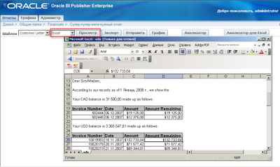

Наверняка, вы сталкивались с минусами такого подхода: невозможность точного форматирования выходной разметки, невозможность задания формата ячейки, невозможность разбиения отчета на листы, невозможность использования макросов, вывода графиков и диаграмм. Список можно продолжать.
Частично выручал метод создания отчетов с помощью XSL-шаблонов разметки, но и там большинство «нельзя» оставалось, плюс мы должны были регламентами использования ограничивать браузер (только IE), версию MS Office (2003 и выше), чтобы полученный отчет прозрачно для пользователя открывался в Экселе.
Прочитать об этом можно на блоге Тима Декстера
Итак, для использования XLS-шаблонов вам в первую очередь потребуется обновить BIPublisher. Для этого скачайте с металинка патч 9546699
Возьмите отформатированный в Экселе шаблон вашего отчета.
Я покажу пример на основе отчета «Balance Letter» из стандартной поставки BIPublisher.

Создайте в нем новый лист с именем XDO_METADATA , на котором поместите общую информацию о шаблоне.
(Не забудьте скрыть затем этот лист.)
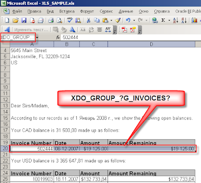
Теперь для каждой ячейки низшей группы задайте имя, соответствующее элементу XML-файла данных.


На данном этапе будем считать наш шаблон разметки завершенным.
Выделенные области пока оставим без изменения.

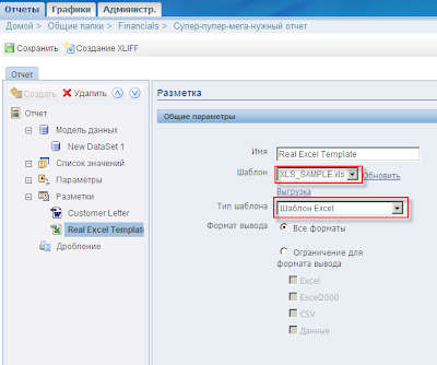
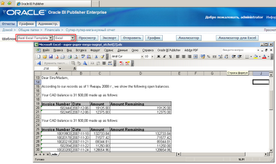

Видим, что остались видны все имена именованных диапазонов исходного шаблона разметки. Именно по ним в итоге полученный XML-файл преобразуется в Excel.
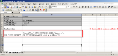
На скрытом листе XDO_METADATA определим новую переменную, значение которой получается конкатенацией статического текста и динамического значения кода валюты и суммы по ней.
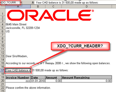
Присвоим первой ячейке в строке имя, равное определенной нами переменной.
Читайте также:
- Excel зависает при копировании ячеек
- Нет напряжения на микросхеме bios
- Чем отличается microsoft office профессиональный плюс от стандартного
- Как создать блестящую кисть в фотошопе
- Как добавить evernote в outlook
Удаление надстройки VBA-Excel
Будем рады Вашей обратной связи
Мы сожалеем, что наша программа не подошла для Вас. Мы стараемся усовершенствовать ее внедряя новый функционал и исправляя выявленные ошибки. Будем рады если Вы дадите нам обратную связь, на основе которой мы поймем в каком направлении нам двигаться.
Оставьте Ваше предложение на этой странице.
Инструкция по отключению надстройки
- Откройте любой файл Excel, либо «чистую» книгу
- Откройте параметры Excel

- Перейдите в список надстроек
- Отключите надстройку VBA-Excel сняв с нее выбор и нажав ОК.
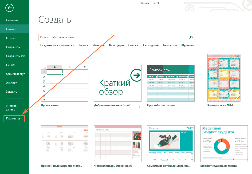
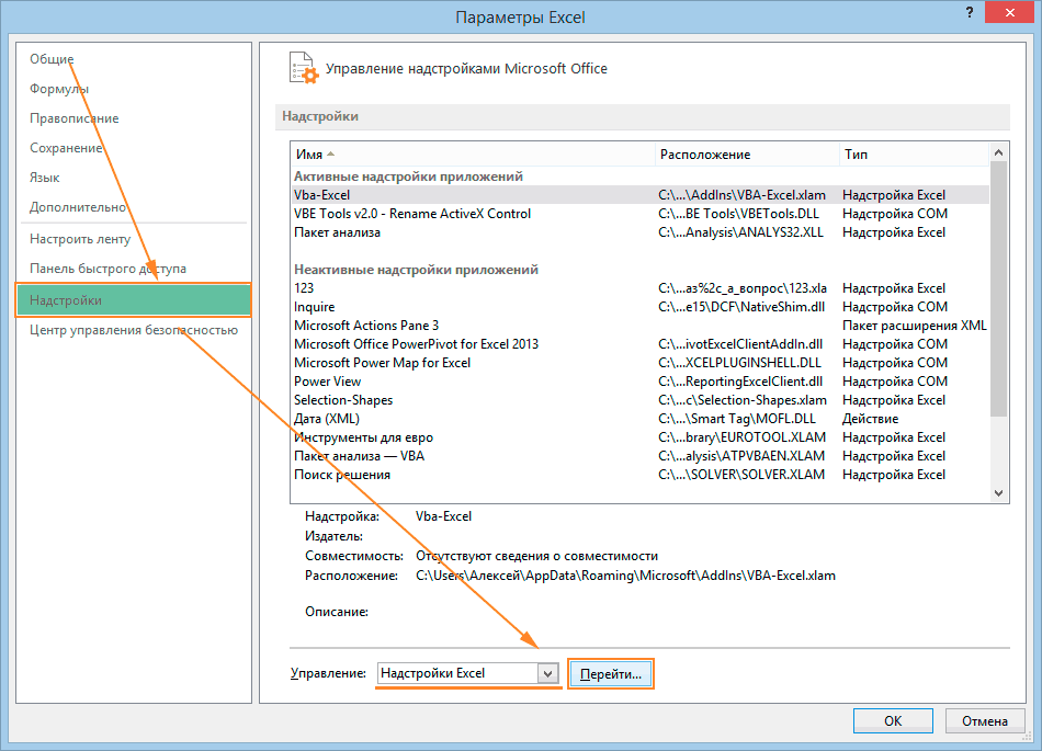
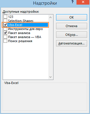
В результате вкладка с надстройкой исчезнет с компьютера и больше не будет загружаться вместе с Excel.
Вы сможете подключить надстройку тогда, когда она понадобиться.
Полное удаление программы
Если Вы больше не планируете пользоваться программой, то помимо отключения надстройки необходимо удалить сам файл с программой. Для этого:
- Откройте диалоговое окно Надстройки повторив действия указанные выше.
- Выделите надстройку VBA-Excel и нажмите Обзор.
- Откроется местоположение файла. Удалите его и программа удалится полностью.
Как удалить надстройку xla/xlam из Excel? Удаление надстроек из списка доступных надстроек
Наверное, у каждого пользователя, активно использующего надстройки, рано или поздно наступает такой момент, когда возникает желание почистить список доступных надстроек, то есть убрать из него все лишнее и неиспользуемое, удалить ставшие ненужными те или иные надстройки или их предыдущие версии, ставшие неактуальными.
Удаление надстроек Excel xla/xlam условно можно разбить на три этапа:
1) Отключение надстройки;
2) удаление файла надстройки;
3) изменение состояния надстройки с последующим удалением ее из списка.
Можно посмотреть видео этого процесса.
Рассмотрим каждый этап подробнее на примере Excel 2007, в других версиях Excel надстройки удаляются аналогично.
Отключение активной надстройки
Перед тем как удалить надстройку Excel xla/xlam, необходимо сделать ее неактивной, то есть отключить. Чтобы узнать состояние надстройки (активная она или нет) необходимо нажать кнопку «Office»  и перейти в «Параметры Excel». Появляется окно «Параметры Excel», где в разделе «Надстройки» виден список всех установленных надстроек, сгруппированных на активные и неактивные. Активные – это те надстройки, которые на данный момент подключены, соответственно неактивные – это те, которые в данный момент отключены. Здесь также можно узнать место расположения файла удаляемой надстройки (оно нам вскоре понадобится). Обратите внимание на скриншот ниже, на нем видны активные надстройки, одну из них с названием test.xla мы и будем удалять.

Удаление файла надстройки
Итак, из приведенного выше окна мы узнали текущее состояние надстройки, которую собираемся удалить. Надстройка test.xla активная, поэтому переходим в поле «Управление», выбираем из списка «Надстройки Excel» и нажимаем кнопку «Перейти». Снимаем флажок перед названием надстройки.

Все, надстройка стала неактивной, мы ее отключили. Теперь можно удалять файл. Место расположения файла мы уже предварительно выяснили чуть раньше, так что осталось зайти в указанную папку и удалить этот файл (можно переместить файл в другую папку или переименовать, если надстройка будет использоваться в будущем). Вот собственно и все, фактически надстройка уже удалена, но она продолжает оставаться в списке доступных надстроек, а в некоторых случаях может и доставлять определенные неудобства, вынуждая Excel при каждом запуске выдавать сообщение с текстом «Не удалось найти файл. Проверьте правильность ввода имени и расположения файла. При попытке открытия файла из списка недавно использованных файлов убедитесь, что файл не был переименован, перемещен или удален».

Изменение состояния надстройки с последующим удалением ее из списка
Для окончательного удаления надстройки из списка доступных надстроек, опять зайдем в окно «Надстройки» и попытаемся изменить состояние надстройки, то есть поставить флажок, если поле пустое, либо снять флажок, если он установлен. При попытке изменения состояния уже удаленной надстройки появится сообщение «Надстройка не найдена. Удалить из списка?».
Добавление и удаление надстроек в Excel
Примечание: Мы стараемся как можно оперативнее обеспечивать вас актуальными справочными материалами на вашем языке. Эта страница переведена автоматически, поэтому ее текст может содержать неточности и грамматические ошибки. Для нас важно, чтобы эта статья была вам полезна. Просим вас уделить пару секунд и сообщить, помогла ли она вам, с помощью кнопок внизу страницы. Для удобства также приводим ссылку на оригинал (на английском языке).
Надстройки расширяют диапазон команд и возможностей Microsoft Excel. По умолчанию они доступны не сразу, поэтому сначала их необходимо установить и (в некоторых случаях) активировать.
Вы ищете сведения о надстройках Office на основе HTML, CSS и JS? В этом случае ознакомьтесь со статьей получение надстройки Office для Excel.
Некоторые надстройки, такие как «Пакет анализа» и «Поиск решения», встроены в Excel. Другие доступны в Центре загрузки, и их необходимо предварительно скачать и установить. Кроме того, некоторые надстройки создаются сторонними организациями, например поставщиками программных решений или программистами. Это могут быть надстройки модели COM, надстройки Visual Basic для приложений (VBA) и надстройки DLL. Они также требуют установки.
Большинство надстроек можно разделить на три типа, описанных ниже.
Надстройки Excel. Обычно к этому типу относят файлы надстроек Excel (XLAM), Excel 97–2003 (XLA) и надстроек DLL (XLL), а также надстройки автоматизации. Некоторые надстройки Excel, такие как «Пакет анализа» и «Поиск решения», становятся доступны после установки Microsoft Office или Excel. Для использования этих надстроек в большинстве случаев нужно лишь активировать их.
Скачиваемые надстройки. Дополнительные надстройки для Excel можно скачать и установить со страницы Загрузки на сайте Office.com.
Пользовательские надстройки. Многие разработчики и поставщики решений создают пользовательские надстройки модели COM, надстройки автоматизации, VBA и XLL. Они требуют установки.
После установки надстройки или ее активации соответствующие команды становятся доступны в одном из указанных ниже мест.
Вкладка Данные. После установки и активации надстроек «Пакет анализа» и «Поиск решения» в группе Анализ становятся доступны команды Анализ данных и Поиск решения.

Вкладка Формулы. После установки и активации инструментов для евро в группе Решения становятся доступны команды Пересчет в евро и Формат евро.
Вкладка Надстройки. Другие надстройки можно добавить на вкладку Надстройки. Эта вкладка добавляется на ленту после установки и активации первой надстройки, которая должна отображаться на ней. Если вкладка надстройки не отображается, необходимо закрыть и перезапустить Excel.
Другие надстройки, такие как вкладка Начало работы, доступны в Excel в других местах, например в виде вкладки на ленте, или через макросы или пользовательские меню.
Важно: С помощью этой процедуры разработчики могут добавлять и удалять надстройки автоматизации перед разработкой программ установки и удаления данных надстроек.
Активация надстройки Excel
На вкладке Файл выберите команду Параметры, а затем — категорию Надстройки.
В поле Управление выберите элемент Надстройки Excel и нажмите кнопку Перейти.
Откроется диалоговое окно Надстройки.
В поле Доступные надстройки установите флажок той надстройки, которую необходимо активировать, а затем нажмите кнопку ОК .
Если в окне Доступные надстройки не удается найти надстройку, которую требуется активировать, возможно, ее требуется установить.
Установка надстройки Excel
Чтобы установить надстройку, которая обычно устанавливается вместе с Excel, например «Пакет анализа» или «Поиск решения», запустите программу установки Excel или Microsoft Office и выберите вариант Изменить, а затем выберите требуемую надстройку. После перезапуска Excel она должна появиться в поле Доступные надстройки.
Некоторые надстройки Excel хранятся на компьютере. Чтобы установить или активировать их, нажмите кнопку Обзор (в диалоговом окне Надстройки), найдите надстройку, а затем нажмите кнопку ОК.
Некоторые надстройки Excel требуют запуска пакета установки. В этом случае может потребоваться загрузить или скопировать пакет установки на компьютер (обычно пакеты установки имеют расширение MSI), а затем запустить его.
Другие надстройки, отсутствующие на компьютере, можно скачать и установить с помощью веб-браузера со страницы Загрузки или с других сайтов в Интернете или на сервере организации. Чтобы скачать их, следуйте инструкциям по установке.
Отключение надстройки Excel
На вкладке Файл выберите команду Параметры, а затем — категорию Надстройки.
В поле Управление выберите элемент Надстройки Excel и нажмите кнопку Перейти.
В поле Доступные надстройки снимите флажок той надстройки, которую нужно деактивировать, а затем нажмите кнопку ОК .
Во многих случаях деактивация надстройки приводит к ее удалению с ленты. В других случаях для удаления надстройки с ленты может потребоваться перезапустить Excel.
Примечание. При деактивации надстройки она не удаляется с компьютера. Чтобы удалить надстройку с компьютера, необходимо воспользоваться средством установки/удаления программ.
Удаление надстройки Excel
Важно: Если надстройка Excel была установлена с сетевого файлового сервера или из общей папки, удалять ее, возможно, потребуется там же. Если надстройка Excel была установлена с компакт-диска, а после установки буква диска для дисковода компакт-дисков была изменена, следует выполнить повторную установку надстройки с компакт-диска. При запуске надстроек Excel с компакт-диска необходимо сначала удалить их с компьютера, а затем выполнить повторную установку с компакт-диска.
Откройте вкладку Файл и выберите пункт Выход.
Выберите в панели управления пункт Программы и компоненты (для Windows 7 и Windows Vista) или Установка и удаление программ (для Windows XP).
Выполните одно из указанных ниже действий.
Если приложение Excel было установлено в составе пакета Microsoft Office, в списке установленных программ выберите пункт Microsoft Office, а затем нажмите кнопку Заменить.
Если приложение Excel было установлено отдельно, в списке установленных программ выберите название программы, а затем нажмите кнопку Заменить.
Если вы установили надстройку из Центра загрузки, выберите имя программы в списке установленных и нажмите кнопку Удалить.
Следуйте инструкциям программы установки.
Важно: С помощью этой процедуры разработчики могут добавлять и удалять надстройки автоматизации перед разработкой программ установки и удаления данных надстроек. Пользователям эта процедура не потребуется. Инструкции по установке и удалению надстройки можно получить у системного администратора, который предоставил эту надстройку.
Добавление надстройки COM
На вкладке Файл выберите команду Параметры, а затем — категорию Надстройки.
В списке Управление нажмите Надстройки COM, а затем — Перейти.
Откроется диалоговое окно Надстройки COM.
В поле Доступные надстройки установите флажок для той надстройки, которую необходимо установить, и нажмите кнопку ОК.
Совет Если нужная надстройка отсутствует в поле Список надстроек, нажмите кнопку Добавить, а затем найдите надстройку.
Удаление надстройки COM
На вкладке Файл выберите команду Параметры, а затем — категорию Надстройки.
В списке Управление нажмите Надстройки COM, а затем — Перейти.
Откроется диалоговое окно Надстройки COM.
В поле Список надстроек снимите флажок той надстройки, которую нужно удалить, а затем нажмите кнопку ОК .
Примечание. В результате надстройка будет удалена из памяти, но ее имя останется в списке доступных надстроек. Надстройка не будет удалена с компьютера.
Чтобы удалить надстройку COM из списка доступных надстроек и с компьютера, щелкните ее имя в поле Список надстроек, а затем нажмите кнопку Удалить.
Примечание: С помощью этой процедуры разработчики могут добавлять и удалять надстройки автоматизации перед разработкой программ установки и удаления данных надстроек. Пользователям эта процедура не потребуется. Инструкции по установке и удалению надстройки можно получить у системного администратора, который предоставил эту надстройку.
На вкладке Файл выберите команду Параметры, а затем — категорию Надстройки.
В поле Управление выберите элемент Надстройки Excel и нажмите кнопку Перейти.
Откроется диалоговое окно Надстройки.
Чтобы установить надстройку автоматизации, в поле Доступные серверы автоматизации выберите пункт Автоматизация и щелкните нужную надстройку.
Совет Если нужной надстройки нет в списке, нажмите кнопку Обзор , найдите нужную надстройку, а затем нажмите кнопку ОК .
Чтобы удалить надстройку автоматизации, ее нужно удалить из реестра. За дополнительными сведениями обратитесь к системному администратору.
Некоторые надстройки, такие как «Пакет анализа» и «Поиск решения», встроены в Excel. Другие доступны в Центре загрузки, и их необходимо предварительно скачать и установить. Кроме того, некоторые надстройки создаются сторонними организациями, например поставщиками программных решений или программистами. Это могут быть надстройки модели COM, надстройки Visual Basic для приложений (VBA) и надстройки DLL. Они также требуют установки.
Большинство надстроек можно разделить на три типа, описанных ниже.
Надстройки Excel. Обычно к этому типу относят файлы надстроек Excel (XLAM), Excel 97–2003 (XLA) и надстроек DLL (XLL), а также надстройки автоматизации. Некоторые надстройки Excel, такие как «Пакет анализа» и «Поиск решения», становятся доступны после установки Microsoft Office или Excel. Для использования этих надстроек в большинстве случаев нужно лишь активировать их.
Скачиваемые надстройки. Дополнительные надстройки для Excel можно скачать и установить со страницы Загрузки на сайте Office.com.
Пользовательские надстройки. Многие разработчики и поставщики решений создают пользовательские надстройки модели COM, надстройки автоматизации, VBA и XLL. Они требуют установки.
После установки надстройки или ее активации соответствующие команды становятся доступны в одном из указанных ниже мест.
Вкладка Данные. После установки и активации надстроек «пакет анализа» и «Поиск решения» команды » анализ данных» и «Поиск решения» доступны на вкладке » данные » на ленте.
Вкладка » Главная «. Другие надстройки можно добавить на вкладку » Главная «.
Другие надстройки, такие как вкладка Начало работы, доступны в Excel в других местах, например в виде вкладки на ленте, или через макросы или пользовательские меню.
Важно: С помощью этой процедуры разработчики могут добавлять и удалять надстройки автоматизации перед разработкой программ установки и удаления данных надстроек.
Активация предварительно установленной надстройки Excel
В меню Сервис выберите пункт надстройки.
В диалоговом окне Доступные надстройки установите флажок для надстройки, которую требуется активировать, и нажмите кнопку ОК.
Установка надстройки Excel
Некоторые надстройки Excel находятся на вашем компьютере и могут быть установлены или активированы с помощью кнопки Обзор (в диалоговом окне » надстройки » выше), чтобы найти надстройку, а затем нажмите кнопку ОК.
Некоторые надстройки Excel требуют запуска пакета установки. В этом случае может потребоваться загрузить или скопировать пакет установки на компьютер (обычно пакеты установки имеют расширение MSI), а затем запустить его.
Другие надстройки, недоступные на вашем компьютере, можно скачать и установить с помощью веб-браузера из загрузок или с других сайтов в Интернете, с сервера в организации или с помощью встроенного параметра » магазин » в Excel. Чтобы скачать их, следуйте инструкциям по установке.
Установка надстроек из магазина
Откройте вкладку Вставка на ленте.
Нажмите кнопку магазин .
Чтобы найти надстройки, используйте поле » категории » или » Поиск «.
Нажмите кнопку Добавить , чтобы установить надстройку.
Примечание: Некоторые надстройки должны быть приобретены.
Удаление надстройки Excel
На вкладке Вставка нажмите кнопку Моинадстройки.
В надстройках Officeщелкните меню 3 точки рядом с надстройкой.
Прочитайте уведомление о других устройствах и нажмите кнопку Удалить.
Отключение надстроек в Microsoft Office 2007
Сведения о вопросе

Надстройка — это устанавливаемый компонент, который добавляет пользовательские команды и новые возможности к приложениям 2007 системы Microsoft Office. Надстройки предназначены для реализации новых или обновленных функций, повышающих производительность труда пользователя.
Вы можете самостоятельно управлять установленными надстройками:
Для Word (Access, Excel, PowerPoint):
- Нажмите кнопку Microsoft Office , затем нажмите кнопку Параметры Word (Access, Excel, PowerPoint) и откройте раздел Надстройки.
- Найдите в поле Надстройки надстройку, которую необходимо включить или отключить, и обратите внимание на тип надстройки в столбце Тип.
- Выберите тип надстройки в поле Управление и нажмите кнопку Перейти.
- Установите или снимите флажок для надстройки, которую необходимо включить или отключить, и нажмите кнопку ОК.
Для Outlook, InfoPath, Publisher, Visio:
- В меню Сервис выберите пункт Центр управления безопасностью и щелкните Надстройки.
- Найдите в поле Надстройки надстройку, которую необходимо включить или отключить, и обратите внимание на тип надстройки в столбце Тип.
- Выберите тип надстройки в поле Управление и нажмите кнопку Перейти.
- Установите или снимите флажок для надстройки, которую необходимо включить или отключить, и нажмите кнопку ОК.
Подключение/отключение надстроек

В основном, данный файл предназначен для подключения/удаления надстроек, выложенных на данном сайте на странице Мои надстройки.
Добавить надстройку — надстройка, выбранная в соответствующем поле, будет добавлена в список доступных надстроек Microsoft Excel и автоматически подключена.
Только для выложенных на сайте надстроек — Если установлен флажок Подключить файл помощи, то так же автоматически файл помощи будет подключен и его можно будет вызвать из надстройки нажатием значка соответствующей команды.
Удалить надстройку -надстройка, выбранная в соответствующем поле, будет удалена и отключена. Так же будет удален файл помощи для данной надстройки.
Только для выложенных на сайте надстроек — Если файл помощи не указан — то будет удален файл, относящейся программно к выбранной для удаления надстройке.
При помощи данного файла можно подключать и удалять абсолютно любые надстройки, а не только выложенные на данном сайте. Просто необходимо будет снять флажок с пункта — Подключить файл помощи.
 MyProgramms_Install_Addins.zip (305,8 KiB, 6 573 скачиваний)
Внимание: программа распространяется бесплатно. Распространение данной программы в коммерческих целях запрещено.
Если решили самостоятельно подключить надстройку(на примере установки MyAddin.xla):
Помещаем файл надстройки с раширением .xla:
- в папку надстроек Excel, как правило она расположена по адресу:
C:Documents and SettingsДмитрийApplication DataMicrosoftAddIns ;
для Windows 7: C:UsersДмитрийAppDataRoamingMicrosoftAddIns - в любое место на локальном диске;
Вместо «Дмитрий» — Ваша учетная запись на компьютере.
Запускаем Excel и выбираем:
- 2010-2016 Excel — Файл—Параметры—Надстройки—Перейти
- 2007 Excel — Меню—Параметры Excel—Надстройки—Перейти

- 2003 Excel — Сервис—Надстройки

Если надстройка была помещена в папку C:Documents and SettingsДмитрийApplication DataMicrosoftAddIns , то она будет отображена в списке и Вам надо будет только выбрать её, поставив галочку. 
Если же Вы поместили надстройку в другую папку, то в окне выбора надстроек нажмите кнопку «Обзор» и выберите файл надстройки. После нажатия «ОК» надстройка будет подключена.
После подключения и установки надстройки для версий Excel 2007 и старше на панели появится новая вкладка(если она еще не отображена) — «Надстройки» (Add-Ins) и на ней будут показаны элементы, относящиеся к данной надстройке. Для версий Excel 2003 и ниже — команды новой надстройки будут созданы вместе с новой панелью, которая должна отобразиться сразу после установки надстройки.
Вкладка «Надстрйоки» и меню появляются только в том случае, если это предусмотрено надстройкой. Если в надстройке не реализован визуальный интерфейс, а присутствуют лишь функции пользователя или процедуры, запускаемые не с панели — то панель не появится.
Microsoft Excel — программа, позволяющая работать с электронными таблицами. Можно собирать, преобразовывать и анализировать данные, проводить визуализацию информации, автоматизировать вычисления и выполнять еще ряд полезных и необходимых в работе задач.
Изучение возможностей Excel может быть полезно в рамках практически любой профессии и сферы деятельности, от работников продаж до бухгалтеров и экономистов.
Возможности Microsoft Excel
Работа с формулами и числовыми данными
Excel может выполнять практически всё: от простых операций вроде сложения, вычитания, умножения и деления до составления бюджетов крупных компаний.
Работа с текстом
Несмотря на то что некоторые возможности Word в Excel неприменимы, программа очень часто является базовой для составления отчетов.
Организация баз данных
Excel — табличный редактор, поэтому систематизация больших архивов не является для него проблемой. Кроме того, благодаря перекрестным ссылкам можно связать между собой различные листы и книги.
Построение графиков и диаграмм
Для создания отчетов очень часто требуется их визуальное представление. В современных версиях Excel можно создать диаграммы и графики любого типа, настроив их по своему усмотрению.
Создание рисунков
С помощью настройки графических объектов, встроенных в программу, можно создавать двухмерные и трехмерные рисунки.
Автоматизация стандартных задач
Excel обладает функцией записи макросов, которые облегчают работу с однотипными действиями. Под любой макрос можно создать отдельную кнопку на рабочей панели или установить сочетание горячих клавиш.
Импорт и экспорт данных
Для создания масштабных отчетов можно загружать данные различных типов со сторонних ресурсов.
Собственный язык программирования
Язык программирования Visual Basic позволяет сделать работу в программе максимально удобной. Большое количество встроенных функций помогают сделать таблицы интерактивными, что упрощает восприятие.
Интерфейс Excel
В настоящий момент самой современной, 16-й версией программы является Excel 2019. Обновления, появляющиеся с каждой новой версией, касаются прежде всего новых формул и функций. Начальный рабочий стол с версии 2007 года претерпел мало изменений.
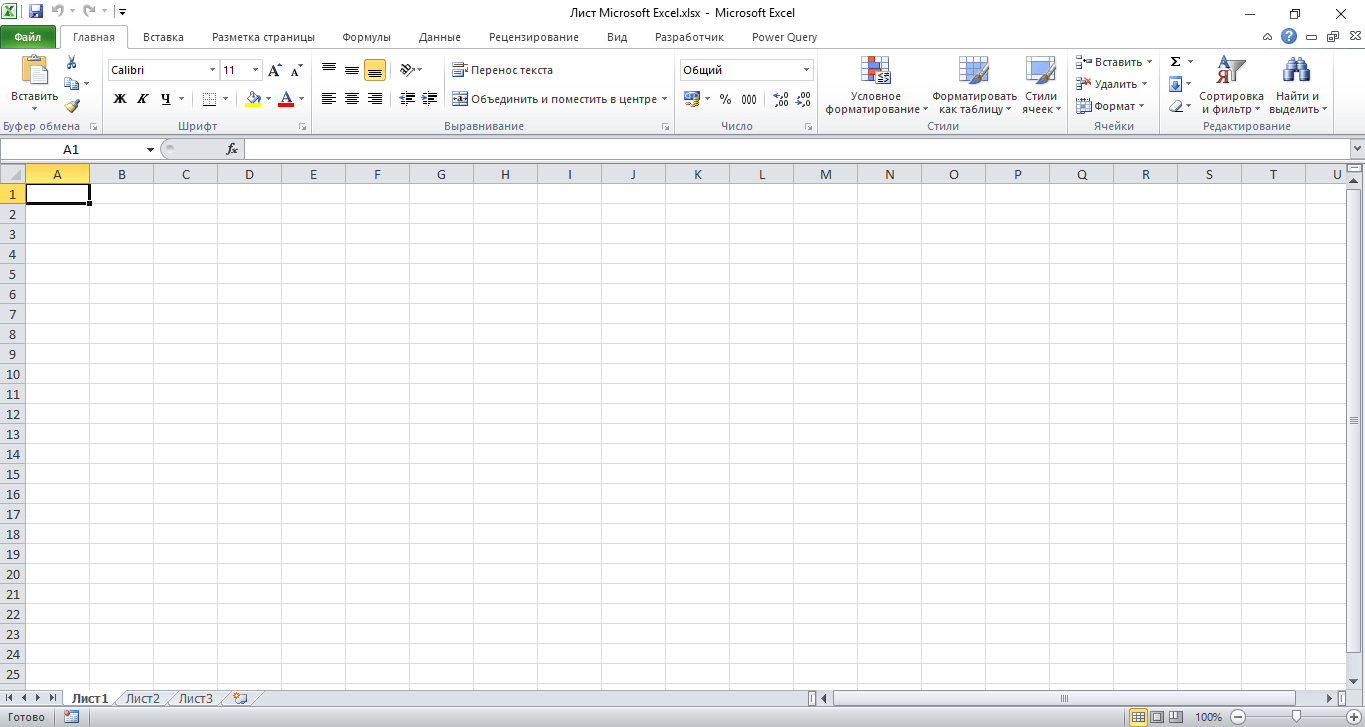
По умолчанию в каждой книге присутствует один лист (в ранних версиях — три листа). Количество листов, которые можно создавать в одной книге, ограничено только возможностями оперативной памяти компьютера. Поле Excel представляет собой таблицу из ячеек. Каждая ячейка имеет свой уникальный адрес, образованный пересечением строк и столбцов. Всего в Excel 1 048 576 строк и 16 384 столбца, что дает 2 147 483 648 ячеек. Над полем с ячейками находится строка функций, в которой отображаются данные, внесенные в ячейки или формулы. Также в программе есть несколько вкладок, которые мы разберем подробнее.
«Файл». С помощью этой вкладки можно отправить документы на печать, установить параметры работы в программе и сделать другие базовые настройки.
«Главная». Здесь располагается основной набор функций: возможность смены параметров шрифта, сортировка данных, простейшие формулы и правила условного форматирования.
«Вставка». Вкладка предназначена для добавления графических элементов на лист. Пользователь может как добавить обычные рисунки и фотографии, так и создать 2D- и 3D-объекты через конструктор. Кроме того, один из самых важных разделов программы — графики и диаграммы — также находится здесь.
«Разметка страницы». Здесь пользователь может менять формат итогового файла, работать с темой и подложкой.
«Формулы». Все формулы и функции, с которыми пользователь может работать в программе, собраны в этой вкладке и рассортированы по соответствующим разделам.
«Данные». Вкладка помогает с фильтрацией текстовых и числовых значений в таблицах, позволяет импортировать данные из других источников.
«Рецензирование». Здесь можно оставлять примечания к ячейкам, а также устанавливать защиту листа и всей книги.
«Вид». На этой вкладке можно добавлять или убирать сетку таблицы, масштабировать значения, закреплять группы данных в таблицах.
«Разработчик». Дополнительная вкладка, которая не включена по умолчанию. Позволяет работать с Visual Basic, создавать новые макросы и запускать уже имеющиеся.
Форматы файлов
Для Excel существует несколько форматов готовых файлов, которые определяют возможности книги:
- .xlsx — стандартная рабочая книга. Пришла на смену бинарному формату .xls с версии 2007 года;
- .xlsm — рабочая книга, позволяющая работать с макросами;
- .xlsb — рабочая книга, использующая бинарный формат, но одновременно и поддерживающая макросы. Обычно используется при работе с большими таблицами;
- .xltm — шаблон-основа для рабочих книг. Имеется поддержка макросов;
- .xlam — надстройка, созданная для добавления дополнительного функционала.
Нужно учитывать, что некоторые формулы и функции из новых версий могут не работать в старых.
Стандартные операции с ячейками
Активной считается ячейка, которая имеет черную рамку выделения с квадратом в правом нижнем углу. Чтобы вносить данные в ячейку, не обязательно делать по ней дополнительные клики мышью. Вносить данные можно как непосредственно в ячейку, так и через строку формул. При перемещении курсора с помощью клавиш-стрелок активной становится соседняя ячейка, текст в предыдущей сохраняется. Чтобы изменить уже имеющийся текст, необходимо дважды кликнуть по ячейке или внести правки через строку формул.
При двойном клике по черному квадрату в правом нижнем углу текстовые данные протянутся до нижнего края созданной таблицы. Если выделить диапазон с последовательными значениями (числа, даты, дни недели), они автоматически пересчитаются в сторону увеличения, заполнив столбец до нижнего края таблицы. Те же операции можно проделать и вручную, протянув за квадрат в нижнем правом углу. В этом случае пользователь самостоятельно определяет границы заполнения.
Чтобы выделить несколько ячеек одновременно, нужно зажать клавишу Ctrl и выбрать нужные ячейки или диапазоны ячеек. Ту же самую операцию можно проделать со строками и столбцами, выделяя необходимое их количество.
Excel автоматически суммирует значения в ячейках, показывая результат в правом нижнем углу листа. Также пользователю предлагаются средние значения данных и общее количество заполненных ячеек.
Ширину столбцов и высоту строк можно менять как вручную, передвигая край столбца/строки, так и нажав правую клавишу мыши и выбрав меню «Ширина столбца (высота строки)». По умолчанию значение ширины указывает на количество символов текущего размера шрифта, которые могут разместиться в ячейке, а значение высоты — на максимально возможный размер шрифта для этой строки.
Ячейки можно объединять с помощью соответствующего меню на вкладке «Главная». Всего существует три варианта объединения:
- объединить и поместить в центре;
- объединить по строкам;
- объединить ячейки.
Следует помнить, что при объединении может нарушаться сортировка данных в таблицах, а также могут некорректно считаться формулы.
Работа с формулами Excel
Главная функция программы — возможность подсчета значений с помощью встроенных формул и функций. Среди них есть простые, позволяющие подсчитать сумму в диапазоне, среднее значение в диапазоне, количество заполненных ячеек и т.д. Есть и более сложные, способные вычислять количество дней между разными датами (в т.ч. рабочих), максимальные и минимальные значения в диапазоне. Работа с функциями и формулами также напрямую зависит от формата ячеек. По умолчанию для всех ячеек установлен общий формат, позволяющий работать как с числовыми, так и с текстовыми данными. Но для более сложной работы он может быть заменен на числовой, процентный, дату, денежный, финансовый, дробный и т.д.
Формула вводится либо через строку функций над таблицей, либо в самой ячейке при двойном клике. В начале функции обязательно должен стоять знак «=». После этого при вводе названия функции появляется помощник, который предлагает выбрать функции из списка. Разберем это на примере формулы средней сложности «СЧЕТЕСЛИ».
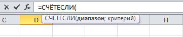
В скобках после функции будут прописаны условия, по которым формула будет проводить вычислениях. Подсказка указывает на то, что потребуется задать диапазон вычислений и критерий, по которому они будут производиться.
Например, нам необходимо подсчитать количество букв «А» в указанном диапазоне:
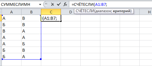
Выделяем диапазон, отмечаем первое условие с помощью знака «;»
Далее выделяем критерий. Его можно прописать вручную, заключив в кавычки; можно выделить ячейку, в которой этот критерий прописан.
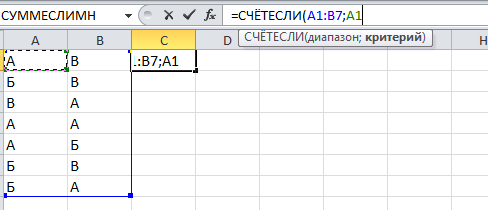
Закрываем скобку, потому что все условия указаны, и нажимаем Enter.
В ячейке C1 получаем ответ: в шести ячейках нашей таблицы написана буква «А».
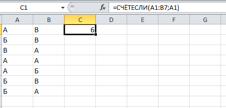
В случае ошибки в формулах в ячейке будет прописано «#ДЕЛ/0!». В этом случае необходимо перепроверить формулу на предмет неточностей и на корректность.
Excel может проводить вычисления не только на активном листе. Для этого при вводе формулы через строку функций нужно перейти на нужный лист и указать ячейку, с которой нужно провести расчет. При протягивании формул автоматически подтянутся и адреса всех ячеек. Чтобы этого не произошло и формулы были подсчитаны корректно, можно закрепить нужную ячейку, выделив ее адрес и нажав клавишу F4. Формат адреса будет выглядеть так: $A$1.