
Excel for Microsoft 365 for Mac Excel 2021 for Mac Excel 2019 for Mac Excel 2016 for Mac Excel for Mac 2011 More…Less
You can use number formats to change the appearance of numbers, including dates and times, without changing the actual number. The number format does not affect the cell value that Excel uses to perform calculations. The actual value is displayed in the formula bar.
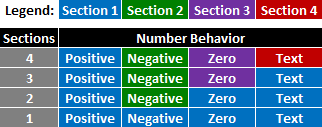
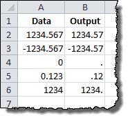
Excel provides several built-in number formats. You can use these built-in formats as is, or you can use them as a basis for creating your own custom number formats. When you create custom number formats, you can specify up to four sections of format code. These sections of code define the formats for positive numbers, negative numbers, zero values, and text, in that order. The sections of code must be separated by semicolons (;).
The following example shows the four types of format code sections.

 Format for positive numbers
 Format for negative numbers
 Format for zeros
 Format for text
If you specify only one section of format code, the code in that section is used for all numbers. If you specify two sections of format code, the first section of code is used for positive numbers and zeros, and the second section of code is used for negative numbers. When you skip code sections in your number format, you must include a semicolon for each of the missing sections of code. You can use the ampersand (&) text operator to join, or concatenate, two values.
Create a custom format code
-
On the Home tab, click Number Format
 , and then click More Number Formats.
 -
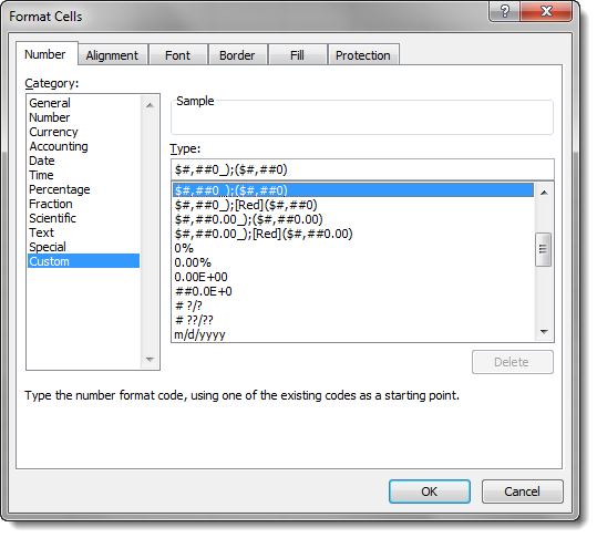
In the Format Cells dialog box, in the Category box, click Custom.
-
In the Type list, select the number format that you want to customize.
The number format that you select appears in the Type box at the top of the list.
-
In the Type box, make the necessary changes to the selected number format.
Format code guidelines
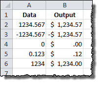
To display both text and numbers in a cell, enclose the text characters in double quotation marks (» «) or precede a single character with a backslash (). Include the characters in the appropriate section of the format codes. For example, you could type the format $0.00″ Surplus»;$–0.00″ Shortage» to display a positive amount as «$125.74 Surplus» and a negative amount as «$–125.74 Shortage.»
You don’t have to use quotation marks to display the characters listed in the following table:
|
Character |
Name |
|
$ |
Dollar sign |
|
+ |
Plus sign |
|
— |
Minus sign |
|
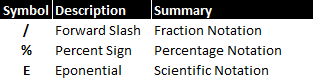
/ |
Forward slash |
|
( |
Left parenthesis |
|
) |
Right parenthesis |
|
: |
Colon |
|
! |
Exclamation point |
|
^ |
Circumflex accent (caret) |
|
& |
Ampersand |
|
‘ |
Apostrophe |
|
~ |
Tilde |
|
{ |
Left curly bracket |
|
} |
Right curly bracket |
|
< |
Less than sign |
|
> |
Greater than sign |
|
= |
Equal sign |
|
Space character |
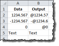
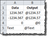
To create a number format that includes text that is typed in a cell, insert an «at» sign (@) in the text section of the number format code section at the point where you want the typed text to be displayed in the cell. If the @ character is not included in the text section of the number format, any text that you type in the cell is not displayed; only numbers are displayed. You can also create a number format that combines specific text characters with the text that is typed in the cell. To do this, enter the specific text characters that you want before the @ character, after the @ character, or both. Then, enclose the text characters that you entered in double quotation marks (» «). For example, to include text before the text that’s typed in the cell, enter «gross receipts for «@ in the text section of the number format code.
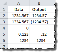
To create a space that is the width of a character in a number format, insert an underscore (_) followed by the character. For example, if you want positive numbers to line up correctly with negative numbers that are enclosed in parentheses, insert an underscore at the end of the positive number format followed by a right parenthesis character.
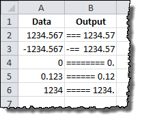
To repeat a character in the number format so that the width of the number fills the column, precede the character with an asterisk (*) in the format code. For example, you can type 0*– to include enough dashes after a number to fill the cell, or you can type *0 before any format to include leading zeros.
You can use number format codes to control the display of digits before and after the decimal place. Use the number sign (#) if you want to display only the significant digits in a number. This sign does not allow the display non-significant zeros. Use the numerical character for zero (0) if you want to display non-significant zeros when a number might have fewer digits than have been specified in the format code. Use a question mark (?) if you want to add spaces for non-significant zeros on either side of the decimal point so that the decimal points align when they are formatted with a fixed-width font, such as Courier New. You can also use the question mark (?) to display fractions that have varying numbers of digits in the numerator and denominator.
If a number has more digits to the left of the decimal point than there are placeholders in the format code, the extra digits are displayed in the cell. However, if a number has more digits to the right of the decimal point than there are placeholders in the format code, the number is rounded off to the same number of decimal places as there are placeholders. If the format code contains only number signs (#) to the left of the decimal point, numbers with a value of less than 1 begin with the decimal point, not with a zero followed by a decimal point.
|
To display |
As |
Use this code |
|
1234.59 |
1234.6 |
####.# |
|
8.9 |
8.900 |
#.000 |
|
.631 |
0.6 |
0.# |
|
12 1234.568 |
12.0 1234.57 |
#.0# |
|
Number: 44.398 102.65 2.8 |
Decimal points aligned: 44.398 102.65 2.8 |
???.??? |
|
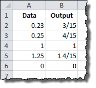
Number: 5.25 5.3 |
Numerators of fractions aligned: 5 1/4 5 3/10 |
# ???/??? |
To display a comma as a thousands separator or to scale a number by a multiple of 1000, include a comma (,) in the code for the number format.
|
To display |
As |
Use this code |
|
12000 |
12,000 |
#,### |
|
12000 |
12 |
#, |
|
12200000 |
12.2 |
0.0,, |
To display leading and trailing zeros prior to or after a whole number, use the codes in the following table.
|
To display |
As |
Use this code |
|
12 123 |
00012 00123 |
00000 |
|
12 123 |
00012 000123 |
«000»# |
|
123 |
0123 |
«0»# |
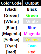
To specify the color for a section in the format code, type the name of one of the following eight colors in the code and enclose the name in square brackets as shown. The color code must be the first item in the code section.
[Black] [Blue] [Cyan] [Green] [Magenta] [Red] [White] [Yellow]
To indicate that a number format will be applied only if the number meets a condition that you have specified, enclose the condition in square brackets. The condition consists of a comparison operator and a value. For example, the following number format will display numbers that are less than or equal to 100 in a red font and numbers that are greater than 100 in a blue font.
[Red][<=100];[Blue][>100]
To hide zeros or to hide all values in cells, create a custom format by using the codes below. The hidden values appear only in the formula bar. The values are not printed when you print your sheet. To display the hidden values again, change the format to the General number format or to an appropriate date or time format.
|
To hide |
Use this code |
|
Zero values |
0;–0;;@ |
|
All values |
;;; (three semicolons) |
Use the following keyboard shortcuts to enter the following currency symbols in the Type box.
|
To enter |
Press these keys |
|
¢ (cents) |
OPTION + 4 |
|
£ (pounds) |
OPTION + 3 |
|
¥ (yen) |
OPTION + Y |
|
€ (euro) |
OPTION + SHIFT + 2 |
The regional settings for currency determine the position of the currency symbol (that is, whether the symbol appears before or after the number and whether a space separates the symbol and the number). The regional settings also determine the decimal symbol and the thousands separator. You can control these settings by using the Mac OS X International system preferences.
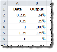
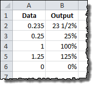
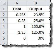
To display numbers as a percentage of 100 — for example, to display .08 as 8% or 2.8 as 280% — include the percent sign (%) in the number format.
To display numbers in scientific notation, use one of the exponent codes in the number format code — for example, E–, E+, e–, or e+. If a number format code section contains a zero (0) or number sign (#) to the right of an exponent code, Excel displays the number in scientific notation and inserts an «E» or «e». The number of zeros or number signs to the right of a code determines the number of digits in the exponent. The codes «E–» or «e–» place a minus sign (-) by negative exponents. The codes «E+» or «e+» place a minus sign (-) by negative exponents and a plus sign (+) by positive exponents.
To format dates and times, use the following codes.
Important: If you use the «m» or «mm» code immediately after the «h» or «hh» code (for hours) or immediately before the «ss» code (for seconds), Excel displays minutes instead of the month.
|
To display |
As |
Use this code |
|
Years |
00-99 |
yy |
|
Years |
1900-9999 |
yyyy |
|
Months |
1-12 |
m |
|
Months |
01-12 |
mm |
|
Months |
Jan-Dec |
mmm |
|
Months |
January-December |
mmmm |
|
Months |
J-D |
mmmmm |
|
Days |
1-31 |
d |
|
Days |
01-31 |
dd |
|
Days |
Sun-Sat |
ddd |
|
Days |
Sunday-Saturday |
dddd |
|
Hours |
0-23 |
h |
|
Hours |
00-23 |
hh |
|
Minutes |
0-59 |
m |
|
Minutes |
00-59 |
mm |
|
Seconds |
0-59 |
s |
|
Seconds |
00-59 |
ss |
|
Time |
4 AM |
h AM/PM |
|
Time |
4:36 PM |
h:mm AM/PM |
|
Time |
4:36:03 PM |
h:mm:ss A/P |
|
Time |
4:36:03.75 PM |
h:mm:ss.00 |
|
Elapsed time (hours and minutes) |
1:02 |
[h]:mm |
|
Elapsed time (minutes and seconds) |
62:16 |
[mm]:ss |
|
Elapsed time (seconds and hundredths) |
3735.80 |
[ss].00 |
Note: If the format contains AM or PM, the hour is based on the 12-hour clock, where «AM» or «A» indicates times from midnight until noon and «PM» or «P» indicates times from noon until midnight. Otherwise, the hour is based on the 24-hour clock.
See also
Create and apply a custom number format
Display numbers as postal codes, Social Security numbers, or phone numbers
Display dates, times, currency, fractions, or percentages
Highlight patterns and trends with conditional formatting
Display or hide zero values
Need more help?
Содержание
- Format numbers as text
- Available number formats in Excel
- Number formats
- Need more help?
- Number format codes
- Create a custom format code
- Format code guidelines
Format numbers as text
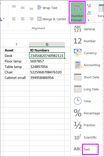
If you want Excel to treat certain types of numbers as text, you can use the text format instead of a number format. For example, If you are using credit card numbers, or other number codes that contain 16 digits or more, you must use a text format. That’s because Excel has a maximum of 15 digits of precision and will round any numbers that follow the 15th digit down to zero, which probably isn’t what you want to happen.
It’s easy to tell at a glance if a number is formatted as text, because it will be left-aligned instead of right-aligned in the cell.
Select the cell or range of cells that contains the numbers that you want to format as text. How to select cells or a range.
Tip: You can also select empty cells, and then enter numbers after you format the cells as text. Those numbers will be formatted as text.
On the Home tab, in the Number group, click the arrow next to the Number Format box, and then click Text.
Note: If you don’t see the Text option, use the scroll bar to scroll to the end of the list.
To use decimal places in numbers that are stored as text, you may need to include the decimal points when you type the numbers.
When you enter a number that begins with a zero—for example, a product code—Excel will delete the zero by default. If this is not what you want, you can create a custom number format that forces Excel to retain the leading zero. For example, if you’re typing or pasting ten-digit product codes in a worksheet, Excel will change numbers like 0784367998 to 784367998. In this case, you could create a custom number format consisting of the code 0000000000, which forces Excel to display all ten digits of the product code, including the leading zero. For more information about this issue, see Create or delete a custom number format and Keep leading zeros in number codes.
Occasionally, numbers might be formatted and stored in cells as text, which later can cause problems with calculations or produce confusing sort orders. This sometimes happens when you import or copy numbers from a database or other data source. In this scenario, you must convert the numbers stored as text back to numbers. For more information, see Convert numbers stored as text to numbers.
You can also use the TEXT function to convert a number to text in a specific number format. For examples of this technique, see Keep leading zeros in number codes. For information about using the TEXT function, see TEXT function.
Источник
Available number formats in Excel
In Excel, you can format numbers in cells for things like currency, percentages, decimals, dates, phone numbers, or social security numbers.

Select a cell or a cell range.
On the Home tab, select Number from the drop-down.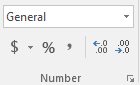
Or, you can choose one of these options:
Press CTRL + 1 and select Number.
Right-click the cell or cell range, select Format Cells… , and select Number.
Select the small arrow, dialog box launcher, and then select Number.
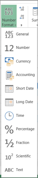
Select the format you want.
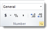
Number formats
To see all available number formats, click the Dialog Box Launcher next to Number on the Home tab in the Number group.

The default number format that Excel applies when you type a number. For the most part, numbers that are formatted with the General format are displayed just the way you type them. However, if the cell is not wide enough to show the entire number, the General format rounds the numbers with decimals. The General number format also uses scientific (exponential) notation for large numbers (12 or more digits).
Used for the general display of numbers. You can specify the number of decimal places that you want to use, whether you want to use a thousands separator, and how you want to display negative numbers.
Used for general monetary values and displays the default currency symbol with numbers. You can specify the number of decimal places that you want to use, whether you want to use a thousands separator, and how you want to display negative numbers.
Also used for monetary values, but it aligns the currency symbols and decimal points of numbers in a column.
Displays date and time serial numbers as date values, according to the type and locale (location) that you specify. Date formats that begin with an asterisk ( *) respond to changes in regional date and time settings that are specified in Control Panel. Formats without an asterisk are not affected by Control Panel settings.
Displays date and time serial numbers as time values, according to the type and locale (location) that you specify. Time formats that begin with an asterisk ( *) respond to changes in regional date and time settings that are specified in Control Panel. Formats without an asterisk are not affected by Control Panel settings.
Multiplies the cell value by 100 and displays the result with a percent ( %) symbol. You can specify the number of decimal places that you want to use.
Displays a number as a fraction, according to the type of fraction that you specify.
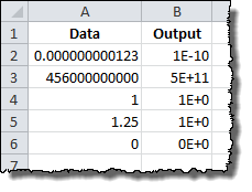
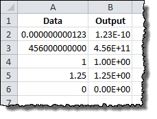
Displays a number in exponential notation, replacing part of the number with E+n, where E (which stands for Exponent) multiplies the preceding number by 10 to the nth power. For example, a 2-decimal Scientific format displays 12345678901 as 1.23E+10, which is 1.23 times 10 to the 10th power. You can specify the number of decimal places that you want to use.
Treats the content of a cell as text and displays the content exactly as you type it, even when you type numbers.
Displays a number as a postal code (ZIP Code), phone number, or Social Security number.
Allows you to modify a copy of an existing number format code. Use this format to create a custom number format that is added to the list of number format codes. You can add between 200 and 250 custom number formats, depending on the language version of Excel that is installed on your computer. For more information about custom formats, see Create or delete a custom number format.
You can apply different formats to numbers to change how they appear. The formats only change how the numbers are displayed and don’t affect the values. For example, if you want a number to show as currency, you’d click the cell with the number value > Currency.
Applying a number format only changes how the number is displayed and doesn’t affect cell values that’s used to perform calculations. You can see the actual value in the formula bar.

Here’s a list of available number formats and how you can use them in Excel for the web:
Default number format. If the cell isn’t wide enough to show the entire number, this format rounds the number. For example, 25.76 shows as 26.
Also, if the number is 12 or more digits, General format displays the value with scientific (exponential) notation.
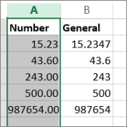
Works very much like the General format but varies how it shows numbers with decimal place separators and negative numbers. Here are some examples of how both formats display numbers:
Shows a monetary symbol with numbers. You can specify the number of decimal places with Increase Decimal or Decrease Decimal.
Also used for monetary values, but aligns the currency symbols and decimal points of numbers in a column.
Shows date in this format:
Shows month, day and year in this format:
Shows number date and time serial numbers as time values.
Multiplies the cell value by 100 and displays the result with a percent ( %) symbol.
Use Increase Decimal or Decrease Decimal to specify the number of decimal places you want.
Shows the number as a fraction. For example, 0.5 displays as ½.
Displays numbers in exponential notation, replacing part of the number with E+ n, where E (Exponent) multiplies the preceding number by 10 to the nth power. For example, a 2-decimal Scientific format displays 12345678901 as 1.23E+10, which is 1.23 times 10 to the 10th power. To specify the number of decimal places you want to use, apply Increase Decimal or Decrease Decimal.
Treats the cell value as text and displays it exactly as you type it, even when you type numbers. Learn more about formatting numbers as text.
Need more help?
You can always ask an expert in the Excel Tech Community or get support in the Answers community.
Источник
Number format codes
You can use number formats to change the appearance of numbers, including dates and times, without changing the actual number. The number format does not affect the cell value that Excel uses to perform calculations. The actual value is displayed in the formula bar.
Excel provides several built-in number formats. You can use these built-in formats as is, or you can use them as a basis for creating your own custom number formats. When you create custom number formats, you can specify up to four sections of format code. These sections of code define the formats for positive numbers, negative numbers, zero values, and text, in that order. The sections of code must be separated by semicolons (;).
The following example shows the four types of format code sections.
Format for positive numbers
Format for negative numbers
Format for zeros
Format for text
If you specify only one section of format code, the code in that section is used for all numbers. If you specify two sections of format code, the first section of code is used for positive numbers and zeros, and the second section of code is used for negative numbers. When you skip code sections in your number format, you must include a semicolon for each of the missing sections of code. You can use the ampersand (&) text operator to join, or concatenate, two values.
Create a custom format code
On the Home tab, click Number Format  , and then click More Number Formats.
In the Format Cells dialog box, in the Category box, click Custom.
In the Type list, select the number format that you want to customize.
The number format that you select appears in the Type box at the top of the list.
In the Type box, make the necessary changes to the selected number format.
Format code guidelines
To display both text and numbers in a cell, enclose the text characters in double quotation marks (» «) or precede a single character with a backslash (). Include the characters in the appropriate section of the format codes. For example, you could type the format $0.00″ Surplus»;$–0.00″ Shortage» to display a positive amount as «$125.74 Surplus» and a negative amount as «$–125.74 Shortage.»
You don’t have to use quotation marks to display the characters listed in the following table:
Circumflex accent (caret)
Left curly bracket
Right curly bracket
Greater than sign
To create a number format that includes text that is typed in a cell, insert an «at» sign (@) in the text section of the number format code section at the point where you want the typed text to be displayed in the cell. If the @ character is not included in the text section of the number format, any text that you type in the cell is not displayed; only numbers are displayed. You can also create a number format that combines specific text characters with the text that is typed in the cell. To do this, enter the specific text characters that you want before the @ character, after the @ character, or both. Then, enclose the text characters that you entered in double quotation marks (» «). For example, to include text before the text that’s typed in the cell, enter «gross receipts for «@ in the text section of the number format code.
To create a space that is the width of a character in a number format, insert an underscore (_) followed by the character. For example, if you want positive numbers to line up correctly with negative numbers that are enclosed in parentheses, insert an underscore at the end of the positive number format followed by a right parenthesis character.
To repeat a character in the number format so that the width of the number fills the column, precede the character with an asterisk (*) in the format code. For example, you can type 0*– to include enough dashes after a number to fill the cell, or you can type *0 before any format to include leading zeros.
You can use number format codes to control the display of digits before and after the decimal place. Use the number sign (#) if you want to display only the significant digits in a number. This sign does not allow the display non-significant zeros. Use the numerical character for zero (0) if you want to display non-significant zeros when a number might have fewer digits than have been specified in the format code. Use a question mark (?) if you want to add spaces for non-significant zeros on either side of the decimal point so that the decimal points align when they are formatted with a fixed-width font, such as Courier New. You can also use the question mark (?) to display fractions that have varying numbers of digits in the numerator and denominator.
If a number has more digits to the left of the decimal point than there are placeholders in the format code, the extra digits are displayed in the cell. However, if a number has more digits to the right of the decimal point than there are placeholders in the format code, the number is rounded off to the same number of decimal places as there are placeholders. If the format code contains only number signs (#) to the left of the decimal point, numbers with a value of less than 1 begin with the decimal point, not with a zero followed by a decimal point.
Источник
December 08, 2019/
Chris Newman
What Are Custom Number Formats?
I love to explain number formats in Excel as the “clothing” of a spreadsheet cell. You can dress your cell values in any way you’d like but even though the outward appearance is different, the underlying value never changes.
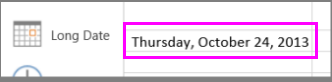
This concept is used most frequently with dates:
Did you know that a date is actually just a numerical number at its core? You can see the true value of the date used in the above example by looking at the “General” format result. However, most people dress this number up to look like a date with forward-slashes.
4 Parts of a Number Format Rule
There are four parts or sections to a Custom Number Format rule. The first section is required while the additional three are optional. Each section is divided up by the use of a semi-colon ( ; ). Here is what each part of the number format rule represents:
-
If the number is positive then do this…
-
If the number is negative then do this…
-
If the number equals zero then do this…
-
If the value is not a number then do this…
A Few Caveats
-
If only the first section has a format rule, it will be applied to all numerical values whether positive or negative (text values will be left alone)
-
If only the first two sections have format rules, zero values will use the positive value format
Using the Number Format Editor
In order to write your own custom number format rules, you will need to navigate to the rule editor. The editor resides within the Format Cells dialog box where you can modify all the properties/formats of a cell.
There are multiple ways to navigate to the Format Cells dialog box:
-
[Method 1] Right-click on cell >> Select Format Cells…
-
[Method 2] Home Tab >> Number Button group >> click Grey Arrow in bottom corner
-
[Method 3] Use the Keyboard Shortcut: ctrl + 1 (PC) | cmd + 1 (Mac)
Once you have opened the Format Cells dialog box, you will want to navigate to the Number tab. This tab will show you a bunch of preset number format rules you can navigate through or if you would like to write your own rule, you can navigate all the way to the bottom of the Category Pane and click Custom.
Special Characters & What They Do
There are a few special characters you can utilize while writing a Custom Number Format rule to add even more varieties to your value’s appearance. Let’s first look at the special characters available to you and then we will get into some examples.
| Character | What It Does |
|---|---|
| @ | A placeholder for text |
| , | Separates thousands |
| * | Repeats character immediately following it |
| 0 | Forces the display of a numerical value |
| # | Placeholder for an optional digit |
| ? | Used to align digits at various lengths |
| _ | Add a space sized as the character immediately following it |
Just by including one of these symbols, your Custom Number Format rule will automatically use its special ability. If you wish to include one of these symbols without their ability, see how to do so in the “Escaping” section of this article (scroll down a few sections).
@ Symbol
The @ symbol is used to control where your text value shows up in your rule. You can place modifications to your text value before or after your text via relocating the @ symbol within the rule.
Comma Symbol
The comma symbol can be used to separate your numbers in thousands or to round large numbers to a specific place (Millions, Billions, etc…).
If you place a comma in front of your “ones” place, you will gain the ability to see a comma separate your value every three places. You only need to use a single comma in order to trigger this format.
If you place a comma behind your “ones” place, the value will VISUALLY lose three places (essentially dividing 1,000). This behavior continues to occur for each additional comma you add behind your “ones” place.
Asterisk Symbol
An asterisk symbol can be used to fill the remaining space within a cell with the character immediately following it. I’ve typically only seen this done when someone is creating a contact list where they would like dots to connect the values in column 1 and column 2.
Zero Number
Using a zero in a number format rule will force that number place to be shown visually. If you would like all your numbers to show three digits, insert three zeros into your rule and 1 will equal 001. This can be very usual in cleaning up your numerical values to ensure they all visually align with one another.
Pound/Hash Symbol
The pound (or hash) symbol serves as an optional placeholder for digits if they exist. If you value exceeds the number of pound signs to the right of your decimal, the format rule will round your value to align with your designated amount of pound symbols. If your value has less digits than pound symbols, a zero will not populate in its place.
Question Mark Symbol
Question marks can be used to align digits when you don’t necessarily want zeros to show up as numerical placeholders. When a question mark resides in a place where no value is provided, a space will be added (shown in grey below) to maintain the alignment of the number.
Underscore Symbol
By using the underscore symbol you can add a single space either before or after your cell value. The character immediately following the underscore determines the size of the space. In most cases, Excel users use the underscore symbol to line up positive and negative numbers that use parenthesis.
Escaping Special Characters
There may be instances where you literally want to use one of the above characters instead of utilizing their special abilities. To remove the special ability (or “escape” the ability), just place a back-slash before the character. You’ll need to place a backslash before each individual symbol you wish to escape.
Adding Text
There may be occasions when you would like to add text before or after your values but still would like to perform spreadsheet math with your data. With Custom Number Format rules, we can easily accomplish making numerical values appear as text visuals while maintaining their cell value.

About The Author
Hey there! I’m Chris and I run TheSpreadsheetGuru website in my spare time. By day, I’m actually a finance professional who relies on Microsoft Excel quite heavily in the corporate world. I love taking the things I learn in the “real world” and sharing them with everyone here on this site so that you too can become a spreadsheet guru at your company.
Through my years in the corporate world, I’ve been able to pick up on opportunities to make working with Excel better and have built a variety of Excel add-ins, from inserting tickmark symbols to automating copy/pasting from Excel to PowerPoint. If you’d like to keep up to date with the latest Excel news and directly get emailed the most meaningful Excel tips I’ve learned over the years, you can sign up for my free newsletters. I hope I was able to provide you with some value today and I hope to see you back here soon!
— Chris
Founder, TheSpreadsheetGuru.com
Number Formatting in Excel: Step-by-Step Tutorial (2023)
We all know how to apply the basic numeric and text formats to cells in Excel.
But do you know how you can add a desired number of decimals, scientific notations, currency symbols, and similar formats in Excel with only a click?
No? This article is for you. It delves into the details of number formatting in Excel. 🤩
Keep reading till the end, and download our free sample workbook here before you scroll down.
What are number formats?
Type something into a cell. What is its format?

By default, all cells of Excel will have the General format applied.
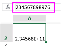
However, type in a big number that exceeds the size of the cell, and Excel would give you back something like 1.2E+12.

What is this? A scientific notation. Under General format, Excel replaces a number too big to fit the cell with its scientific notation.
To turn it into a number, change the format to ‘Numbers’ and adjust the cell size.

Check the formula bar to note how the number remains the same under both formats i.e. 1200000000000.
What changes is only the visual representation of the said number in Excel (decimal places added).
That is how formats work in Excel.
And you can change the format of a number with a mere click. Excel offers many number formats with useful variations to them.
Thousands separator
In the image below we have different numbers.

By now, it only seems like a number that is hard to read. Maybe that’s because it doesn’t yet have 1000s separators (any commas) to it.
- Select the cell.
- Go to Home > Number

- From the menu, go to More Number Formats

This launches the Format Cells dialog box.
You may use the keyboard shortcut (Control Key + 1) to launch the Format Cells dialog box.

- Go to Number Format.
- Check the ‘Use 1000 Separator’ box.

- Here are the results.

A shortcut to add the 1000s separator: Go to Home > Number > click on the comma symbol

However, this changes the number format to the Accounting format.

Controlling decimals
In the same example, as above, there are two decimals to the number.

But you want four decimal places to this number. How can this be done?
- Select the cell.
- Go to Home > Number > More Number Formats

- From the Format Cells dialog box, go to Number Format.
- Adjust the decimal places to four.

- Here are the results.

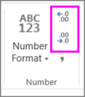
A shortcut to adjust decimal places. Go to Home > Number > Add decimals button

With every click, Excel adds another decimal position to the number.
The button with a right-headed arrow reduces a decimal position.
The button with a left-headed arrow adds a decimal position.
Show as percentage
Here is a decimal number that we want to be converted into a percentage.

To do this:
- Select the cell.
- Go to Home > Number > More Number Formats

- From the Format Cells dialog box, go to Number Format.
- Click on Percentage.

- Adjust the decimal places as desired.

- Here are the results.

A shortcut to convert a number into a percentage. Go to Home > Number > Click the % symbol

Number formatting presets
Excel offers a wide variety of number formatting presets. (You must’ve had a slight idea of that by now.)
These range from currency to accounting to dates and whatnot.
Let’s look into each of these formats below.
General number format preset
The general number format of Excel is the default format of any value in Excel.
All values in all cells of Excel will have the general number format by default.
- To apply the general format to any cell in Excel, select that cell.
- Press the Control key + 1 to launch the Format cells dialog box. That’s a handy shortcut 😊.
- Choose the ‘General number’ format.

- Values formatted as general numbers are displayed just the way they are.
Pro Tip!
Under the General number format, if the cell is not wide enough to contain a number, Excel would:
- Round a number with decimals to lesser decimal places; or
- Use scientific notation to express the number; or
- If the cell is too small to fit in the scientific notation for the number even, display a series of hashes only.
Number format preset
The Excel number format is used for simple numeric values
To apply the number format to any cell:
- Select the cell.
- Go to Home > Numbers > Drop Down Menu and click on Number Format.

The number format allows users three further variations to the final value:
- The decimal places. You can adjust decimal places to any desired number.

- The 1000 Separator. Check the box if you need 1000s separators to the value.

- The format of negative numbers. This could be in two colors (black or red) and enclosed within brackets or with a minus sign.

The Sample box gives a preview of what the final value may look like.

Must Note:
Under the Numbers format, if you type a number in a cell that is too big to fit in the cell, Excel might return a series of hashes only.

In such a case, one must know that the problem simply lies within the size of the cell. (that is too small to fit in the cell value).
To work this out, increase the width of the column until it is wide enough to fit in the cell value.

Currency format preset
The Currency format is used to denote currencies.
To format a number as currency:
- Go to Home > Numbers > Drop Down Menu > Click on Currency.

It allows you to adjust three options to your desire:
- The decimal places.

- The currency symbol.

- The format of negative numbers. This could be in two colors (black or red) and enclosed within brackets or with a minus sign.

Here is what a currency formatted number looks like.

Date format presets
There are two date formats offered by Excel – short date and long date.

To format a number as a date, go to Format Cells and choose the date format you’d want to be applied.

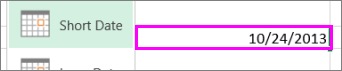
Excel offers a wide variety of formats for dates and days.
Here is how the date format works.

Pro Tip!
Type any number into Excel and apply the date formatting to it. Excel turns it into a date.
This is because Excel recognizes each date as a number. Where 1 is equal to 01 Jan 1900, 2 is equal to 02 Jan 1900, and so on.
Accounting format preset
Next is the accounting format preset.
This format is relevant when you’re working with financial data. For example, while preparing financial statements, forecasts, or similar reports.
To apply accounting format to a number:
- Go to Home > Numbers > Drop Down Menu > Click on Accounting Format.

It allows you to adjust two features to your desire:
- The decimal places.

- The currency symbol.

Here is what an accounting formatted number looks like.

Under the accounting format, 1000s separators and currency symbols are added by default. And negative numbers are enclosed in parenthesis i.e. $ (1925.60) etc.
Time format preset
Excel also offers a wide variety of ways how you may represent times in Excel.
To apply the time format, go to Format Cells and choose the time format you’d want to apply.

You can format it to be displayed as HH:MM:SS or any other way you like.
Here is how the time format looks in action.

Formatting shortcuts
There are plenty of shortcuts on how you may quickly format cell values in Excel.
You can format numbers by using these keyboard shortcuts. Simply select the cell (or cells) where you want the formatting applied and use the shortcuts below.
- Control Key + Shift Key + ~ : Applies the General format
- Control Key + Shift Key + ! : Applies the Number format
- Control Key + Shift Key + $ : Applies the Currency format
- Control Key + Shift Key + % : Applies the Percentage format
- Control Key + Shift Key + ^ : Applies the Scientific notation format
- Control Key + Shift Key + # : Applies the Date format
- Control Key + Shift Key + @ : Applies the Time format
All of these are shortcut keys and only apply the default formats (like the default two decimal places or HH:MM:SS AM/PM format etc.)
Custom formatting
Tired already? However, the number formats list has yet not come to an end.
The last and the most important number format of Excel is the Custom Format.
Under this format, you can customize a number format as needed.
- Go to Home > Numbers > Drop Down Menu > More Number Formats.
- Click on Custom Format.

- Under the custom formatting, you see different formats.

- To create a custom number format, choose the format that closely matches what you are looking for.
- Customize it as needed (keep an eye on the sample to see if you’ve reached your desired format).
- And save your custom number format.
That’s it – Now what?
Like all the amazing tools offered by Microsoft Excel, number formats are a whole toolkit in itself.
There’s so much to explore, and this article only gives you an idea of how you can come up with different visual representations of the same value.
Not only that, but if you fail to find the format you’re looking for – you can customize one for yourself. That’s where the possibilities become limitless.
Want to learn further? Learn the core functions of Excel including the VLOOKUP, SUMIF, and IF functions.
You need not go any further to master these functions. Click here to sign up for my free 30-minute email course that will take you through these and many more functions in no time.
Kasper Langmann2023-01-19T12:13:39+00:00
Page load link
 Excel has a lot of built-in number formats, but sometimes you need something specific. Whether you’re representing a little-used currency, tracking in-stock units, or want to color code profits and losses, you are in need of a an Excel custom number format. Number formatting in Excel is pretty powerful but that means it is also somewhat complex. This is the definitive guide to Excel’s custom number formats…
By default, each cell is formatted as “General”, which means it does not have any special formatting rules. When you enter data in a cell, Excel tries to guess what format it should have. When it doesn’t guess correctly, you need to change the format. Excel has a few pre-set formatting options attached to buttons in the Home menu, but if those don’t meet your needs, you need to use the full options available in the Format Cells menu.
To access this menu, look for the Number section of the Home menu tab. Click the arrow in the lower right corner of the Number section.
It will bring up the Format Cells menu in the Numbers tab:
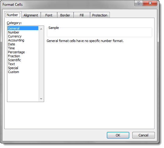
Underneath the pre-defined number formats for common items like currency and percentage, there is a category called Custom. The format types in this section are different from the pre-set options. They are filled with symbols and codes:
A number format code is entered into the Type field in the Custom category. These codes are the key to creating any custom number format in Excel. First, however, we need to understand how they work…
Understanding the Number Format Codes
Number format codes are the string of symbols that define how Excel displays the data you store in cells. We will get into the ways to describe the formats in a minute, but first we need to go over how Excel interprets those symbols. Each number format code is made up of as many as 4 sections separated by a semi-colon (;).
These sections control formatting for one or more parts of the number line, including positive numbers, negative numbers, and zeros. They can also control formatting for sub-sets of these parts, like all numbers greater than 100 and text-based data. What each section controls depends on how many sections there are in the number format code. A full number format code will be entered as follows:
Section1;Section2;Section3;Section4
The behavior of different parts of the number line will be as follows:
As indicated above, when there is just one section provided, it describes the format for all numbers. With two, the first section describes the format of positive, zero, and text values, while the second section describes the format of negative values, etc.
You can choose to skip formatting for any of the middle sections by entering General instead of other format data. For example, if you only want to affect positive numbers and text, you can enter a number format code with this arrangement:
Section1;General;General;Section4
General strips all formatting from the data entered, so be careful how you use it. Negative numbers with the General format code will not display the minus sign in front of their number.
Important note: Using a single section number format code does not always have the same result as expanding the same rules to all sections. For example:
Section1
Is not the same as:
Section1;Section1;Section1;Section1
Look at the examples below to see examples of the difference…
Now that we understand what a number format code is, what can we do with it?
Changing Font Color with Number Format Codes
One of the simplest things you can do with number format codes is change the color of the font in the affected cells. The syntax for doing so is simple:
[Color Name]
Just choose the section that corresponds to the part of the number line you want to change color, and provide the color in brackets. The color options are as follows (the background is gray for contrast in the table, but backgrounds are not affected by the number format code):
As an example, we can provide a separate color code for each part of a number format code:
[Red]General;[Blue]General;[Magenta]General;[Cyan]General
The General message just tells Excel to represent the numbers as entered by the user. The output of this number format code looks like this:
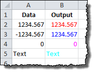
Note that the negative number in row 3 does not automatically get a negative sign (-) in front of it. We are overriding the default format of negative numbers in the cell. Also notice that the color format is not affecting anything about the presentation; the number of decimal places stays the same, as does the alignment of the data to the left or right of the cells.
Adding Text with Number Format Codes
You can add text around numbers with number format codes by inserting the text in a section one of two ways:
Single Characters
For single characters (like an @ symbol before a number), type a backslash () followed by the symbol. The number format code:
@General
Results in the following output:
Note that the minus sign still precedes the negative number. Also note that the Text value is not affected by the @ symbol addition.
Importantly, this is different from the result if we expanded our format guideline to each section of the number format code:
@General;@General;@General;@General
Results in the following output:
Note that the minus sign is gone from the negative number and the Text value now receives the @ symbol.
Text Strings
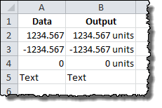
To add an entire text string to a number (like adding “units” to the end of a number), we surround the text string in quotation marks (” “). The number format code:
General" units"
Results in the following output:
Once again, this is different from:
General" units";General" units";General" units";General" units"
Which results in:

Special Characters
In addition to these two methods, there is a set of special symbol characters that do not need a leading backslash or quotes to be included in the number format code. The list is as follows:
Excel will also accept most other non-mathematical symbols, such a non-dollar currency symbols, copyright/trademark symbols, and Greek letters. These symbols are not available on most standard keyboards, but they can be entered by holding down the ALT key while typing in a four-digit number. Some of the most useful ones are below:
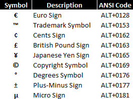
A full list of ANSI character codes can be found on Wikipedia here.
Changing Decimal Places, Significant Digits, and Commas
Adding symbols and colors is useful, but most of the work you’ll likely need to do with custom number formats is change the way Excel displays the numbers it stores. Number format codes use a set of symbols to represent how the data should appear in the cell. Here is a summary of the symbols:
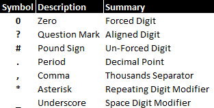
Let’s review them each in turn…
Zero (0)
Zeros in the number format code represent a forced digit. That means that whether or not the digit is relevant to the value, it will be shown. A great example of this is the standard dollars and cents notation that is used to represent prices in the United States: $0.00. Even if there are no extra cents in the amount, the two zeroes are still shown in the notation.
Here is an example of the zero code in action. The following examples are using this number format code:
0.00
Question Mark (?)
Question marks in the number format code represent an alignment digit. This means that when the number being shown doesn’t need the digit in question, a blank space of the same size is used. This is used to align decimal and comma places for more easy ranking of values, etc.
Here is an example of the question mark code in action. The following examples are using this number format code:
0.??
Pound Sign (#)
Sometimes called a hash mark, the pound sign in the number format code represents an optional digit. This means that when the number being shown doesn’t need the digit in question, it will be omitted from the displayed number. This is most often used to represent numbers in their most easily readable form.
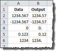
Here is an example of the pound sign code in action. The following examples are using this number format code:
#.##
Period (.)
The period in the number format code represents the location of the decimal point in the number being displayed. When paired with the comma code, it can show numbers in thousands or millions, changing 1,200 to 1.2, for example. It is similar to the text format codes above in that it is always displayed when it is part of the number code, even when number being displayed does not straddle the decimal point. See the comma, pound sign and question mark examples above for useful illustrations of the period in use.
Comma (,)
The comma in the number format code represents the thousands separators in the number being displayed. It allows you to describe the behavior of digits in relation to the thousands or millions digits.
Here is an example of the comma code in action. The following examples are using this number format code:
$??,???.00
Asterisk (*)
The asterisk in the number format code represents the repeating character modifier. It is used along with a character to display a repeating digit that fills the empty space in a cell.
Here is an example of the asterisk code in action. The following examples are using this number format code:
*=0.##
Underscore (_)
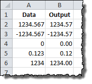
The underscore in the number code represents the space character modifier. It is used along with a character to display a blank space equal in size to the specified character. It can be used, for example, to properly align positive and negative numbers when parentheses are used in only the negative case.
Here is an example of the underscore code in action. The following examples are using this number format code:
_(#.##_);(#.##)
Using Fractions, Percentages, and Scientific Notation
Certain types of notation require that symbols be used to indicate the format change, including fractions, percentages, and scientific notation. Here is a summary of the symbols for each:
We’ll examine each in detail…
Fractions (/)
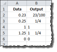
Fractions are special, since they require a change in units. The number 0.23 is represented as 23/100, but 0.25 can be simplified t0 1/4 or shown as 25/100. Similarly, 1.25 can be shown as 1 1/4 or the improper fraction 5/4. Which way Excel displays the number depends on how you construct the number format code.
Fractions effectively round values to the nearest possible fraction. They also take the guidelines of the pound sign and question mark symbols they are paired with.
Integer with Reduced Fractions
A fairly typical representation for fractions is to keep the whole numbers independent from the fraction remainder. The representation for this is relatively straightforward and can be done with pound signs and question marks to slightly different effect…
Using question mark (?) notation, the following number format code:
# ???/???
Produces a fraction remainder with up to three digits:
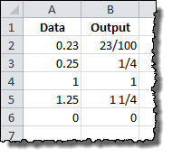
The alignment of the fraction bar is preserved regardless of the number of digits in use. If we limit the number of digits on each side of the fraction to 2, Excel will round the number to the nearest fraction value. The following number code format:
# ??/??
Changes the representation of 0.23 from 23/100 to 3/13.
If you don’t wish to preserve the alignment around the fraction bar, you can use a similar fraction number format code that uses pound signs.
Using pound sign notation, the following number format code:
# ###/###
Produces a more readable fraction remainder that can be justified or centered in the cell:
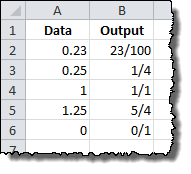
Improper Fractions
If you’d rather bundle the whole number portion of a value into the fraction itself, you can specify as much in the number format code.
Using pound sign notation, the following number format code:
###/###
Produces an improper fraction with up to three digits:
Fixed Base Fractions
It is also possible to force Excel to round fractions to a specific denominator by specifying it in the number format code.
Here is an example of a fixed base code in action. The following examples are using this number format code:
# ##/15
The result is a rounded fraction remainder that goes to the nearest number of 15ths.
Percentages (%)
Much like fractions, percentages are controlled by the number format codes that accompany them. A basic percentage can be achieved with a pound sign symbol in the number format code:
#%
Results in the following output:
You can also specify fractional percentages, as shown with this number format code:
# #/#%
Results in single-digit fractions in the percentages where needed:
Finally, as always, you can specify the number of significant digits with decimal places:
#.0%
Results in a 10th place aligned decimal:
Scientific Notation (E)
It’s difficult to read extremely small and extremely large numbers conventionally because of all the leading and trailing zeroes. Scientific notation fixes that by moving the decimal to the relevant digits, so 0.0000001 can become 1 x 10⁻⁷. Excel uses the E notation for this, so that same number would be 1E-07. So, as you’d expect, the capital letter E signals scientific notation in number format code.
Otherwise, scientific notation in Excel is controlled by the same number codes as percentages and fractions. It needs a number format code in front of the E to describe the relevant digits and a plus (+) and another number format code behind to describe the handling of the exponential digit.
Here is an example of a scientific notation code in action. The following examples are using this number format code:
#E+#
You can also achieve more consistent notation with zeros. The following examples are using this number format code:
0.00E+00
Note that in this case, the decimal and exponent are both constrained to 2 significant digits, regardless of whether they are necessary. The trade-off is, it keeps the output far more consistent, with a predictable string length.
Dates and Times
Dates and times in Excel are a special case. For a detailed discussion of how Excel uses them, please review the Definitive Guide to Using Dates and Times in Excel. The number format codes work identically to the format_text input for the TEXT command, and they can be reviewed here.
Get the latest Excel tips and tricks by joining the newsletter!
 Andrew Roberts has been solving business problems with Microsoft Excel for over a decade. Excel Tactics is dedicated to helping you master it.
Join the newsletter to stay on top of the latest articles. Sign up and you’ll get a free guide with 10 time-saving keyboard shortcuts!
Other posts in this series…
Introduction
Number formats control how numbers are displayed in Excel. The key benefit of number formats is that they change how a number looks without changing any data. They are a great way to save time in Excel because they perform a huge amount of formatting automatically. As a bonus, they make worksheets look more consistent and professional.
Video: What is a number format
What can you do with custom number formats?
Custom number formats can control the display of numbers, dates, times, fractions, percentages, and other numeric values. Using custom formats, you can do things like format dates to show month names only, format large numbers in millions or thousands, and display negative numbers in red.

Where can you use custom number formats?
Many areas in Excel support number formats. You can use them in tables, charts, pivot tables, formulas, and directly on the worksheet.
- Worksheet — format cells dialog
- Pivot Tables — via value field settings
- Charts — data labels and axis options
- Formulas — via the TEXT function
What is a number format?
A number format is a special code to control how a value is displayed in Excel. For example, the table below shows 7 different number formats applied to the same date, January 1, 2019:
| Input | Code | Result |
|---|---|---|
| 1-Jan-2019 | yyyy | 2019 |
| 1-Jan-2019 | yy | 19 |
| 1-Jan-2019 | mmm | Jan |
| 1-Jan-2019 | mmmm | January |
| 1-Jan-2019 | d | 1 |
| 1-Jan-2019 | ddd | Tue |
| 1-Jan-2019 | dddd | Tuesday |
The key thing to understand is that number formats change the way numeric values are displayed, but they do not change the actual values.
Where can you find number formats?
On the home tab of the ribbon, you’ll find a menu of build-in number formats. Below this menu to the right, there is a small button to access all number formats, including custom formats:

This button opens the Format Cells dialog box. You’ll find a complete list of number formats, organized by category, on the Number tab:

Note: you can open Format Cells dialog box with the keyboard shortcut Control + 1.
General is default
By default, cells start with the General format applied. The display of numbers using the General number format is somewhat «fluid». Excel will display as many decimal places as space allows, and will round decimals and use scientific number format when space is limited. The screen below shows the same values in column B and D, but D is narrower and Excel makes adjustments on the fly.

How to change number formats
You can select standard number formats (General, Number, Currency, Accounting, Short Date, Long Date, Time, Percentage, Fraction, Scientific, Text) on the home tab of the ribbon using the Number Format menu.
Note: As you enter data, Excel will sometimes change number formats automatically. For example if you enter a valid date, Excel will change to «Date» format. If you enter a percentage like 5%, Excel will change to Percentage, and so on.
Shortcuts for number formats
Excel provides a number of keyboard shortcuts for some common formats:
| Format | Shortcut |
|---|---|
| General format | Ctrl Shift ~ |
| Currency format | Ctrl Shift $ |
| Percentage format | Ctrl Shift % |
| Scientific format | Ctrl Shift ^ |
| Date format | Ctrl Shift # |
| Time format | Ctrl Shift @ |
| Custom formats | Control + 1 |
See also: 222 Excel Shortcuts for Windows and Mac
Where to enter custom formats
At the bottom of the predefined formats, you’ll see a category called custom. The Custom category shows a list of codes you can use for custom number formats, along with an input area to enter codes manually in various combinations.

When you select a code from the list, you’ll see it appear in the Type input box. Here you can modify existing custom code, or to enter your own codes from scratch. Excel will show a small preview of the code applied to the first selected value above the input area.
Note: Custom number formats live in a workbook, not in Excel generally. If you copy a value formatted with a custom format from one workbook to another, the custom number format will be transferred into the workbook along with the value.
How to create a custom number format
To create custom number format follow this simple 4-step process:
- Select cell(s) with values you want to format
- Control + 1 > Numbers > Custom
- Enter codes and watch preview area to see result
- Press OK to save and apply
Tip: if you want base your custom format on an existing format, first apply the base format, then click the «Custom» category and edit codes as you like.
How to edit a custom number format
You can’t really edit a custom number format per se. When you change an existing custom number format, a new format is created and will appear in the list in the Custom category. You can use the Delete button to delete custom formats you no longer need.
Warning: there is no «undo» after deleting a custom number format!
Structure and Reference
Excel custom number formats have a specific structure. Each number format can have up to four sections, separated with semi-colons as follows:

This structure can make custom number formats look overwhelmingly complex. To read a custom number format, learn to spot the semi-colons and mentally parse the code into these sections:
- Positive values
- Negative values
- Zero values
- Text values
Not all sections required
Although a number format can include up to four sections, only one section is required. By default, the first section applies to positive numbers, the second section applies to negative numbers, the third section applies to zero values, and the fourth section applies to text.
- When only one format is provided, Excel will use that format for all values.
- If you provide a number format with just two sections, the first section is used for positive numbers and zeros, and the second section is used for negative numbers.
- To skip a section, include a semi-colon in the proper location, but don’t specify a format code.
Characters that display natively
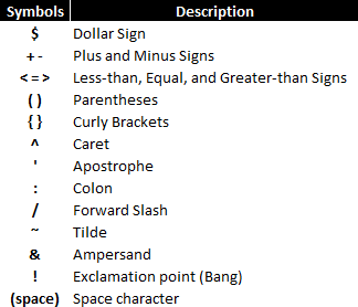
Some characters appear normally in a number format, while others require special handling. The following characters can be used without any special handling:
| Character | Comment |
|---|---|
| $ | Dollar |
| +- | Plus, minus |
| () | Parentheses |
| {} | Curly braces |
| <> | Less than, greater than |
| = | Equal |
| : | Colon |
| ^ | Caret |
| ‘ | Apostrophe |
| / | Forward slash |
| ! | Exclamation point |
| & | Ampersand |
| ~ | Tilde |
| Space character |
Escaping characters
Some characters won’t work correctly in a custom number format without being escaped. For example, the asterisk (*), hash (#), and percent (%) characters can’t be used directly in a custom number format – they won’t appear in the result. The escape character in custom number formats is the backslash (). By placing the backslash before the character, you can use them in custom number formats:
| Value | Code | Result |
|---|---|---|
| 100 | #0 | #100 |
| 100 | *0 | *100 |
| 100 | %0 | %100 |
Placeholders
Certain characters have special meaning in custom number format codes. The following characters are key building blocks:
| Character | Purpose |
|---|---|
| 0 | Display insignificant zeros |
| # | Display significant digits |
| ? | Display aligned decimals |
| . | Decimal point |
| , | Thousands separator |
| * | Repeat following character |
| _ | Add space |
| @ | Placeholder for text |
Zero (0) is used to force the display of insignificant zeros when a number has fewer digits than zeros in the format. For example, the custom format 0.00 will display zero as 0.00, 1.1 as 1.10 and .5 as 0.50.

Pound sign (#) is a placeholder for optional digits. When a number has fewer digits than # symbols in the format, nothing will be displayed. For example, the custom format #.## will display 1.15 as 1.15 and 1.1 as 1.1.

Question mark (?) is used to align digits. When a question mark occupies a place not needed in a number, a space will be added to maintain visual alignment.

Period (.) is a placeholder for the decimal point in a number. When a period is used in a custom number format, it will always be displayed, regardless of whether the number contains decimal values.
Comma (,) is a placeholder for the thousands separators in the number being displayed. It can be used to define the behavior of digits in relation to the thousands or millions digits.

Asterisk (*) is used to repeat characters. The character immediately following an asterisk will be repeated to fill remaining space in a cell.

Underscore (_) is used to add space in a number format. The character immediately following an underscore character controls how much space to add. A common use of the underscore character is to add space to align positive and negative values when a number format is adding parentheses to negative numbers only. For example, the number format «0_);(0)» is adding a bit of space to the right of positive numbers so that they stay aligned with negative numbers, which are enclosed in parentheses.

At (@) — placeholder for text. For example, the following number format will display text values in blue:
0;0;0;[Blue]@
See below for more information about using color.
Automatic rounding
It’s important to understand that Excel will perform «visual rounding» with all custom number formats. When a number has more digits than placeholders on the right side of the decimal point, the number is rounded to the number of placeholders. When a number has more digits than placeholders on the left side of the decimal point, extra digits are displayed. This is a visual effect only; actual values are not modified.
Number formats for TEXT
To display both text along with numbers, enclose the text in double quotes («»). You can use this approach to append or prepend text strings in a custom number format, as shown in the table below.
| Value | Code | Result |
|---|---|---|
| 10 | General» units» | 10 units |
| 10 | 0.0″ units» | 10.0 units |
| 5.5 | 0.0″ feet» | 5.5 feet |
| 30000 | 0″ feet» | 30000 feet |
| 95.2 | «Score: «0.0 | Score: 95.2 |
| 1-Jun | «Date: «mmmm d | Date: June 1 |
Number formats for DATES
Dates in Excel are just numbers, so you can use custom number formats to change the way they display. Excel has many specific codes you can use to display components of a date in different ways. The screen below shows how Excel displays the date in D5, September 3, 2018, with a variety of custom number formats:

Number formats for TIME
Times in Excel are fractional parts of a day. For example, 12:00 PM is 0.5, and 6:00 PM is 0.75. You can use the following codes in custom time formats to display components of a time in different ways. The screen below shows how Excel displays the time in D5, 9:35:07 AM, with a variety of custom number formats:

Note: m and mm can’t be used alone in a custom number format since they conflict with the month number code in date format codes.
Number formats for ELAPSED TIME
Elapsed time is a special case and needs special handling. By using square brackets, Excel provides a special way to display elapsed hours, minutes, and seconds. The following screen shows how Excel displays elapsed time based on the value in D5, which represents 1.25 days:

Number formats for COLORS
Excel provides basic support for colors in custom number formats. The following 8 colors can be specified by name in a number format: [black] [white] [red][green] [blue] [yellow] [magenta] [cyan]. Color names must appear in brackets.

Colors by index
In addition to color names, it’s also possible to specify colors by an index number (Color1,Color2,Color3, etc.) The examples below are using the custom number format: [ColorX]0″▲▼», where X is a number between 1-56:
[Color1]0"▲▼" // black
[Color2]0"▲▼" // white
[Color3]0"▲▼" // red
[Color4]0"▲▼" // green
etc.
The triangle symbols have been added only to make the colors easier to see. The first image shows all 56 colors on a standard white background. The second image shows the same colors on a gray background. Note the first 8 colors shown correspond to the named color list above.


Apply number formats in a formula
Although most number formats are applied directly to cells in a worksheet, you can also apply number formats inside a formula with the TEXT function. For example, with a valid date in A1, the following formula will display the month name only:
=TEXT(A1,"mmmm")
The result of the TEXT function is always text, so you are free to concatenate the result of TEXT to other strings:
="The contract expires in "&TEXT(A1,"mmmm")
The screen below shows the number formats in column C being applied to numbers in column B using the TEXT function:

One quirk of the TEXT function relates to double quotes («») that are part of certain custom number formats. Because the format_text is entered as a text string, Excel won’t allow you to enter the formula without removing the quotes or adding more quotes. For example, to display a large number in thousands, you can use a custom number format like this:
0, "k"Notice k appears in quotes («k»). To apply the same format with the TEXT function, you can use simply:
=TEXT(A1,"0, k")Notice the k is not surrounded by quotes. Alternately, you can add extra double quotes as below, which returns the same result:
=TEXT(A1,"0,""K""")This behavior only occurs when you are hardcoding a format inside TEXT. If you are applying a format entered elsewhere on the worksheet (as in cells C6 and C9 in the worksheet above) you can use a standard number format.
Measurements
You can use a custom number format to display numbers with an inches mark («) or a feet mark (‘). In the screen below, the number formats used for inches and feet are:
0.00 ' // feet
0.00 " // inches

These results are simplistic, and can’t be combined in a single number format. You can however use a formula to display feet together with inches.
Conditionals
Custom number formats also up to two conditions, which are written in square brackets like [>100] or [<=100]. When you use conditionals in custom number formats, you override the standard [positive];[negative];[zero];[text] structure. For example, to display values below 100 in red, you can use:
[Red][<100]0;0
To display values greater than or equal to 100 in blue, you can extend the format like this:
[Red][<100]0;[Blue][>=100]0

To apply more than two conditions, or to change other cell attributes, like fill color, etc. you’ll need to switch to Conditional Formatting, which can apply formatting with much more power and flexibility using formulas.
Plural text labels
You can use conditionals to add an «s» to labels greater than zero with a custom format like this:
[=1]0″ day»;0″ days»

Telephone numbers
Custom number formats can also be used for telephone numbers, as shown in the screen below:

Notice the third and fourth examples use a conditional format to check for numbers that contain an area code. If you have data that contains phone numbers with hard-coded punctuation (parentheses, hyphens, etc.) you will need to clean the telephone numbers first so that they only contain numbers.
Hide all content
You can actually use a custom number format to hide all content in a cell. The code is simply three semi-colons and nothing else ;;;
To reveal the content again, you can use the keyboard shortcut Control + Shift + ~, which applies the General format.
Other resources
- Developer Bryan Braun built a nice interactive tool for building custom number formats
Excel Numbering (Table of Contents)
- Numbering in Excel
- How to Add Serial Number in Excel?
Numbering in Excel
There are various ways of numbering in excel, which are Fill Handle, Fill Series, Row Function mainly. By Fill Handle, we can drag already written 2-3 numbers in sequence until the limit we want. By Fill Series, which is available in the Home menu tab and select the Series option, select the lowest and highest numbers. And if we select the Row function for numbering, then also we can create a number in the sequence.
How to Add Serial Number in Excel?
To add a serial number in Excel is very simple and easy. Let’s understand the working of adding a serial number in Excel by some methods with its example.
You can download this Numbering Excel Template here – Numbering Excel Template
Example #1 – Fill Handle Method
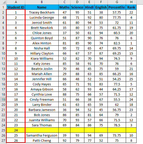
Suppose you have the following dataset. And you have to give a Student ID to each entry. Student ID there will be the same as a serial number of each row entry.
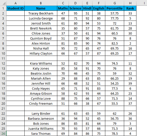
You can use the fill handle method here.
For example, you want to give Student ID 1056 to the first student, and after it should be numerically increasing, 1056, 1057,1058, and so on…
Steps to number rows in Excel:
- Enter 1056 in cell A2 and 1057 in cell A3.
- Select both cells.
- Now you can notice a square at the bottom-right of selected cells.
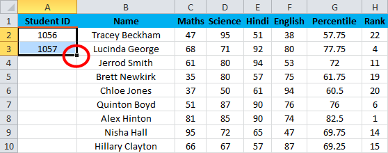
- Move your cursor to this square; now, it will be changed to the small plus sign.
- Now double click this plus icon, and it will automatically fill the series till the end of the dataset.
Key Point:
- It identifies a pattern from a few filled cells and quickly fills the entire selected column.
- It would only work till the last contiguous non-blank row. Viz. If you have any blank row(s) between your dataset. It will not detect them, so it’s not recommended to use the fill method.
Example #2 – Fill Series Method
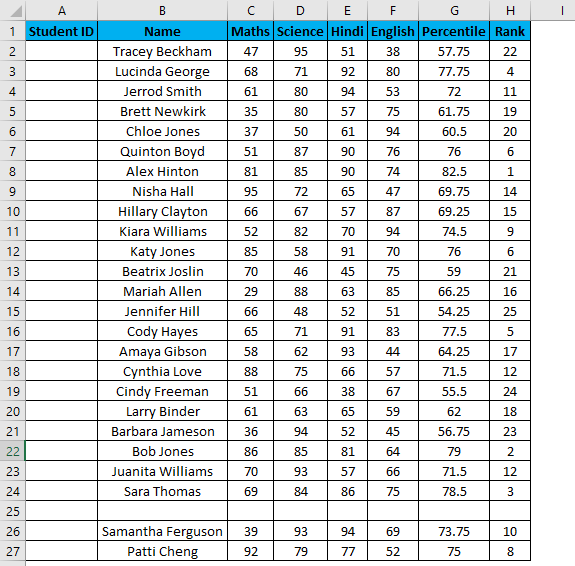
Suppose now we have the following dataset (same as above, now entries are only 26.).
Steps to use the Fill Series method:
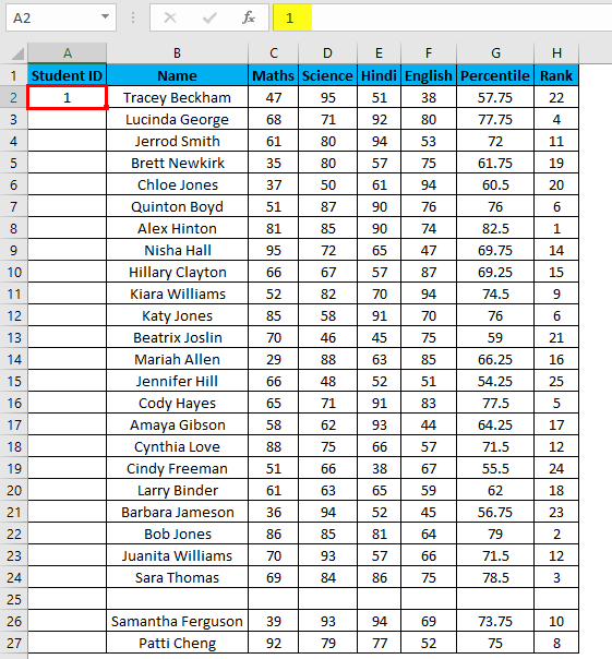
- Enter 1 in cell A2.
- Go to the Home tab.
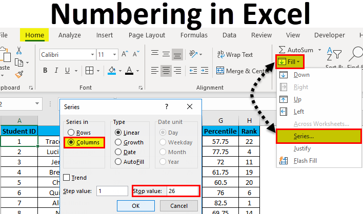
- In the Editing group, click on the Fill drop-down.
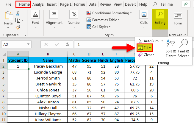
- From the drop-down, select Series.
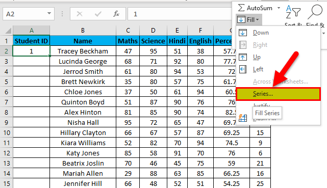
- In the Series dialog box, select Columns in the ” Series in ” option.
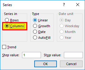
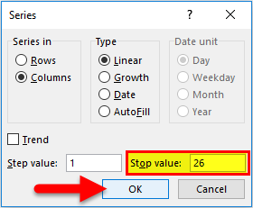
- Specify the Stop value. Here we can enter 26 and then click Ok.
- If you don’t enter any value, Fill Series will not work.
Hotkey to use fill series: ALT key+ H+ FI+ S
You can notice, it overcomes the drawback of the previous method. But then it has its own drawback that if we have blank rows in between of the dataset, Fill Series would still fill the number for that row.
Example #3 – COUNTA Function
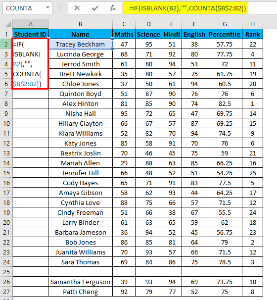
Suppose you have the same data set as above, now if you want to number rows in excel only which are filled Viz. Overcoming the shortcomings of the above 2 methods. You can use a COUNTA function here.
Steps to use a COUNTA Function:
- Now enter the formula in the cell A2 i.e. =IF(ISBLANK(B2),””,COUNTA($B$2:B2))
- Drag it down till the last row of your data set.
- In the above formula, the IF function will check if cell B2 is empty or not. If found empty, it returns a blank, but it returns the count of all the filled cells till that cell if it’s not.
Example #4 – Increment Previous Row Number
This is a very simple method. The main method is to add 1 to the previous row number simply.
Suppose you again have the same dataset.
- In the first row, manually enter 1 or any number from where you want to start numbering all rows in excel. In our case. Enter 1 in cell A2.
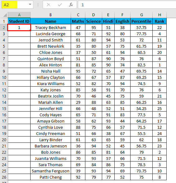
- Now in cell A3, simply enter the formula=A2+1.
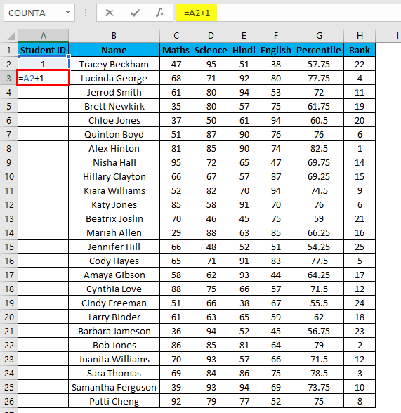
- Drag this formula until the last row, and it will be increased by 1 in each following row.
Example #5 – Row Function
We can even use a row function to give serial numbers to rows in our columns. In above all methods, the serial number inserted is fixed values. But what if a row is moved or you cut and paste data somewhere else in the worksheet?
The above problem can be resolved by using the ROW function. To number the rows in a given dataset using the ROW function.
- Enter the formula in the first cell i.e. =IF(ISBLANK(B2),””,ROW()-1)
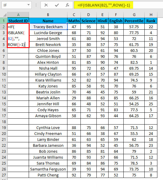
- Drag this formula until the last row.
- In the above formula IF function will check if the adjacent cell B is blank or not. If it’s found blank, it will return space, and if non-blank, then row function will come into the picture. ROW() function will give us the row number since the first row in Excel consists of our dataset. So we don’t need to count it. To eliminate the first row, I have subtracted 1 from the returned value of the above function.
- But it will not still adjust the row number, and a blank row will still have a serial number assigned to it. Though it is not shown, look at the below screenshot.
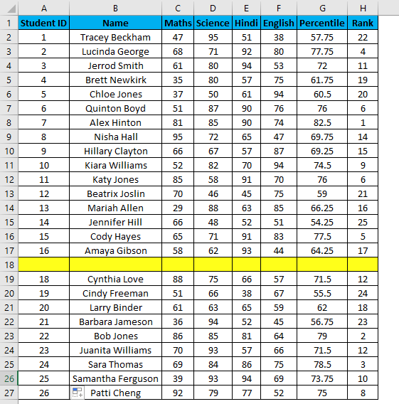
- You can overcome the above issue with this formula, i.e.=ROW()-1
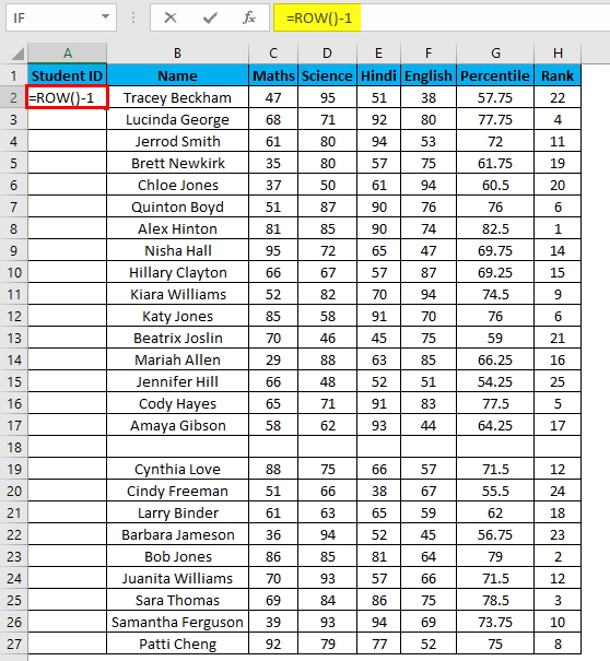
- Drag this formula until the last row.
- But now, it will consider the blank rows in the dataset and will number them as well. Consider the below screenshot.
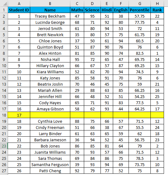
The main advantage of using this method is even if you delete one or more entries in your dataset. You don’t need to struggle with the numbering of rows each and every time, and it will be corrected automatically in excel.
So by now, I have discussed 5 unique methods to give serial numbers to row in a dataset stored in Excel. Although there are numerous methods to do the same, above five are the most common and easy to use method which can be implemented in different scenarios.
Things to Remember About Numbering in Excel
- While storing data in Excel, we often need to give serial numbers to each row in our data set.
- Entering a serial number to each and every row in the huge dataset can be time-consuming and prone to error.
Recommended Articles
This has been a guide to Numbering in Excel. Here we discuss how to add serial Numbers using different methods in excel along with practical examples and a downloadable excel template. You can also go through our other suggested articles –
- ISNUMBER Excel Function
- Negative Numbers in Excel
- Excel ISNUMBER Formula
- VBA Number Format
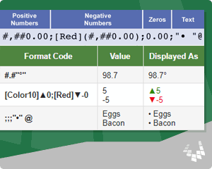
In Excel, you aren’t limited to using built-in number formats. You can define your own custom number formats to display values as thousands or millions (23K or 95.3M), add leading zeros, display » — » for zero values, make negative values red, add bullets, and much more.
This Article (bookmarks):
- Watch the Video Overview
- How to Create a Custom Number Format
- Number Format Codes
- Examples
- Format for Thousands and Millions
- Display Leading Zeros and Include Commas
- Display Units Without Converting to Text
- Special Time Formats
- Including Special Symbols
- Displaying Fractions
- Trailing and Leading Characters to Fill a Cell
- Chart Axes and Labels
- Using Color Codes
- Conditional Operators
- Custom Location Codes for Dates
Watch the video we created to go along with this article!
How to Create a Custom Number Format
To create a custom number format, it is easiest to begin with a built-in format. Open the Format Cells dialog box by pressing Ctrl+1 (or right-click on a cell and select Format Cells) and select the Number tab (see the image below). Then (1) Choose Custom from the Category list, (2) Select a built-in format similar to what you want, and (3) Edit the format string in the Type field.
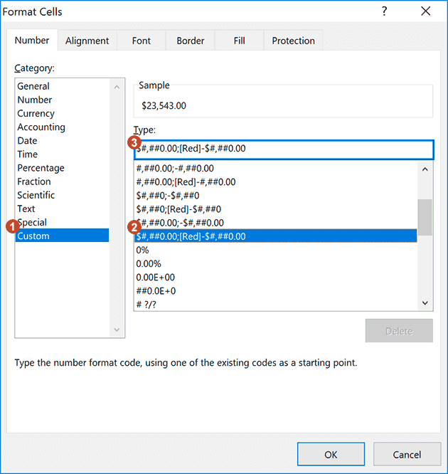
Number Format Codes
A number format string uses up to 4 different codes, separated by semicolons, as shown in the image below.
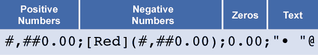
Instead of explaining the syntax in detail at this point, let’s take a look at some examples and learn as we go.
Some of the characters like #, 0, @, etc. have special meanings. Some codes like [Red] can change the font color, and quotes can be used to display text or special characters. The table below summarizes some of these special characters.
Special Characters in Number Formats
| Character | Description |
|---|---|
| # | A digit placeholder |
| 0 | A digit that is to be displayed even if it is zero |
| , | (Comma) Interpreted as a 1000’s marker |
| @ | Represents the value displayed as text |
| * | (Asterisk) Repeats the next character to fill the cell |
| [ColorCode] | See the section below about using color codes |
| [<=100] | Conditional operators (valid only in the Positive and Negative sections) |
| / | Used for fractions such as # #/12 or as the / character for dates |
| » « | (Quotes) Used to display whatever is contained within the quotes as text, such as 0.00 «feet» |
| d or dd ddd dddd |
Day number (0-31 or 00-31) Abbreviated day of week (Mon, Tue, etc.) Full day of week (Monday, Tuesday, etc.) |
| m or mm mmm mmmm mmmmm |
Month number (0-12 or 00-12) Abbreviated month name (Jan, Feb, etc.) Full month name (January, February, etc.) First letter of the month (J, F, M, etc.) |
| y or yy yyyy |
Year (0-99 or 00-99) Full year (1900-9999) |
| h or hh m or mm s or ss |
Hour (0-23 or 00-23) Minutes (0-59 or 00-59) Seconds (0-59 or 00-59) |
NOTE Some characters are specific to locale/language settings. For example J is used for Year in some countries.
Custom Number Format Examples
The examples below show some of the custom number formats that I’ve found the most useful. This isn’t a comprehensive list of all possible number formats. See support.microsoft.com to search for other articles on this subject.
TIP Using a custom number format only affects the displayed value. A formula that references the cell will use the stored value no matter how it is displayed. This means you can still use a formula to refer to the value even though the number might be displayed as «12 ft.»
To see these examples in action, download the Excel file below.
Download the Example File (CustomNumberFormats.xlsx)
Custom Number Format for Thousands and Millions
| Format Code | Value | Displayed As | Description |
|---|---|---|---|
| 0,K 0.0,K 0.0, «Thousand» |
23543 | 24K 23.5K 23.5 Thousand |
Display values in thousands, using the letter K to indicate thousands. The «K» is just a displayed character — it has no special meaning in the number format string. If you want to display more than one letter, you need to enclose the characters in quotes, like the «Thousand» example. |
| 0,,»M» 0.0,,»M» 0.0,, «Million» |
23543000 | 24M 23.5M 23.5 Million |
Display values in millons, using the letter M to indicate millions. Note that in this case, you need two commas. |
NOTE These are very useful for chart axes and labels.
Display Leading Zeros and Include Commas
| Format Code | Value | Displayed As | Description |
|---|---|---|---|
| 000 00000 |
50.8 | 051 00051 |
Display values with leading zeros. This does not convert the value to text — it is only a display format. |
| #,##0.0 | 3543.46 | 3,543.5 | Display values using commas to separate thousands, millions, etc. The # sign is used as a placeholder, meaning that if there are no 10’s, 100’s, or 1000’s, don’t display them. |
Display Units Without Converting to Text
| Format Code | Value | Displayed As |
|---|---|---|
| • Display a number and text in the same cell using the conditions [=1] and [>1]. The value is stored as a number, so you can still do calculations on the number of people. | ||
| [=1]# «person»;[>1]# «people»;0 | 1 5 0 |
1 person 5 people 0 |
| • Display a number and text in the same cell. The value is stored as a number, so you can still do calculations. | ||
| 0.0 «ft» 0.0 «kg» # #/## «in» |
2.2 4.5 6.25 |
2.2 ft 4.5 kg 6 1/4 in |
| • Display a numeric YYMMDD value in years, months, days. | ||
| ##»y» ##»m» ##»d» | 360712 | 36y 07m 12d |
Special Time Formats
There are quite a few built-in time formats to choose from. The following may be less known.
| Format Code | Value | Displayed As | Description |
|---|---|---|---|
| [h]:mm:ss [h]:mm [mm]:ss [ss] |
49:03:47 | 49:03:47 49:03 2943:47 176627 |
Shows elapsed time in hours, minutes or seconds. Note that time does not round up. |
| h:mm A/P h:mm a/p |
2:25 PM | 2:25 P 2:25 p |
Displays time using «a» for AM and «p» for PM. Useful when trying to minimize column widths without making fonts smaller. |
Including Special Symbols
Some ascii and unicode characters can be copied and pasted directly into the format code. This can be handy for displaying the degrees symbol for temperatures as well as other tricks like showing up and down arrows or bulleted lists.
| Format Code | Value | Displayed As | Description |
|---|---|---|---|
| #.#»°» | 98.7 | 98.7° | Display temperature in degrees with the ° symbol. |
| [Color10]▲0;[Red]▼-0 | 5 -5 |
▲5 ▼-5 |
Display special symbols for positive and negative, combined with colors. |
| ;;;»•» @ | Eggs Bacon |
• Eggs • Bacon |
Create a bulleted list using a special symbol for the bullet. When you enter text, the bullet will be displayed. Numbers and zero values will not be displayed. |
Displaying Fractions
| Format Code | Value | Displayed As | Description |
|---|---|---|---|
| # ??/12 | 5.75 12.5 |
5 9/12 12 6/12 |
Display a decimal number of feet as feet and inches (rounded to the nearest inch). Or display a decimal year in terms of years and months. |
| # ??/100 | 5.2 5.05 12.81 |
5 20/100 5 5/100 12 81/100 |
Using ??/100 will help line up values in a column (as opposed to just using ?/100). Note that fractions are automatically rounded. |
| ?/2 | 5.2 | 10/2 | Displays a simple fraction as numerator/denominator. |
Trailing and Leading Characters to Fill a Cell
The asterisk (*) in a format code repeats the following character to fill the width of the cell.
| Format Code | Value | Displayed As | Description |
|---|---|---|---|
| — @ *- | ✁ | — ✁ —————- | Trailing characters. |
| *.@ | pg 2 | ………………pg 2 | Leading characters |
Custom Number Formats for Chart Axes and Labels
| Format Code | Value | Displayed As | Description |
|---|---|---|---|
| 0 «AD»;0 «BC» | 247 -600 |
247 AD 600 BC |
AD and BC Years. Use negative numbers for BC years and positive numbers for AD years. |
| mmm{Ctrl+j}yyyy | 8/20/18 | Aug 2018 |
Add a Carriage Return within the custom number format (e.g. between dddd and mmm) by pressing Ctrl+j. |
| [Color10]▲0.0%;[Red]▼-0.0% | 15.23% -23.57% |
▲15.2% ▼-23.6% |
Display arrows for positive and negative, combined with colors and percentages. |
A couple of these examples can be seen in the image below. However, notice that the data labels don’t use color codes, so the percentages are shown only as black text rather than red and green. Too bad. Maybe Microsoft will fix that some day.
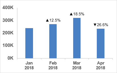
NOTE Editing a custom number format that contains a carriage return is tricky because you can’t see the second row. This is why I write out the code first using «{Ctrl+j}» or just «{j}» and then delete the «{j}» and press Ctrl+j in its place.
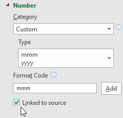
When adding a custom number format using the Format Axis window pane, you may not be able to press Ctrl+j to add a carriage return. In that case, first edit the format of the data source, then click on the Link to Source box as shown in the image to the right. After doing that, you can uncheck the Link to Source box and modify the original data source formatting.
Other Tricks
| Format Code | Value | Displayed As | Description |
|---|---|---|---|
| ;;; | anything | Display nothing, regardless of the value. | |
| 0.# | 2 | 2. | Display a decimal point without a 0 after the decimal (2. instead of 2.0) |
| ???.??? | 1.2 12.3 123.456 |
1.2 12.3 123.456 |
Vertically align the decimal point when displaying a column of numbers. |
NOTE If you are looking for format codes for phone numbers, social security numbers, or zip codes, look in the Special category within the list of built-in number formats.
Custom Number Format Color Codes
By using color format codes such as [Red] or [Blue] or [Color10], you have a limited ability to alter the color of the font via custom number formats. The most common use I’ve seen is to color negative values red. However, one of the examples above also shows how you might want to use a green arrow.
Even though a new color palette was introduced in Excel 2007, the color codes for custom number formats are still based on the old color palette for the Excel 97-2003 format. I created the graphic below to provide a quick reference.

I made the above color code reference match the layout of the old color palette because there is not a consistent pattern to the numbering.
Define Your Own Color: You can modify the color palette in newer versions of Excel by going to File > Options > Save > Colors. This allows you to change the color associated with the Color1 through Color56 codes. This means that Color10 might not always be a dark green. If you purposely change the color palette (or somebody else does), Color10 might be some other color.
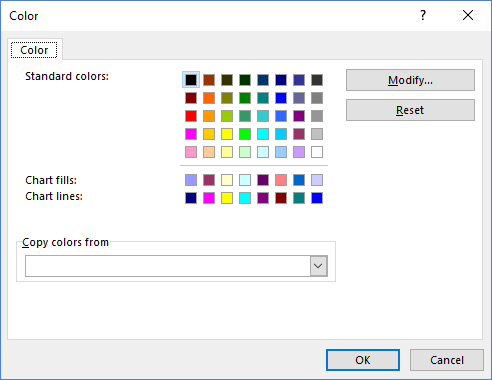
Excel 2016: File > Options > Save > Colors
NOTE The Color1-56 codes in Google Sheets are fixed colors and aren’t changed when you upload an Excel file with a customized color palette.
Conditional Operators
Conditional operators such as [<100] can be used to change the formatting in cases where positive;negative;0 is not how you want the divisions defined.
For example, the following format will display numbers less than 10 red, numbers between 10 and 20 green, other numbers blue, and text will be displayed based on the cell’s font color: [Red][<10]0.00;[Green][<=20]0.00;[Blue]0.00;@
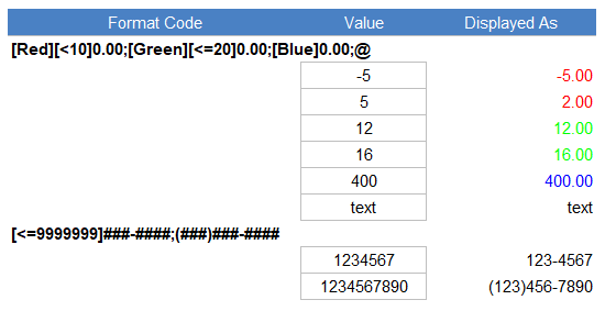
You are limited to 2 numeric conditions, which you place in the negative and positive sections of the format code.
Another use of conditional operators is to display phone numbers with and without an area code, depending on how many digits are in the phone number like this: [<=9999999]###-####;(###)###-####. This assumes that the phone numbers are entered as numbers and not text values. Meaning, that if you actually enter 123-1234 into a cell in Excel, it will be interpreted as a text value, not a number. The phone number format will display 1234567 to 123-4567 and it will display 1234567890 to (123)456-7890.
Custom Location Codes for Dates
When displaying month names and weekday names for dates, you can use location codes such as [$-fr-CA] at the beginning of the format code to tell Excel to display the names in other languages. To learn what the code is for a specific language and location, use the Format Cells dialog in Excel, choose one of the built-in Date formats, then choose the Locale (location) from the drop-down list. Then you can return to the Format Cells dialog box and click on the Custom tab to see what location code was added.
| Format Code | Value | Displayed As | Language/Location |
|---|---|---|---|
| [$-en-US](ddd) mmm d, yyyy | 10/1/2018 | (Mon) Oct 1, 2018 | English (United States) |
| [$-fr-CA](ddd) mmm d, yyyy | 8/1/2018 | (mer.) août 1, 2018 | French (Canada) |
| [$-de-DE](ddd) mmm d, yyyy | 10/1/2018 | (Mo) Okt 1, 2018 | German (Germany) |
Other Notes About Custom Number Formats
To delete a custom number format, open the Format Cells dialog box, select the custom format from the list, then click Delete. When you delete a custom number format, all values in your workbook that use that format will revert to the General format.
Custom number formats that you create are saved with the file. If you want to use the custom format in a different file, you can copy/paste the formatting from your other file by copying and pasting the formatted cell or using the Format Painter tool.
References
- Number Formats for Charts by Jon Peltier, Excel MVP
- Excel Custom Number Format Guide by Mynda Treacy, Excel MVP