
Excel for Microsoft 365 Excel for Microsoft 365 for Mac Excel for the web Excel 2021 Excel 2021 for Mac Excel 2019 Excel 2019 for Mac Excel 2016 Excel 2016 for Mac Excel 2013 Excel 2010 Excel 2007 More…Less
Although Excel includes a multitude of built-in worksheet functions, chances are it doesn’t have a function for every type of calculation you perform. The designers of Excel couldn’t possibly anticipate every user’s calculation needs. Instead, Excel provides you with the ability to create custom functions, which are explained in this article.
Custom functions, like macros, use the Visual Basic for Applications (VBA) programming language. They differ from macros in two significant ways. First, they use Function procedures instead of Sub procedures. That is, they start with a Function statement instead of a Sub statement and end with End Function instead of End Sub. Second, they perform calculations instead of taking actions. Certain kinds of statements, such as statements that select and format ranges, are excluded from custom functions. In this article, you’ll learn how to create and use custom functions. To create functions and macros, you work with the Visual Basic Editor (VBE), which opens in a new window separate from Excel.
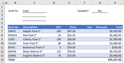
Suppose your company offers a quantity discount of 10 percent on the sale of a product, provided the order is for more than 100 units. In the following paragraphs, we’ll demonstrate a function to calculate this discount.
The example below shows an order form that lists each item, quantity, price, discount (if any), and the resulting extended price.
To create a custom DISCOUNT function in this workbook, follow these steps:
-
Press Alt+F11 to open the Visual Basic Editor (on the Mac, press FN+ALT+F11), and then click Insert > Module. A new module window appears on the right-hand side of the Visual Basic Editor.
-
Copy and paste the following code to the new module.
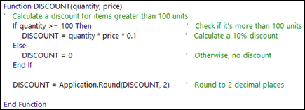
Function DISCOUNT(quantity, price)
   If quantity >=100 Then
     DISCOUNT = quantity * price * 0.1
   Else
     DISCOUNT = 0
   End If

 DISCOUNT = Application.Round(Discount, 2)
End Function
Note: To make your code more readable, you can use the Tab key to indent lines. The indentation is for your benefit only, and is optional, as the code will run with or without it. After you type an indented line, the Visual Basic Editor assumes your next line will be similarly indented. To move out (that is, to the left) one tab character, press Shift+Tab.
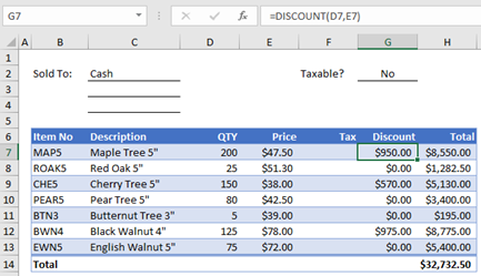
Now you’re ready to use the new DISCOUNT function. Close the Visual Basic Editor, select cell G7, and type the following:
=DISCOUNT(D7,E7)
Excel calculates the 10 percent discount on 200 units at $47.50 per unit and returns $950.00.
In the first line of your VBA code, Function DISCOUNT(quantity, price), you indicated that the DISCOUNT function requires two arguments, quantity and price. When you call the function in a worksheet cell, you must include those two arguments. In the formula =DISCOUNT(D7,E7), D7 is the quantity argument, and E7 is the price argument. Now you can copy the DISCOUNT formula to G8:G13 to get the results shown below.
Let’s consider how Excel interprets this function procedure. When you press Enter, Excel looks for the name DISCOUNT in the current workbook and finds that it is a custom function in a VBA module. The argument names enclosed in parentheses, quantity and price, are placeholders for the values on which the calculation of the discount is based.
The If statement in the following block of code examines the quantity argument and determines whether the number of items sold is greater than or equal to 100:
If quantity >= 100 Then
 DISCOUNT = quantity * price * 0.1
Else
 DISCOUNT = 0
End If
If the number of items sold is greater than or equal to 100, VBA executes the following statement, which multiplies the quantity value by the price value and then multiplies the result by 0.1:
Discount = quantity * price * 0.1
The result is stored as the variable Discount. A VBA statement that stores a value in a variable is called an assignment statement, because it evaluates the expression on the right side of the equal sign and assigns the result to the variable name on the left. Because the variable Discount has the same name as the function procedure, the value stored in the variable is returned to the worksheet formula that called the DISCOUNT function.
If quantity is less than 100, VBA executes the following statement:
Discount = 0
Finally, the following statement rounds the value assigned to the Discount variable to two decimal places:
Discount = Application.Round(Discount, 2)
VBA has no ROUND function, but Excel does. Therefore, to use ROUND in this statement, you tell VBA to look for the Round method (function) in the Application object (Excel). You do that by adding the word Application before the word Round. Use this syntax whenever you need to access an Excel function from a VBA module.
A custom function must start with a Function statement and end with an End Function statement. In addition to the function name, the Function statement usually specifies one or more arguments. You can, however, create a function with no arguments. Excel includes several built-in functions—RAND and NOW, for example—that don’t use arguments.
Following the Function statement, a function procedure includes one or more VBA statements that make decisions and perform calculations using the arguments passed to the function. Finally, somewhere in the function procedure, you must include a statement that assigns a value to a variable with the same name as the function. This value is returned to the formula that calls the function.
The number of VBA keywords you can use in custom functions is smaller than the number you can use in macros. Custom functions are not allowed to do anything other than return a value to a formula in a worksheet, or to an expression used in another VBA macro or function. For example, custom functions cannot resize windows, edit a formula in a cell, or change the font, color, or pattern options for the text in a cell. If you include “action” code of this kind in a function procedure, the function returns the #VALUE! error.
The one action a function procedure can do (apart from performing calculations) is display a dialog box. You can use an InputBox statement in a custom function as a means of getting input from the user executing the function. You can use a MsgBox statement as a means of conveying information to the user. You can also use custom dialog boxes, or UserForms, but that’s a subject beyond the scope of this introduction.
Even simple macros and custom functions can be difficult to read. You can make them easier to understand by typing explanatory text in the form of comments. You add comments by preceding the explanatory text with an apostrophe. For example, the following example shows the DISCOUNT function with comments. Adding comments like these makes it easier for you or others to maintain your VBA code as time passes. If you need to make a change to the code in the future, you’ll have an easier time understanding what you did originally.
An apostrophe tells Excel to ignore everything to the right on the same line, so you can create comments either on lines by themselves or on the right side of lines containing VBA code. You might begin a relatively long block of code with a comment that explains its overall purpose and then use inline comments to document individual statements.
Another way to document your macros and custom functions is to give them descriptive names. For example, rather than name a macro Labels, you could name it MonthLabels to describe more specifically the purpose the macro serves. Using descriptive names for macros and custom functions is especially helpful when you’ve created many procedures, particularly if you create procedures that have similar but not identical purposes.
How you document your macros and custom functions is a matter of personal preference. What’s important is to adopt some method of documentation, and use it consistently.
To use a custom function, the workbook containing the module in which you created the function must be open. If that workbook is not open, you get a #NAME? error when you try to use the function. If you reference the function in a different workbook, you must precede the function name with the name of the workbook in which the function resides. For example, if you create a function called DISCOUNT in a workbook called Personal.xlsb and you call that function from another workbook, you must type =personal.xlsb!discount(), not simply =discount().
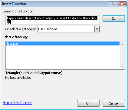
You can save yourself some keystrokes (and possible typing errors) by selecting your custom functions from the Insert Function dialog box. Your custom functions appear in the User Defined category:
An easier way to make your custom functions available at all times is to store them in a separate workbook and then save that workbook as an add-in. You can then make the add-in available whenever you run Excel. Here’s how to do this:
-
After you have created the functions you need, click File > Save As.
In Excel 2007, click the Microsoft Office Button, and click Save As
-
In the Save As dialog box, open the Save As Type drop-down list, and select Excel Add-In. Save the workbook under a recognizable name, such as MyFunctions, in the AddIns folder. The Save As dialog box will propose that folder, so all you need to do is accept the default location.
-
After you have saved the workbook, click File > Excel Options.
In Excel 2007, click the Microsoft Office Button, and click Excel Options.
-
In the Excel Options dialog box, click the Add-Ins category.
-
In the Manage drop-down list, select Excel Add-Ins. Then click the Go button.
-
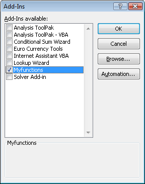
In the Add-Ins dialog box, select the check box beside the name you used to save your workbook, as shown below.

-
After you have created the functions you need, click File > Save As.
-
In the Save As dialog box, open the Save As Type drop-down list, and select Excel Add-In. Save the workbook under a recognizable name, such as MyFunctions.
-
After you have saved the workbook, click Tools > Excel Add-Ins.
-
In the Add-Ins dialog box, select the Browse button to find your add-in, click Open, then check the box beside your Add-In in the Add-Ins Available box.
After you follow these steps, your custom functions will be available each time you run Excel. If you want to add to your function library, return to the Visual Basic Editor. If you look in the Visual Basic Editor Project Explorer under a VBAProject heading, you will see a module named after your add-in file. Your add-in will have the extension .xlam.
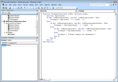
Double-clicking that module in the Project Explorer causes the Visual Basic Editor to display your function code. To add a new function, position your insertion point after the End Function statement that terminates the last function in the Code window, and begin typing. You can create as many functions as you need in this manner, and they will always be available in the User Defined category in the Insert Function dialog box.
This content was originally authored by Mark Dodge and Craig Stinson as part of their book Microsoft Office Excel 2007 Inside Out. It has since been updated to apply to newer versions of Excel as well.
Need more help?
You can always ask an expert in the Excel Tech Community or get support in the Answers community.
Need more help?
![]()
Download Article
![]()
Download Article
Microsoft Excel has many built-in functions, such as SUM, VLOOKUP, and LEFT. As you start using Excel for more complicated tasks, you may find that you need a function that doesn’t exist. That’s where custom functions come in! This wikiHow teaches you how to create your own functions in Microsoft Excel.
-
1
Open an Excel workbook. Double-click the workbook in which you want to use the custom-defined function to open it in Excel.
-
2
Press Alt+F11 (Windows) or Fn+⌥ Opt+F11 (Mac). This opens the Visual Basic Editor.
Advertisement
-
3
Click the Insert menu and select New Module. This opens a module window in the right panel of the editor.[1]
- You can create the user defined function in the worksheet itself without adding a new module, but that will make you unable to use the function in other worksheets of the same workbook.
-
4
Create your function’s header. The first line is where you will name the function and define our range.[2]
Replace «FunctionName» with the name you want to assign your custom function. The function can have as many parameters as you want, and their types can be any of Excel’s basic data or object types as Range:Function FunctionName (param1 As type1, param2 As type2 ) As return Type
- You may think of parameters as the «operands» your function will act upon. For example, when you use SIN(45) to calculate the Sine of 45 degree, 45 will be taken as a parameter. Then the code of your function will use that value to calculate something else and present the result.
-
5
Add the code of the function. Make sure you use the values provided by the parameters, assign the result to the name of the function, and close the function with «End Function.» Learning to program in VBA or in any other language can take some time and a detailed tutorial. However, functions usually have small code blocks and use very few features of the language. Some useful elements are:
- The If block, which allows you to execute a part of the code only if a condition is met. Notice the elements in an If code block: IF condition THEN code ELSE code END IF. The Else keyword along with the second part of the code are optional:
Function Course Result(grade As Integer) As String
  If grade >= 5 Then
    CourseResult = "Approved"
  Else
    CourseResult = "Rejected"
  End If
End Function
- The Do block, which executes a part of the code While or Until a condition is met. In the example code below, notice the elements DO code LOOP WHILE/UNTIL condition. Also notice the second line in which a variable is declared. You can add variables to your code so you can use them later. Variables act as temporary values inside the code. Finally, notice the declaration of the function as BOOLEAN, which is a datatype that allows only the TRUE and FALSE values. This method of determining if a number is prime is by far not the optimal, but I’ve left it that way to make the code easier to read.
Function IsPrime(value As Integer) As Boolean
  Dim i As Integer
  i = 2
  IsPrime = True
  Do
    If value / i = Int(value / i) Then
      IsPrime = False
    End If
    i = i + 1
  Loop While i < value And IsPrime = True
End Function
- The For block executes a part of the code a specified number of times. In this next example, you’ll see the elements FOR variable = lower limit TO upper limit code NEXT. You’ll also see the added ElseIf element in the If statement, which allows you to add more options to the code that is to be executed. Additionally, the declaration of the function and the variable result as Long. The Long datatype allows values much larger than Integer:
Public Function Factorial(value As Integer) As Long
  Dim result As Long
  Dim i As Integer
  If value = 0 Then
    result = 1
  ElseIf value = 1 Then
    result = 1
  Else
    result = 1
    For i = 1 To value
      result = result * i
    Next
  End If
  Factorial = result
End Function
- The If block, which allows you to execute a part of the code only if a condition is met. Notice the elements in an If code block: IF condition THEN code ELSE code END IF. The Else keyword along with the second part of the code are optional:
-
6
Close the Visual Basic Editor. Once you’ve created your function, close the window to return to your workbook. Now you can start using your user-defined function.
-
7
Enter your function. First, click the cell in which you want to enter the function. Then, click the function bar at the top of Excel (the one with the fx to its left) and type =FUNCTIONNAME(), replacing FUNCTIONNAME with the name you assigned your custom function.
- You can also find your user-defined formula in the «User Defined» category in the Insert Formula wizard—just click the fx to pull up the wizard.
-
8
Enter the parameters into the parentheses. For example, =NumberToLetters(A4). The parameters can be of three types:
- Constant values typed directly in the cell formula. Strings have to be quoted in this case.
- Cell references like B6 or range references like A1:C3. The parameter has to be of the Range datatype.
- Other functions nested inside your function. Your function can also be nested inside other functions. Example: =Factorial(MAX(D6:D8)).
-
9
Press ↵ Enter or ⏎ Return to run the function. The results will display in the selected cell.


Advertisement
Add New Question
-
Question
How can I use these functions in all Excel files?

Igal Livne
Community Answer
Save the workbook with the custom class as «Excel Add-In (*.xlam»),» by default Excel will take you to «Addins» folder. Go to Excel Options > Add-ins > Manage: «Excel Addins» — press «Go…» button. Browse for your newly create xlam file.
-
Question
How can I do well in exams?
Read the directions several times, leaving time for you to absorb between readings. Also practice writing VBA to do various things.
-
Question
How do I know what to write as the function code?
In order to create functions, you need a skill called «programming». Excel macros are written in a language called «Visual Basic for Applications», which you will need to learn to be able to write macros. It’s quite easy once you’ve got the hang of it though!
Ask a Question
200 characters left
Include your email address to get a message when this question is answered.
Submit
Advertisement
Video
-
Use a name that’s not already defined as a function name in Excel or you’ll end up being able to use only one of the functions.
-
Whenever you write a block of code inside a control structure like If, For, Do, etc. make sure you indent the block of code using a few blank spaces or the Tab key. That will make your code easier to understand and you’ll find a lot easier to spot errors and make improvements.
Show More Tips
Thanks for submitting a tip for review!
Advertisement
-
The functions used in this article are, by no means, the best way to solve the related problems. They were used here only to explain the usage of the control structures of the language.
-
VBA, as any other language, has several other control structures besides Do, If and For. Those have been explained here only to clarify what kind of things can be done inside the function source code. There are many online tutorials available where you can learn VBA.
-
Due to security measures, some people may disable macros. Make sure you let your colleagues know the book you’re sending them has macros and that they can trust they’re not going to damage their computers.
Advertisement
About This Article
Article SummaryX
1. Open Excel.
2. Press Alt + F11 to open the Visual Basic editor.
3. Create the function’s name and set the parameter types.
4. Use VB code to write your function.
5. Close the editor.
6. Run your function as you would other functions.
Did this summary help you?
Thanks to all authors for creating a page that has been read 640,306 times.
Is this article up to date?
Spreadsheets aren’t merely for arranging data into rows and columns. Most of the time, you use them for data analysis as well.
Microsoft Excel is one of the most widely used spreadsheet applications, especially in finance and accounting. This is partly because of its easy UI and unmatched depth of functions.
In this article, you will learn:
- What Excel formulas are
- How to write a formula in Excel
- What Excel functions are
- How to work with an Excel function
- Lastly, we’ll take a look at dynamic Excel functions.
What do I need to install on my computer to follow this article?
To follow along, you will need to have Microsoft Excel installed on your computer. We’ll use a Windows computer for this article.
How can I install Microsoft Excel on my computer?
Follow these steps to install Microsoft Excel on your Windows computer:
- Sign in to www.office.com if you’re not already signed in.
- Sign in with the account associated with your Microsoft 365 subscription. You can also try out Office for free as well.
- Once signed in, select “Install Office” from the Office home page. This will automatically download Microsoft Office onto your Windows computer.
- Run the installer to set up Microsoft Office and select «Close» once you’re done.
- Once done, select the “Start” button (located at the lower-left corner of your screen) and type “Microsoft Excel.”
- Click on Microsoft Excel to open it.
- Accept the license agreement, and let’s get started.
What are Excel Formulas?
An Excel formula is an expression that carries out an operation based on the value of a cell or range of cells. You can use an Excel formula to:
- Perform simple mathematical operations such as addition or subtraction.
- Perform a simple operation like joining categorical data.
It’s important to understand two things: Excel formulas always begin with the equals «=» sign and they can return an error if not properly executed.
What Operators Are Used in Excel Formulas?
There are four different types of operators in Excel—arithmetic, comparison, text concatenation, and reference. But for most formulas, you’ll typically use these three:
Arithmetic operators
|
+ |
Addition |
|
— |
Subtraction |
|
/ |
Division |
|
* |
Multiplication |
|
^ |
Exponentiation |
Comparison operators
|
= |
Equal to |
|
> |
Greater than |
|
< |
Less than |
|
>= |
Greater than or equal to |
|
<= |
Less than or equal to |
|
<> |
Not equal to |
Text concatenation
Here you have just the ampersand “&” sign for joining text.
How Can I Create an Excel Formula?
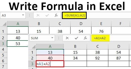
Let’s take a simple scenario using one of the arithmetic operators.
In math, to add up two numbers, let’s say 20 and 30, you will calculate this by writing: 20 + 30 =
And this will give you 50.
In Excel, here is how it goes:
- First, open a blank Excel worksheet.
- In cell A1, type 20.
- In cell A2, type 30.
- To add it up, type in = 20 + 30 in cell A3.

5. Then, press ENTER on your keyboard. Excel will instantly calculate this and return 50.

I mentioned earlier that every formula begins with the equal «=» sign. That’s what I meant. To write a formula, you type the equal to sign followed by the numeric values. This also applies to cases of subtraction, division, multiplication, and exponentiation.
Let’s take another simple scenario using one of the comparison operators. Assume we want to find out if 30 is greater than 40.
In Excel, here is how we would do it:
- Type in =30>40
- Press ENTER.

3. This will return a FALSE because 30 isn’t greater than 40. Excel uses TRUE and FALSE for logical statements, the same way we human says yes and no.

Lastly, let’s take another simple scenario using the text concatenation operator – the ampersand “&” sign. This works with your string data types and you use it to join text.
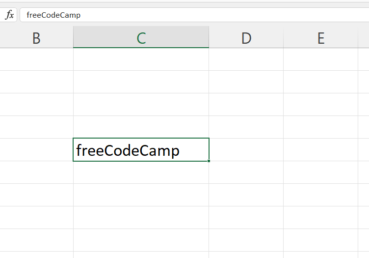
Assume we have «Welcome», «To», and «FreeCodeCamp» all in different cells—A1, A2, and A3—of your worksheet. We would type =A1&” “&A2&” “&A3 to join them.
The space in quotes “ “ represents that we want a space between our words.

Another tip: the formula bar shows the formula used to generate a value.
What Are Excel Functions?
Excel functions are predefined inbuilt formulas that perform mathematical, statistical, and logical calculations and operations using your values and arguments.
For Excel functions, you should know that:
- They’re formulas, so yeah, they start with the equal «=» sign as well.
- The order is very important.
There are over 500 functions available. You can find all available Excel functions on the Formulas tab on the Ribbon.

But why use a function when you can just write a formula?
Here are some benefits of Excel functions.
- To improve productivity and effectiveness.
- To simplify complex calculations.
- To automate your work.
- To quickly visualize data.
What Makes Up Excel Functions?
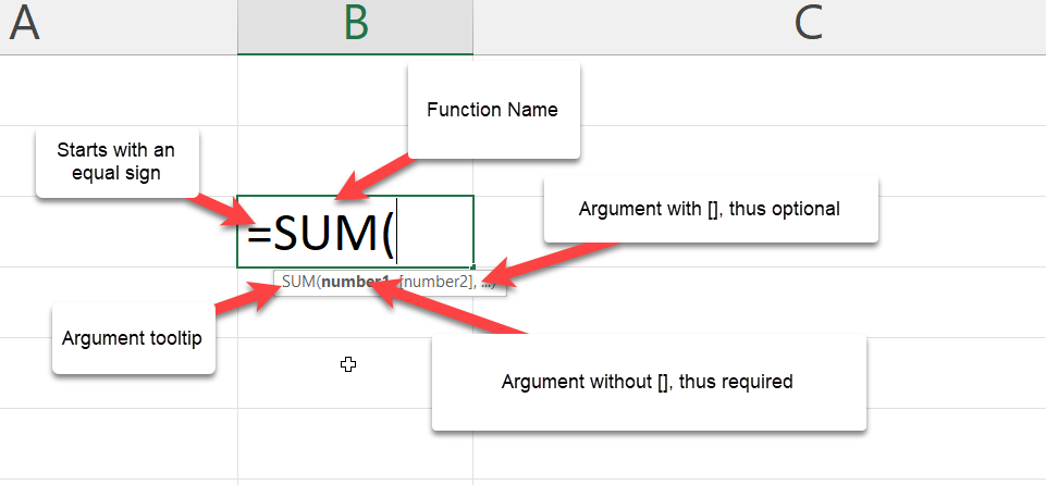
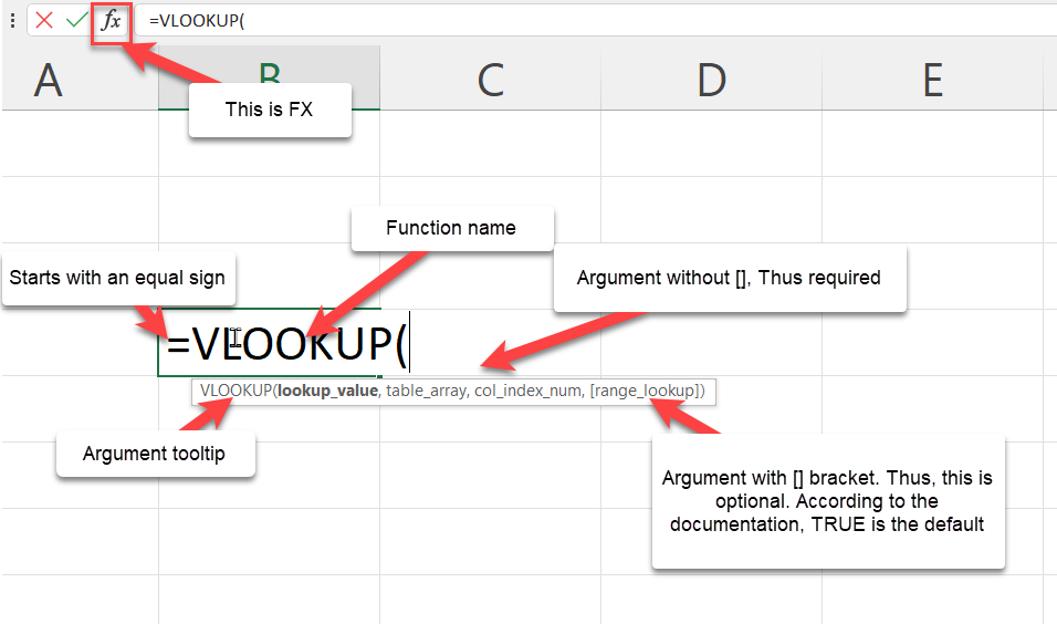
Unlike formulas, Excel functions are made up of a structure with arguments you need to pass.
Every function:
- Starts with the equals «=» sign
- Has a name. Some examples are VLOOKUP, SUM, UNIQUE, and XLOOKUP.
- Requires arguments which are separated by commas. You should know that semicolons are used as separators in countries like Spain, France, Italy, Netherlands, and Germany. You can, however, change this via the Excel setting.
- Argument with the square brackets [] are optional
- Has an opening and closing parenthesis.
- Has an argument tooltip which shows you what you should pass.
There are some exceptions. For example,
- The DATEDIF doesn’t show in Excel because it is not a standard function and gives incorrect results in a few circumstances. However, here is the syntax:
DATEDIF(birthdate, TODAY(), "y")
- Functions like PI(), RAND(), NOW(), TODAY() require no argument.
Let’s look at a few functions:
How to Use the SUM() Function in Excel
According to the documentation, the SUM function adds values. Here is the syntax:
Let’s assume that we have a line of numbers from 1 to 10 and we want to add it up. To achieve this, we will just type =SUM(A1:A10). The A1:A10 simply returns an array of number that are situated on cell A1 to A10 which are A1, A2, and A3 up through A10.

Since the second argument is optional, that means a sum(A10) will return a value. In our case, it will return just 10 since A10 has the value 10 in it. Give it a try.
If you were writing this using the addition operator, you would have written:
=1 + 2 + 3 + 4 + 5 + 6 + 7 + 8 + 9 + 10
or
=A1 + A2 + A3 + A4 + A5 + A6 + A7 + A8 + A9 + A10
This doesn’t look very productive or efficient.
How to Use the TODAY() Function in Excel
According to the documentation, the TODAY function displays the current date on your worksheet. It also requires no argument. Here is the syntax:

Excel displays the current date automatically according to your computer’s date and time setting. The same goes for the NOW() function, which displays the current date and time.
How to Use the CONCATENATE() Function in Excel
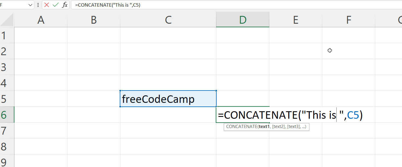
Let’s look at a text function. You use CONCATENATE to join two or more text strings into one string together.
Here is the syntax:

Let’s assume we want to join “This is” with “freeCodeCamp” – but in your cell, you have just «freeCodeCamp.»
If you’re going to write a string inside a formula, you must write it inside quotes like this “ “.
Why?
This way, Excel wouldnt think you’re trying to write another function.
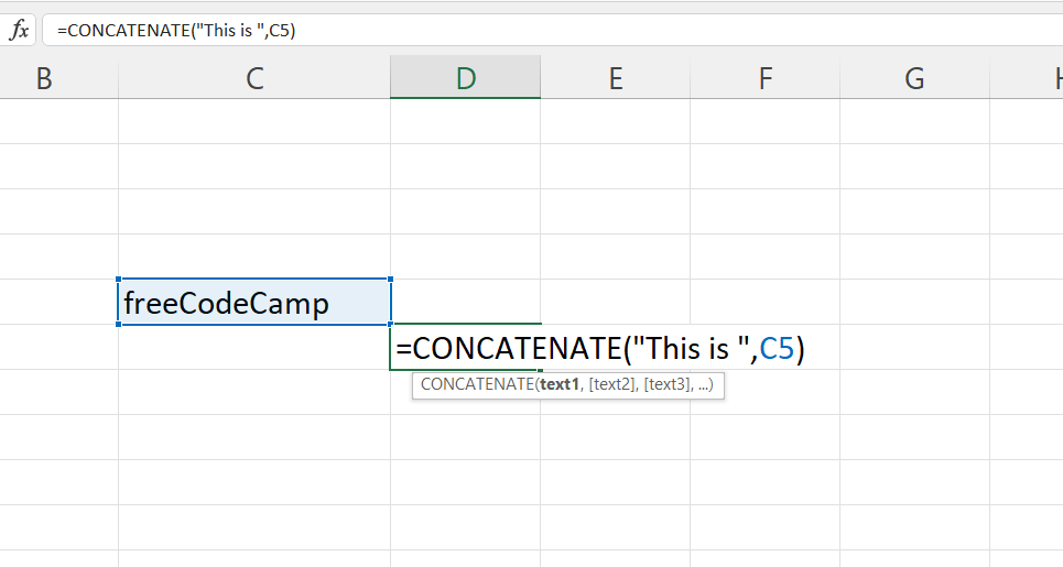
This will return the phrase “This is freeCodeCamp”
How to Use the VLOOKUP() Function in Excel
This is one of Excel’s most interesting and commonly used formulas or functions. You use it to find a value in a table or range by row.
Here is a scenario:
We have a simple table that shows various films along with their genre, lead studio, audience score %, profitability, rotten tomatoes %, worldwide gross and year. I would use just the first 10 rows of the sample data from this GitHub Gist.

I want that, whenever I type in a movie in the yellow cell, the year should get displayed in the green cell. Let’s use VLOOKUP to find it.
This is the VLOOKUP syntax:
Besides writing your formulas in the cell, you can also write them using the Excel Insert Function (fx) button, which is close to the formula bar.
Let’s try this.
- Write
=Vlookup(on the green cell. - Click on fx. A dialogue box will pop up showing all the arguments this formula needs.
- Input the value for each argument.
- Lookup_value (required argument): This is what you want to find. In our case, that is the movie “Youth in Revolt” which is in cell B1.
- Table_array (required argument): This is just asking you for the table that contains the data. You give it the entire table, which in our case is A4:H13
- Col_index_num (required argument): This is asking you for the column number of the table you gave. In our case, we want the year. This is in column 8.
- Range_lookup (optional argument): Lastly, we pick if we want an approximate match (TRUE) or an exact match (FALSE).
— TRUE means approximate match, so it returns the closest or an estimate.
— FALSE means exact match, so it returns an error if it’s not found.
8. We would go for the FALSE because we want the exact match.

9. Click on «OK.» Excel will return 2010.
However, you can write this in the cell by typing in =VLOOKUP(B1,A4:H13,8,FALSE) in your cell.

Tips and Rules When Writing Excel Functions
When writing our function, Excel provides some formula tips.
- The Argument tooltip doesn’t leave until you close the last parenthesis.
- The formula bar shows your formula.
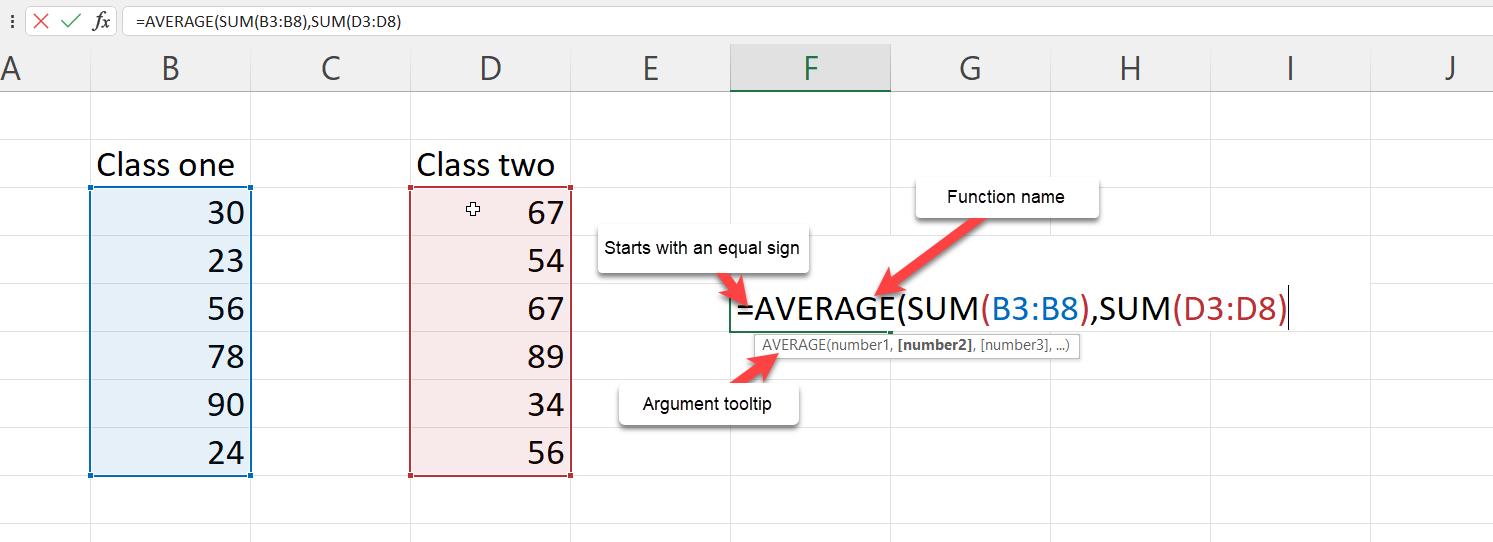
- The argument you are currently writing is always dark. Take a look at the lookup_value in the image below.
- The square brackets [] tell you it is optional.
- Lastly, the colour code – our B1 is in blue, and cell B1 is in blue to guide us on what cell or table was picked. The same thing will happen to A4:H13 when we pick it as our table_array argument.

How to Work with Nested Functions in Excel
A nested function is when you write a function within another function. For example, finding the average of the sum of values.
The first tip when writing a nested function will be to treat every function individually. So address the first function before addressing the second. A pro tip would be to look at the argument tooltip when writing it.
Let’s take a simple scenario.
We have two arrays of numbers. Each has the scores of students in the class. I want to add the two arrays before I get the average.
Let’s get started.
- Type in your = followed by the average.
- The number one will be the sum of the scores from class one.
- The number two will be the sum of the scores from class two.

Finally, don’t forget the closing parenthesis.
Thus, the formula will be =AVERAGE(SUM(B3:B8),SUM(D3:D8)).
How to Work with Dynamic Array Functions in Excel
Dynamic array functions are formulas associated with spill array behaviour.
Before now, you wrote a function and it returned just a single input. We call these kinds of functions legacy array formulas.
Dynamic array functions, on the other hand, will return values that will enter the neighbouring cells. A few examples of dynamic array functions are:
- UNIQUE
- TEXTSPLIT
- FILTER
- SEQUENCE
- SORT
- SORTBY
- RANDARRAY
Let’s look at the UNIQUE formula.
How to Use the UNIQUE() Formula in Excel
The unique formula works by returning the unique value from an array or list. Let’s use the movie sample data from this GitHub Gist. This table contains 77 rows of film excluding the heading.

Let’s try to get the unique years from our dataset – that is, years without duplicates.
To do this:
- Type
=UNIQUE( - Select the entire array of values from the year column: =UNIQUE(H2:H78)

3. Close the parenthesis and press Enter.
Though the formula was written in a single cell, the returned value got spilled into the cells below it. That’s the spilled array behaviour.

How to Create Your Own Functions in Excel
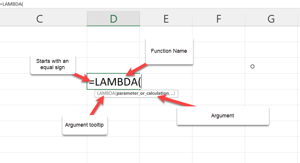
Microsoft Excel released a bunch of new functions to make user more productive. One of these function was the LAMBDA function.
The LAMBDA function lets you create custom functions without macros, VBA or JavaScript, and reuse them throughout a workbook.
The best part? you can name it.
How to Use the LAMBDA() Function in Excel
This LAMBDA function will increase productivity by eliminating the need to copy and paste this formula, which can be error-prone.
Here is the LAMBDA syntax:
Lets start with a simple use case using the movie sample data from this GitHub Gist.
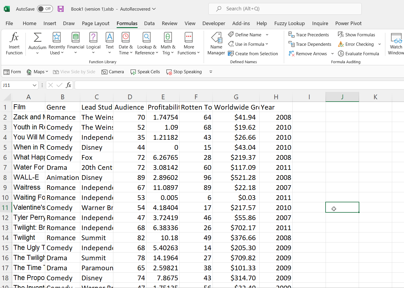
We had a column called «Worldwide Gross», lets try to find the Naira value.
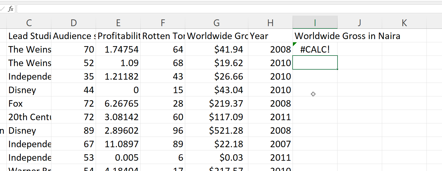
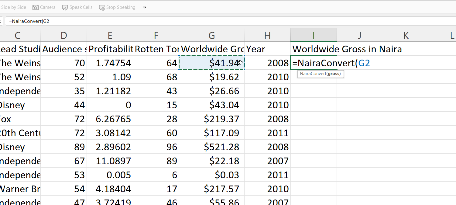
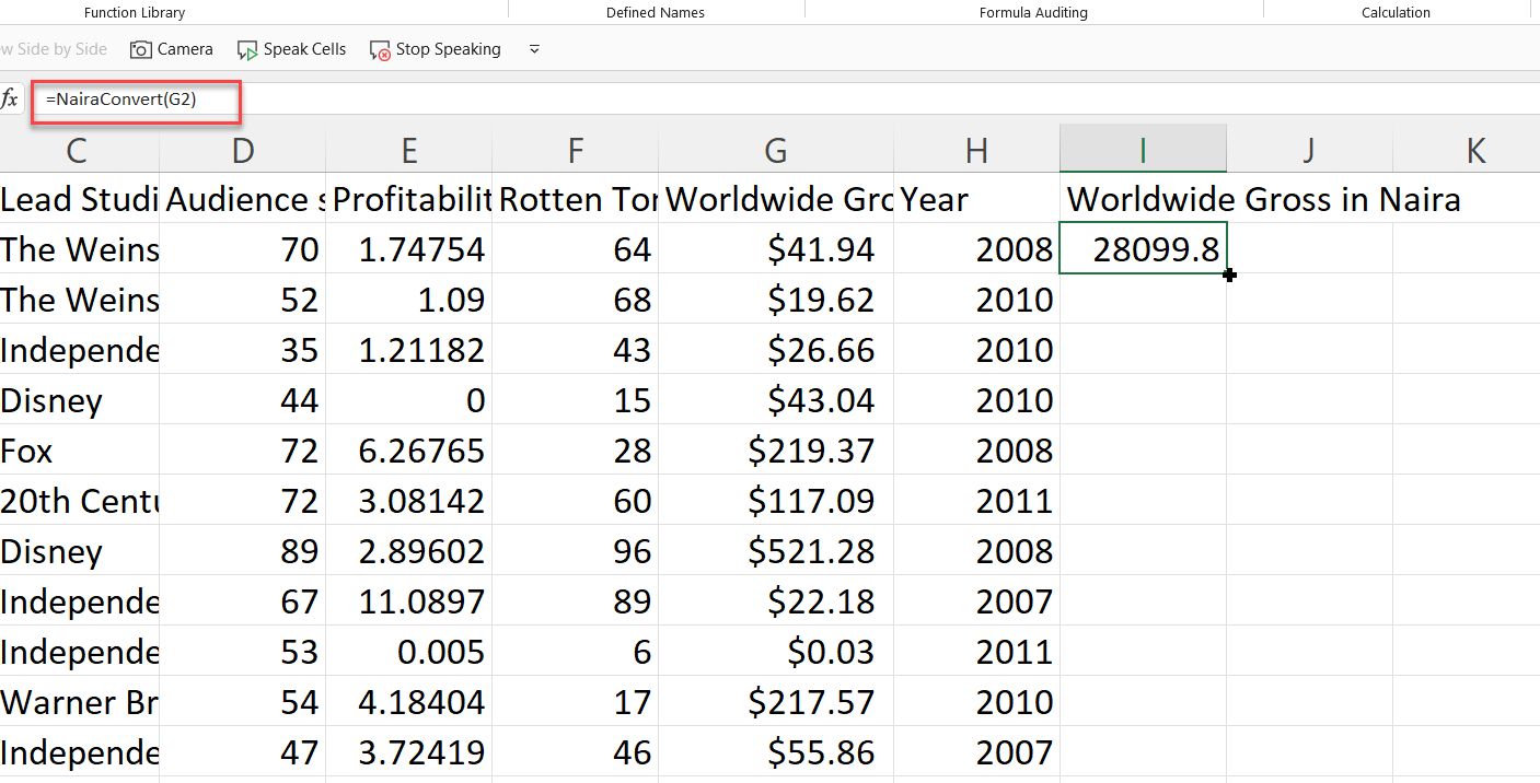
- Create a new column and call it «Worldwide Gross in Naira».
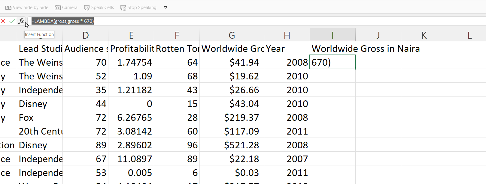
- Right below our column name, Cell I2, type
=lAMBDA( - LAMBDA requires a parameter and/or a calculation.
The parameter means the value you want to pass, in our use case we want to change the gross value. Lets call it gross.
The calculation means the formula or function you want to execute. For us, that will be to multiply it with te exchange rate. At the moment, that’s 670. so lets write gross * 670.
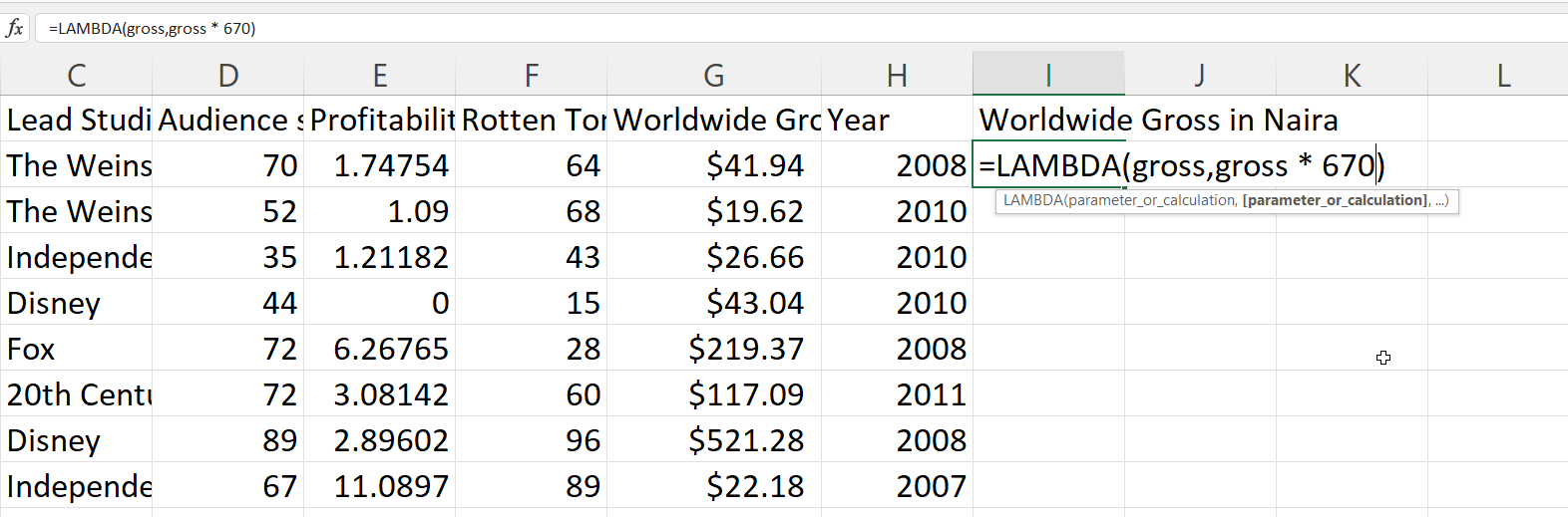
4. Press Enter. This will return an error because, gross doesnt exist and you need to let excel know of these names.
5. To make use of the newly created function, you need to copy the syntax written.
6. Go to the formula ribbon and open the name manager.
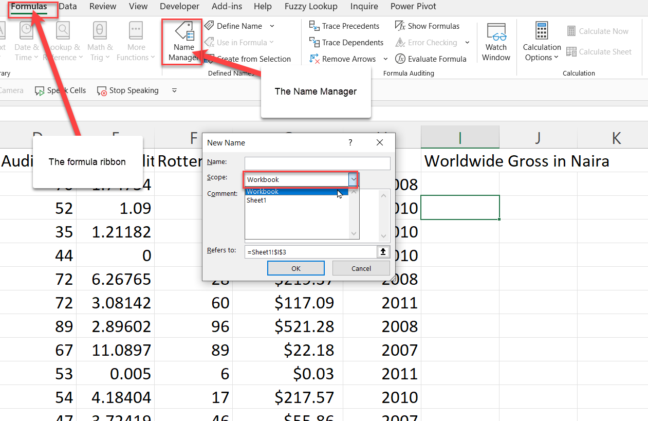
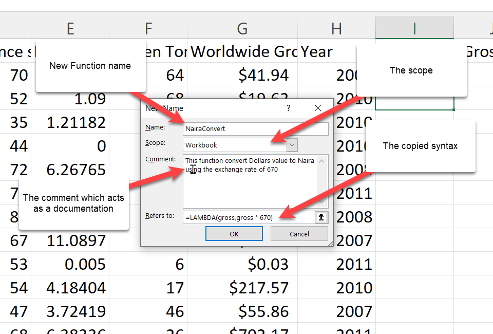
7. Define the name manger parameters:
- The name is simply what you want to call this function. I am going with NairaConvert.
- The scope should be workbook because you want to use this function in the workbook.
- The comments explains what your function does. It is acts as a documentation.
- In the refer to, you should paste the copied function syntax.
8. Press Ok.
9. To use this new function, you call it with the name you defined it as—NairaConvert—and give it the gross which is our worldwise gross on G2.
10. Close the parenthesis and press Ok
Where Can I Learn More about Excel?
There are a ton of resources for learning Microsoft Excel nowadays. So many that it is hard to figure out which ones are up-to-date and helpful.
The best thing you can do is find a helpful tutorial and follow it to completion, instead of attempting to take several at once. I would advise you to start with freeCodeCamp’s Microsoft Excel Tutorial for Beginners — Full Course, which is available on YouTube.
You should also join communities like the Microsoft Excel and Data Analysis Learning Community. However, if you’re looking for a compilation of resources, check out freeCodeCamp’s publication Excel tags.
If you enjoyed reading this article and/or have any questions and want to connect, you can find me on LinkedIn or Twitter.
Learn to code for free. freeCodeCamp’s open source curriculum has helped more than 40,000 people get jobs as developers. Get started
In this tutorial we will learn about Excel VBA function
1) What is Visual Basic in Excel?
2) How to use VBA in Excel?
3) How to create User defined function?
4) How to write Macro?
How to write VBA code
Excel provides the user with a large collection of ready-made functions, more than enough to satisfy the average user. Many more can be added by installing the various add-ins that are available. Most calculations can be achieved with what is provided, but it isn’t long before you find yourself wishing that there was a function that did a particular job, and you can’t find anything suitable in the list. You need a UDF. A UDF (User Defined Function) is simply a function that you create yourself with VBA. UDFs are often called «Custom Functions». A UDF can remain in a code module attached to a workbook, in which case it will always be available when that workbook is open. Alternatively you can create your own add-in containing one or more functions that you can install into Excel just like a commercial add-in. UDFs can be accessed by code modules too. Often UDFs are created by developers to work solely within the code of a VBA procedure and the user is never aware of their existence. Like any function, the UDF can be as simple or as complex as you want. Let’s start with an easy one…
A Function to Calculate the Area of a Rectangle
Yes, I know you could do this in your head! The concept is very simple so you can concentrate on the technique. Suppose you need a function to calculate the area of a rectangle. You look through Excel’s collection of functions, but there isn’t one suitable. This is the calculation to be done:
AREA = LENGTH x WIDTH
Open a new workbook and then open the Visual Basic Editor (Tools > Macro > Visual Basic Editor or ALT+F11).
You will need a module in which to write your function so choose Insert > Module. Into the empty module type: Function Area and press ENTER.The Visual Basic Editor completes the line for you and adds an End Function line as if you were creating a subroutine.So far it looks like this…
Function Area()

End Function
Place your cursor between the brackets after «Area». If you ever wondered what the brackets are for, you are about to find out! We are going to specify the «arguments» that our function will take (an argument is a piece of information needed to do the calculation). Type Length as double, Width as double and click in the empty line underneath. Note that as you type, a scroll box pops-up listing all the things appropriate to what you are typing.

This feature is called Auto List Members. If it doesn’t appear either it is switched off (turn it on at Tools > Options > Editor) or you might have made a typing error earlier. It is a very useful check on your syntax. Find the item you need and double-click it to insert it into your code. You can ignore it and just type if you want. Your code now looks like this…
Function Area(Length As Double, Width As Double)

End Function
Declaring the data type of the arguments is not obligatory but makes sense. You could have typed Length, Width and left it as that, but warning Excel what data type to expect helps your code run more quickly and picks up errors in input. The double data type refers to number (which can be very large) and allows fractions. Now for the calculation itself. In the empty line first press the TAB key to indent your code (making it easier to read) and type Area = Length * Width. Here’s the completed code…
Function Area(Length As Double, Width As Double)
    Area = Length * Width
End Function
You will notice another of the Visual Basic Editor’s help features pop up as you were typing, Auto Quick Info…

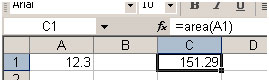
It isn’t relevant here. Its purpose is to help you write functions in VBA, by telling you what arguments are required. You can test your function right away. Switch to the Excel window and enter figures for Length and Width in separate cells. In a third cell enter your function as if it were one of the built-in ones. In this example cell A1 contains the length (17) and cell B1 the width (6.5). In C1 I typed =area(A1,B1) and the new function calculated the area (110.5)…

Sometimes, a function’s arguments can be optional. In this example we could make the Width argument optional. Supposing the rectangle happens to be a square with Length and Width equal. To save the user having to enter two arguments we could let them enter just the Length and have the function use that value twice (i.e. multiply Length x Length). So the function knows when it can do this we must include an IF Statement to help it decide. Change the code so that it looks like this…
Function Area(Length As Double, Optional Width As Variant)
    If IsMissing(Width) Then
        Area = Length * Length
    Else
        Area = Length * Width
    End If
End Function
Note that the data type for Width has been changed to Variant to allow for null values. The function now allows the user to enter just one argument e.g. =area(A1).The IF Statement in the function checks to see if the Width argument has been supplied and calculates accordingly…
A Function to Calculate Fuel Consumption
I like to keep a check on my car’s fuel consumption so when I buy fuel I make a note of the mileage and how much fuel it takes to fill the tank. Here in the UK fuel is sold in litres. The car’s milometer (OK, so it’s an odometer) records distance in miles. And because I’m too old and stupid to change, I only understand MPG (miles per gallon). Now if you think that’s all a bit sad, how about this. When I get home I open up Excel and enter the data into a worksheet that calculates the MPG for me and charts the car’s performance. The calculation is the number of miles the car has travelled since the last fill-up divided by the number of gallons of fuel used…
MPG = (MILES THIS FILL — MILES LAST FILL) / GALLONS OF FUEL
but because the fuel comes in litres and there are 4.546 litres in a gallon..
MPG = (MILES THIS FILL — MILES LAST FILL) / LITRES OF FUEL x 4.546
Here’s how I wrote the function…
Function MPG(StartMiles As Integer, FinishMiles As Integer, Litres As Single)
    MPG = (FinishMiles - StartMiles) / Litres * 4.546
End Function
and here’s how it looks on the worksheet…

Not all functions perform mathematical calculations. Here’s one that provides information…
A Function That Gives the Name of the Day
I am often asked if there is a date function that gives the day of the week as text (e.g. Monday). The answer is no*, but it’s quite easy to create one. (*Addendum: Did I say no? Check the note below to see the function I forgot!). Excel has the WEEKDAY function, which returns the day of the week as a number from 1 to 7. You get to choose which day is 1 if you don’t like the default (Sunday). In the example below the function returns «5» which I happen to know means «Thursday».

But I don’t want to see a number, I want to see «Thursday». I could modify the calculation by adding a VLOOKUP function that referred to a table somewhere containing a list of numbers and a corresponding list of day names. Or I could have the whole thing self-contained with multiple nested IF statements. Too complicated! The answer is a custom function…
Function DayName(InputDate As Date)
    Dim DayNumber As Integer
    DayNumber = Weekday(InputDate, vbSunday)
    Select Case DayNumber
        Case 1
            DayName = "Sunday"
        Case 2
            DayName = "Monday"
        Case 3
            DayName = "Tuesday"
        Case 4
            DayName = "Wednesday"
        Case 5
            DayName = "Thursday"
        Case 6
            DayName = "Friday"
        Case 7
            DayName = "Saturday"
    End Select
End Function
I’ve called my function «DayName» and it takes a single argument, which I call «InputDate» which (of course) has to be a date. Here’s how it works…
- The first line of the function declares a variable that I have called «DayNumber» which will be an Integer (i.e. a whole number).
- The next line of the function assigns a value to that variable using Excel’s WEEKDAY function. The value will be a number between 1 and 7. Although the default is 1=Sunday, I’ve included it anyway for clarity.
- Finally a Case Statement examines the value of the variable and returns the appropriate piece of text.
Here’s how it looks on the worksheet…

Accessing Your Custom Functions
If a workbook has a VBA code module attached to it that contains custom functions, those functions can be easily addressed within the same workbook as demonstrated in the examples above. You use the function name as if it were one of Excel’s built-in functions.
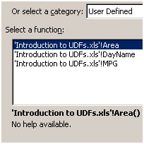
You can also find the functions listed in the Function Wizard (sometimes called the Paste Function tool). Use the wizard to insert a function in the normal way (Insert > Function).
Scroll down the list of function categories to find User Defined and select it to see a list of available UDFs…


You can see that the user defined functions lack any description other than the unhelpful «No help available» message, but you can add a short description…
Make sure you are in the workbook that contains the functions. Go to Tools > Macro > Macros. You won’t see your functions listed here but Excel knows about them! In the Macro Name box at the top of the dialog, type the name of the function, then click the dialog’s Options button. If the button is greyed out either you’ve spelled the function name wrong, or you are in the wrong workbook, or it doesn’t exist! This opens another dialog into which you can enter a short description of the function. Click OK to save the description and (here’s the confusing bit) click Cancel to close the Macro dialog box. Remember to Save the workbook containing the function. Next time you go to the Function Wizard your UDF will have a description…

Like macros, user defined functions can be used in any other workbook as long as the workbook containing them is open. However it is not good practice to do this. Entering the function in a different workbook is not simple. You have to add its host workbook’s name to the function name. This isn’t difficult if you rely on the Function Wizard, but clumsy to write out manually. The Function Wizard shows the full names of any UDFs in other workbooks…
If you open the workbook in which you used the function at a time when the workbook containing the function is closed, you will see an error message in the cell in which you used the function. Excel has forgotten about it! Open the function’s host workbook, recalculate, and all is fine again. Fortunately there is a better way.
If you want to write User Defined Functions for use in more than one workbook the best method is to create an Excel Add-In. Find out how to do this in the tutorial Build an Excel Add-In.
Addendum
I really ought to know better! Never, ever, say never! Having told you that there isn’t a function that provides the day’s name, I have now remembered the one that can. Look at this example…
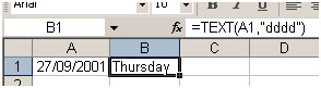
The TEXT function returns the value of a cell as text in a specific number format. So in the example I could have chosen =TEXT(A1,»ddd») to return «Thu», =TEXT(A1,»mmmm») to return «September» etc. The Excel’s help has some more examples of ways to use this function.
If you liked our blogs, share it with your friends on Facebook. And also you can follow us on Twitter and Facebook.
We would love to hear from you, do let us know how we can improve, complement or innovate our work and make it better for you. Write us at info@exceltip.com
Microsoft Excel’s table structure is a great way to keep organized. But the program is much more than just a series of rows and columns into which you can enter data.
Excel really becomes powerful once you start using functions, which are mathematical formulas that help you quickly and easily make calculations that would be difficult to do by hand.
Functions can do many things to speed up your calculations. For example, you could use functions to take the sum of a row or column of data; find the average of a series of numbers; output the current date; find the number of orders placed by a particular customer within a given period of time; look up the e-mail address of a customer based on his or her name; and much more. It’s all automatic — no manual entry required.
Let’s take a closer look at functions to see how they work.
The structure of a function
Think of a function like a recipe: you put together a series of ingredients, and the recipe spits out something totally new and different (and, in most cases, more useful, or delicious, than the thing that you put in). Like recipes, functions have three key pieces that you should keep track of:
- First, there’s the function name. This is just like the recipe name that you would see at the top of one of the pages of your cookbook. It is a unique identifier that tells Excel what we are trying to cook up.
- Next, there are arguments. Arguments are just like the ingredients of a recipe. They’re pieces that you put in that will eventually combine to make something bigger.
- Finally, there’s the output. The output of a function is just like the output of a recipe — it’s the final product that is ready to be presented to the user (or, in the case of a recipe, eaten).
Writing a function in Excel
When we enter functions into Excel, we use a special character to tell the program that what we are entering is a function and not a normal block of text: the equals sign (=). Whenever Excel sees the = sign at the beginning of the input to a cell, it recognizes that we are about to feed it a function.
The basic structure of a function is as follows:
=FUNCTION_NAME(argument_1, argument_2, argument_3...)
Output: Output
After the = sign, we write the name of the function to tell Excel which recipe we want to use. Then, we use the open parentheses sign (() to tell the program that we’re about to give it a list of arguments.
We then list the arguments to the function, one by one, separated by commas, to tell Excel what ingredients we are using. Note that just like recipes, each function has its own specific number of arguments that it needs to receive. Some just take one argument; others take two or even more.
To finish writing a function, wrap up the list of arguments with the close parentheses sign ()) to tell Excel that you’re done writing the list of ingredients. Then press the Enter key to complete your entry. You’ll see that rather than displaying the text that you entered, Excel shows the output of your completed function.
A practical example
Let’s look at a practical example using the SUM function. This is one of Excel’s most-used recipes — it takes any number of arguments (all of which should be numerical), and spits out the sum of those arguments. The formula for SUM is as follows:
=SUM(number_1, number_2...)
To recap: the name of the function is SUM. The arguments are number_1, number_2, and as many additional numbers as you want to put in (this particular function takes an unlimited number of arguments, just like a recipe that gets better and better as you throw in more ingredients). When you’re done writing the function and press Enter, Excel will show you the output.
Try entering the following into a cell on a blank spreadsheet:
=SUM(3, 7)
Output: 10
Excel outputs 10, because the SUM of 3 and 7 is 10.
Here’s another example with even more arguments:
=SUM(1, 2, 3, 4, 5)
Output: 15
Here, Excel outputs 15, the SUM of 1, 2, 3, 4, and 5.
Infinite arguments and optional arguments
Throughout these pages, we’ll use a couple different types of notation to denote special cases within functions:
First, some functions, like SUM above, have a theoretically infinite number of arguments. For example, you can take the SUM of an infinite number of numerals. In cases like this, we use three dots (…) to denote an infinite number of additional arguments, like so:
=FUNCTION_NAME(argument_1, argument_2, argument_3...)
If a function has a finite number of arguments, you won’t see that … at the end, like this:
=FUNCTION_NAME(argument_1, argument_2)
Finally, some arguments to functions are optional, just like some ingredients of a recipe might be optional. If one or more arguments of a function are optional, we’ll follow them up with an (optional) designator like so:
=FUNCTION_NAME(argument_1, argument_2 (optional))
In most of our function tutorials, we’ll explain why something is optional and how you can use it.
That’s it! Now that you know what a function is, check out our tutorials on some of Excel’s logical functions to get rolling with Excel’s most powerful tool.
Explore the 5 must-learn ‘fundamentals’ of Excel
Getting started with Excel is easy. Sign up for our 5-day mini-course to receive easy-to-follow lessons on using basic spreadsheets.
- The basics of rows, columns, and cells…
- How to sort and filter data like a pro…
- Plus, we’ll reveal why formulas and cell references are so important and how to use them…
Comments
Excel Write Formula (Table of Contents)
- Writing Formula in Excel
- How to Write Formula in Excel?
Writing Formula in Excel
What would be your answer when I ask you, “What is Excel?” A tool that helps to store, slicing and dicing the data plus a tool that can help us calculate sums, percentages, interest rates, etc., right? The most essential as well as an important part of Excel is a formula. The formula is nothing but an equation that allows you to perform various calculations under Microsoft Excel. These formulae are the easiest way of calculation based on the given data. However, being new to Excel, you might not always be able to handle the Excel formulae. It is very easy and simple, though, to add formulae under Excel. This article will try to make you literate about how to write different formulae under Excel, and you will be master in applying the same after going through this article.
Let’s see how we can create/write a formula under Excel.
The first thing we should know is, every Excel formula starts with the equals to sign (‘=’) inside an Excel cell. After this sign, you can write the equation in which you want Excel to perform calculations or any inbuilt function name (Ex. SUM), which performs a calculation and returns the output in a given cell.
How to Write Formula in Excel?
Let’s understand How to Write the formula in excel with a few examples.
You can download this Write Formula Excel Template here – Write Formula Excel Template
Example #1
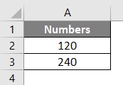
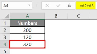
Step 1: Suppose we have two numbers, 120 and 240, in cell A1 and A2, respectively, in the Excel sheet. See the screenshot below:
Now, I want to add these two numbers; We’ll see how this can be achieved.
Step 2: In cell A4, start typing the equation by simply using equals to sign and then use 120 + 240 to add these two values up. See the screenshot below for a better understanding.
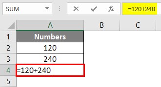
Step 3: Press Enter Key to see the result. You can see 360 as a result of cell A4, as shown below.
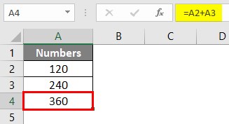
This is how a basic formula can be entered under Microsoft Excel. Now, what if we change the numbers in cell A1 and A2 to some different values? Will the formula under cell A3 change values? Well, let’s see by doing so.
Step 4: Change the numbers in cell A1 and A2 to 120 and 240, respectively.
If you will check cell A3, it is still showing the result for old values (i.e. 120 + 140 = 360). Because in cell A3, we have used the equation as 120 + 140. These are values that are fixed and not dynamic ones. Therefore, in order to get rid of such a situation, Excel also provides an option to be able to use dynamic ranges under an equation/formula for that sake.
Step 5: In cell A3, tweak the formula to =A2+ A3. What we tried doing here is, instead of giving a number as an argument, we have supplied the cells which contain a number as an argument. This will be beneficial when you change the numbers in cells A2, A3; values in cell A4 will automatically change after performing the operations. This is how making you formula dynamic using a range of cells work.
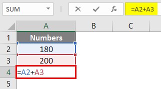
After using the above formula, the output is shown below:
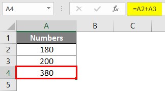
Now, if I change the values under cell A1 and A2, the results in cell A3 will automatically change. See the screenshot below.
Example #2
Excel has a more user-friendly approach when it comes to applying the formula. You just can simply copy-paste the formula from one cell to another by dragging it through. Let’s see how to do it.
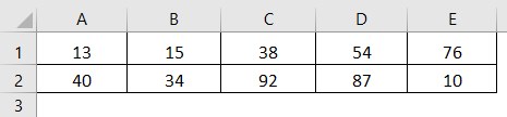
Suppose we have data as shown below across the first and second row of different columns (A to E), and we wanted to get a sum for each column in their third row, respectively. We’ll see how excel works in this situation.
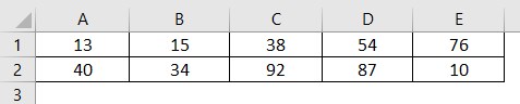
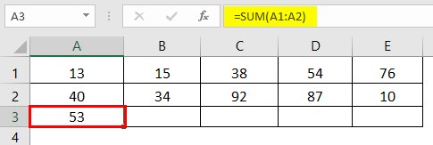
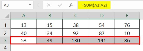
Step 1: In cell A3, create an equation using a dynamic range of cells that sums the values under A1 and A2. You can use =A1+A2 as a formula under cell A3 to get the sum of the numbers within those cells.
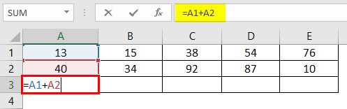
Also, Press Enter key to see the output in cell A3.
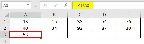
Step 2: Now, select the cell A3 and then drag the formula across A3 to E3 to apply the same formula that sums up the first and second row for each column. You should get the output as shown in the screenshot below:
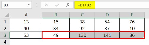
Well, you have multiple ways to achieve this result. You can select the entire third row across column A to E and just press Ctrl + R to copy and paste the formula under cell A3 to other columns. Or else, you can copy the formula under cell A3 by Ctrl + C and paste it one by one in each of B3, C3, D3, E3 to achieve the same result.
Example #3
In this example, we will work on using the built-in Excel functions. How to use the built-in Excel function to perform a task (ex. Summing number across the rows).
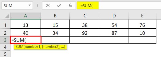
Consider the same data as shown in example 2, and we wanted to have sum of the first two rows of each column within the third row. However, this time we will use a built-in Excel function named SUM to achieve this result.
Step 1: In cell A3, start typing =SUM; it will pop up a list of all functions that contain SUM as a keyword. Select the SUM function through that list by double-clicking on it.
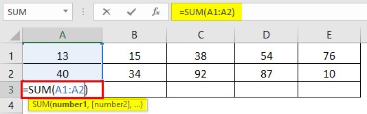
Step 2: Select the range of cells A1 to A2 with the use of your computer mouse or laptop touchpad as an argument to the SUM function. Because these are the cells that we wanted to sum up.
Well, you also can use the comma to separate the values instead of these ranges.
Step 3: Complete this formula by adding closing parentheses at the end of this function and press the Enter key to get the sum of cell A1 and A2 under cell A3.
This function precedes the equation we use in Example 2 by a huge margin when we have tons of data. Ex. Consider you have 5 Lacs Excel Rows, and you wanted to sum those up. You surely would not like to input each cell reference for 5 Lacs of time, would you?
Step 4: You can drag this formula across the different columns for the same row or user Ctrl + R to populate it across all the rows or copy and paste one by one to each column. The choice is all yours. You’ll get the final output as shown below:
This is it from this article. Let’s wrap the things up with some points to be remembered:
Things to Remember About Write Formula in Excel
- In order to be able to use a formula in Excel, you need to start it with equals to sign. You also can start a formula with a Plus or minus sign.
- You can have different operational formulae of your own for subtraction, multiplication, division, squaring a number, etc. However, all these operations are better to do with built-in Excel functions because these functions precede over operational formulae.
Recommended Articles
This is a guide to Write Formula in Excel. Here we discuss How to use Write Formula in Excel along with practical examples and a downloadable excel template. You can also go through our other suggested articles –
- Excel DEGREES Function
- Compare Two Lists in Excel
- Excel Text with Formula
- TIME in Excel
Write Basic Formulas in Excel
Formulas are an integral part of Excel. As a new learner of Excel, one does not understand the importance of formulas in Excel. However, all the new learners know plenty of built-in formulas but do not know how to apply them.
In this article, we will show you how to write formulas in Excel and dynamically change them when the referenced cell values are changed automatically.
Table of contents
- Write Basic Formulas in Excel
- How to Write/Insert Formulas in Excel?
- Example #1
- Example #2
- How to use Built-in Excel Functions?
- Example #1 – SUM Function
- Example #2 – AVERAGE Function
- Things to Remember about Inserting Formula in Excel
- Recommended Articles
- How to Write/Insert Formulas in Excel?

How to Write/Insert Formulas in Excel?
You can download this Write Formula Excel Template here – Write Formula Excel Template
To write a formula in Excel, you first need to enter the equal sign in the cell where we need to enter the formula. So, the formula always starts with an equal (=) sign.
Example #1
Look at the below data in the Excel worksheet.

We have two numbers in A1 and A2 cells, respectively. So, if we want to add these two numbers in cell A3, we must first open the equal sign in the A3 cell.

Enter the numbers as 525 + 800.

Press the “Enter” key to get the formula equation’s result.

The formula bar shows the formula, not the result of the formula.
As you can see above, we have got the result as 1325 as the summation of the numbers 525 and 800. In the formula bar, we can see how the formula has been applied = 525+800.
Now, we will change the A1 and A2 numbers to 50 and 80, respectively.

Result cell A3 shows the old formula result only. It is where we need to make dynamic cell referenceCell reference in excel is referring the other cells to a cell to use its values or properties. For instance, if we have data in cell A2 and want to use that in cell A1, use =A2 in cell A1, and this will copy the A2 value in A1.read more formulas.
Instead of entering the two cell numbers, give a cell reference only to the formula.

Press the “Enter” key to get the result of this formula.

In the formula bar, we can see the formula as A1 + A2, not the numbers of the A1 and A2 cells. Now, change the numbers of any of the cells. For example, in the A3 cell, it will automatically impact the result.

We have changed the A1 cell number from 50 to 100, and because the A3 cell has the reference of the cells A1 and A2, the A3 cell automatically changed.
Example #2
Now, we have other numbers for the adjacent columns.

We have numbers in four more columns. We need to get the total of these numbers as we did for A1 and A3 cells.

It is where the real power of cell-references formulas is crucial in making the formula dynamic. For example, copy cell A3, which has already applied the formula A1 + A2, and paste it to the next cell, B3.

Look at the result in cell B3. The formula bar says the formula as B1 + B2 instead of A1 + A2.
When we copied and pasted the A3 cell, the formula cell, we moved one column to the right. But in the same row, we have passed the formula. Because we moved one column to the right in the same row-column reference or header value, “A” has been changed to “B,” but row numbers 1 and 2 remain the same.
Copy and paste the formula to other cells to get the total in all the cells.

How to use Built-in Excel Functions?
Example #1 – SUM Function
We have plenty of built-in functions in Excel according to the requirements and situations we can use. For example, look at the below data in Excel.

We have numbers from the A1 to E5 range of cells. In the B7 cell, we need the total sum of these numbers. Adding individual cell references and entering each cell reference one by one consumes a lot of time, so putting an equal sign open SUM function in excelThe SUM function in excel adds the numerical values in a range of cells. Being categorized under the Math and Trigonometry function, it is entered by typing “=SUM” followed by the values to be summed. The values supplied to the function can be numbers, cell references or ranges.read more.

Select the range of cells from A1 to E5 and close the bracket.

Press the “Enter” key to get the total numbers from A1 to E5.

In just a fraction of seconds, we got the total numbers. In the formula bar, we can see the formula as =SUM(A1: E5).
Example #2 – AVERAGE Function
Assume you have students” every subject score, and you need to find the student’s average score. It is possible to find an average score in a fraction of seconds. For example, look at the below data.

Open AVERAGE function in the H2 cell first.

Select the range of cells reference as B2 to G2 because for the student “Amit,” all the subject scores are in this range only.

Press the “Enter” key to get the average student “Amit.”

So, the student “Amit” average score is 79.
Now, drag formula cell H2 to the below cells to get the average of other students.

Things to Remember about Inserting Formula in Excel
- The formula should always start with an equal sign. We can also start with a PLUS or MINUS sign but not recommended.
- While doing calculations, we need to remember BODMAS’s basic Maths rules.
- We must always use built-in functions in Excel.
Recommended Articles
This article is a guide to Write Formula in Excel. Here, we discuss how to insert formulas and built-in functions in Excel with examples and a downloadable Excel template. You may learn more about Excel from the following articles: –
- Evaluate Formula in ExcelThe Evaluate formula in Excel is used to analyze and understand any fundamental Excel formula such as SUM, COUNT, COUNTA, and AVERAGE. For this, you may use the F9 key to break down the formula and evaluate it step by step, or you may use the “Evaluate” tool.read more
- Marksheet in ExcelMarksheets in Excel help keep records, entries, and tracking the performance of students, candidates, and even employees and workers, thereby, reducing the task of regularizing hundreds of people to a more simple and easy way within the desired format.read more
- Excel Infographics
- Excel Hacks
Excel allows you to create custom functions using VBA, called «User Defined Functions» (UDFs) that can be used the same way you would use SUM() or other built-in Excel functions. They can be especially useful for advanced mathematics or special text manipulation or date calculations prior to 1900. Many Excel add-ins provide large collections of specialized functions.
This article will help you get started creating user defined functions with a few useful examples.
This Page (contents):
- How to Create a Custom User Defined Function
- Benefits of User Defined Excel Functions
- Limitations of UDFs
- User Defined Function Examples
NOTE: The new LAMBDA Function, available within «Production: Current Channel builds of Excel» is going to revolutionize how custom functions can be used in Excel without VBA.
Watch the Video
How to Create a Custom User Defined Function
- Open a new Excel workbook.
- Get into VBA (Press Alt+F11)
- Insert a new module (Insert > Module)
- Copy and Paste the Excel user defined function examples
- Get out of VBA (Press Alt+Q)
- Use the functions — They will appear in the Paste Function dialog box (Shift+F3) under the «User Defined» category
If you want to use a UDF in more than one workbook, you can save your functions to your personal.xlsb workbook or save them in your own custom add-in. To create an add-in, save your excel file that contains your VBA functions as an add-in file (.xla for Excel 2003 or .xlam for Excel 2007+). Then load the add-in (Tools > Add-Ins… for Excel 2003 or Developer > Excel Add-Ins for Excel 2010+).
Warning! Be careful about using custom functions in spreadsheets that you need to share with others. If they don’t have your add-in, the functions will not work when they use the spreadsheet.
Benefits of User Defined Excel Functions
- Create a complex or custom math function.
- Simplify formulas that would otherwise be extremely long «mega formulas».
- Diagnostics such as checking cell formats.
- Custom text manipulation.
- Advanced array formulas and matrix functions.
- Date calculations prior to 1900 using the built-in VBA date functions.
Limitations of UDF’s
- Cannot «record» an Excel UDF like you can an Excel macro.
- More limited than regular VBA macros. UDF’s cannot alter the structure or format of a worksheet or cell.
- If you call another function or macro from a UDF, the other macro is under the same limitations as the UDF.
- Cannot place a value in a cell other than the cell (or range) containing the formula. In other words, UDF’s are meant to be used as «formulas», not necessarily «macros».
- Excel user defined functions in VBA are usually much slower than functions compiled in C++ or FORTRAN.
- Often difficult to track errors.
- If you create an add-in containing your UDF’s, you may forget that you have used a custom function, making the file less sharable.
- Adding user defined functions to your workbook will trigger the «macro» flag (a security issue: Tools > Macros > Security…).
User Defined Function Examples
To see the following examples in action, download the file below. This file contains the VBA custom functions, so after opening it you will need to enable macros.
Download the Example File (CustomFunctions.xlsm)
Example #1: Get the Address of a Hyperlink
The following example can be useful when extracting hyperlinks from tables of links that have been copied into Excel, when doing post-processing on Excel web queries, or getting the email address from a list of «mailto:» hyperlinks.
This function is also an example of how to use an optional Excel UDF argument. The syntax for this custom Excel function is:
=LinkAddress(cell,[default_value])
To see an example of how to work with optional arguments, look up the IsMissing command in Excel’s VBA help files (F1).
Function LinkAddress(cell As range, _
                     Optional default_value As Variant)
  'Lists the Hyperlink Address for a Given Cell
  'If cell does not contain a hyperlink, return default_value
  If (cell.range("A1").Hyperlinks.Count <> 1) Then
      LinkAddress = default_value
  Else
      LinkAddress = cell.range("A1").Hyperlinks(1).Address
  End If
End Function
Example #2: Extract the Nth Element From a String
This example shows how to take advantage of some functions available in VBA to do some slick text manipulation. What if you had a bunch of telephone numbers in the following format: 1-800-999-9999 and you wanted to pull out just the 3-digit prefix?
This UDF takes as arguments the text string, the number of the element you want to grab (n), and the delimiter as a string (eg. «-«). The syntax for this example user defined function in Excel is:
=GetElement(text,n,delimiter)
Example: If B3 contains «1-800-333-4444″, and cell C3 contains the formula, =GetElement(B3,3,»-«), C3 will then equal «333». To turn the «333» into a number, you would use =VALUE(GetElement(B3,3,»-«)).
Function GetElement(text As Variant, n As Integer, _
                    delimiter As String) As String
    GetElement = Split(text, delimiter)(n - 1)
End Function
Example #3: Return the name of a month
The following function is based on the built-in visual basic MonthName() function and returns the full name of the month given the month number. If the second argument is TRUE, it will return the abbreviation.
=VBA_MonthName(month,boolean_abbreviate)
Example: =VBA_MonthName(3) will return «March» and =VBA_MonthName(3,TRUE) will return «Mar.»
Function VBA_MonthName(themonth As Long, _
   		Optional abbreviate As Boolean) As Variant
    VBA_MonthName = MonthName(themonth, abbreviate)
End Function
Example #4: Calculate Age for Years Prior to 1900
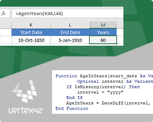
The Excel function DATEDIF(start_date,end_date,»y») is a very simple way to calculate the age of a person if the dates are after 1/1/1900. The VBA date functions like Year(), Month(), Day(), DateSerial(), DateValue() are able to handle all the Gregorian dates, so custom functions based on the VBA functions can allow you to work with dates prior to 1900. The function below is designed to work like DATEDIF(start_date,end_date,»y») as long as end_date >= start_date.
=AgeInYears(start_date,end_date)
Example: =AgeInYears(«10-Oct-1850″,»5-Jan-1910») returns the value 59.
Function AgeInYears(start_date As Variant, end_date As Variant) As Variant
    AgeInYears = Year(end_date) - Year(start_date) - _
    Abs(DateSerial(Year(end_date), Month(start_date), _
    Day(start_date)) > DateValue(end_date))
End Function
More Custom Excel Function Examples
For an excellent explanation of pretty much everything you need to know to create your own custom Excel function, I would recommend Excel 2016 Formulas. The book provides many good user defined function examples, so if you like to learn by example, it is a great resource.
- Rounding Significant Figures in Excel :: Shows how to return #NUM and #N/A error values.
- UDF Examples — www.ozgrid.com — Provides many examples of user defined functions, including random numbers, hyperlinks, count sum, sort by colors, etc.
- Build an Excel Add-In — http://www.fontstuff.com/vba/vbatut03.htm — An excellent tutorial that takes you through building an add-in for a custom excel function.
Note: I originally published most of this article in 2004, but I’ve updated it significantly and included other examples, as well as the download file.