
Format numbers as dates or times
Excel for Microsoft 365 Excel for Microsoft 365 for Mac Excel for the web Excel 2021 Excel 2021 for Mac Excel 2019 Excel 2019 for Mac Excel 2016 Excel 2016 for Mac Excel 2013 Excel 2010 Excel 2007 Excel for Mac 2011 More…Less
When you type a date or time in a cell, it appears in a default date and time format. This default format is based on the regional date and time settings that are specified in Control Panel, and changes when you adjust those settings in Control Panel. You can display numbers in several other date and time formats, most of which are not affected by Control Panel settings.
In this article
-
Display numbers as dates or times
-
Create a custom date or time format
-
Tips for displaying dates or times
Display numbers as dates or times
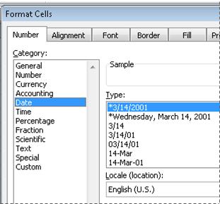
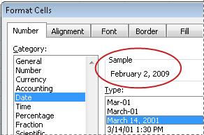
You can format dates and times as you type. For example, if you type 2/2 in a cell, Excel automatically interprets this as a date and displays 2-Feb in the cell. If this isn’t what you want—for example, if you would rather show February 2, 2009 or 2/2/09 in the cell—you can choose a different date format in the Format Cells dialog box, as explained in the following procedure. Similarly, if you type 9:30 a or 9:30 p in a cell, Excel will interpret this as a time and display 9:30 AM or 9:30 PM. Again, you can customize the way the time appears in the Format Cells dialog box.
-
On the Home tab, in the Number group, click the Dialog Box Launcher next to Number.

You can also press CTRL+1 to open the Format Cells dialog box.
-
In the Category list, click Date or Time.
-
In the Type list, click the date or time format that you want to use.
Note: Date and time formats that begin with an asterisk (*) respond to changes in regional date and time settings that are specified in Control Panel. Formats without an asterisk are not affected by Control Panel settings.
-
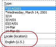
To display dates and times in the format of other languages, click the language setting that you want in the Locale (location) box.
The number in the active cell of the selection on the worksheet appears in the Sample box so that you can preview the number formatting options that you selected.

Top of Page
Create a custom date or time format
-
On the Home tab, click the Dialog Box Launcher next to Number.
You can also press CTRL+1 to open the Format Cells dialog box.
-
In the Category box, click Date or Time, and then choose the number format that is closest in style to the one you want to create. (When creating custom number formats, it’s easier to start from an existing format than it is to start from scratch.)
-
In the Category box, click Custom. In the Type box, you should see the format code matching the date or time format you selected in the step 3. The built-in date or time format can’t be changed or deleted, so don’t worry about overwriting it.
-
In the Type box, make the necessary changes to the format. You can use any of the codes in the following tables:
Days, months, and years
|
To display |
Use this code |
|---|---|
|
Months as 1–12 |
m |
|
Months as 01–12 |
mm |
|
Months as Jan–Dec |
mmm |
|
Months as January–December |
mmmm |
|
Months as the first letter of the month |
mmmmm |
|
Days as 1–31 |
d |
|
Days as 01–31 |
dd |
|
Days as Sun–Sat |
ddd |
|
Days as Sunday–Saturday |
dddd |
|
Years as 00–99 |
yy |
|
Years as 1900–9999 |
yyyy |
If you use «m» immediately after the «h» or «hh» code or immediately before the «ss» code, Excel displays minutes instead of the month.
Hours, minutes, and seconds
|
To display |
Use this code |
|---|---|
|
Hours as 0–23 |
h |
|
Hours as 00–23 |
hh |
|
Minutes as 0–59 |
m |
|
Minutes as 00–59 |
mm |
|
Seconds as 0–59 |
s |
|
Seconds as 00–59 |
ss |
|
Hours as 4 AM |
h AM/PM |
|
Time as 4:36 PM |
h:mm AM/PM |
|
Time as 4:36:03 P |
h:mm:ss A/P |
|
Elapsed time in hours; for example, 25.02 |
[h]:mm |
|
Elapsed time in minutes; for example, 63:46 |
[mm]:ss |
|
Elapsed time in seconds |
[ss] |
|
Fractions of a second |
h:mm:ss.00 |
AM and PM If the format contains an AM or PM, the hour is based on the 12-hour clock, where «AM» or «A» indicates times from midnight until noon and «PM» or «P» indicates times from noon until midnight. Otherwise, the hour is based on the 24-hour clock. The «m» or «mm» code must appear immediately after the «h» or «hh» code or immediately before the «ss» code; otherwise, Excel displays the month instead of minutes.
Creating custom number formats can be tricky if you haven’t done it before. For more information about how to create custom number formats, see Create or delete a custom number format.
Top of Page
Tips for displaying dates or times
-
To quickly use the default date or time format, click the cell that contains the date or time, and then press CTRL+SHIFT+# or CTRL+SHIFT+@.
-
If a cell displays ##### after you apply date or time formatting to it, the cell probably isn’t wide enough to display the data. To expand the column width, double-click the right boundary of the column containing the cells. This automatically resizes the column to fit the number. You can also drag the right boundary until the columns are the size you want.
-
When you try to undo a date or time format by selecting General in the Category list, Excel displays a number code. When you enter a date or time again, Excel displays the default date or time format. To enter a specific date or time format, such as January 2010, you can format it as text by selecting Text in the Category list.
-
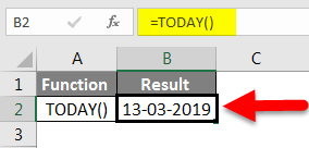
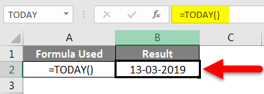
To quickly enter the current date in your worksheet, select any empty cell, and then press CTRL+; (semicolon), and then press ENTER, if necessary. To insert a date that will update to the current date each time you reopen a worksheet or recalculate a formula, type =TODAY() in an empty cell, and then press ENTER.
Need more help?
You can always ask an expert in the Excel Tech Community or get support in the Answers community.
Need more help?
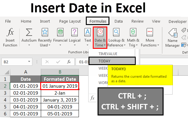
In Microsoft Excel, the date can be inserted in a variety of ways, including using a built-in function formula or manually entering the date, such as 22/03/2021, 22-Mar-21, 22-Mar, or March 22, 2021. These date functions are typically used for cash flows in accounting and financial analysis.
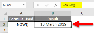
In Excel, there is a built-in function called TODAY() that will insert the exact today’s date and will give the updated date whenever the workbook is opened. The NOW() built-in function can also be used to insert the current date and time, and this function will be kept up to date if we open the workbook multiple times.
Inserting the date:
In the Formula tab, the built-in TODAY is categorized under the DATE/TIME function.
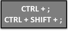
Alternate to insert the date in Excel the below keyboard shortcut can be used:
CTRL+;
It will insert the current date.
To insert the current date and time we can use the following shortcut keys:
CTRL+; <space key> CTRL+SHIFT+;
It returns the current date and time to us.
1. Inserting specific date in Excel:
We have to use DATE() to insert a specific valid date in Excel. We can notice in the above function that the DATE requests to provide Year, Month, Day values. If we provide the details, the default date will be shown as below:
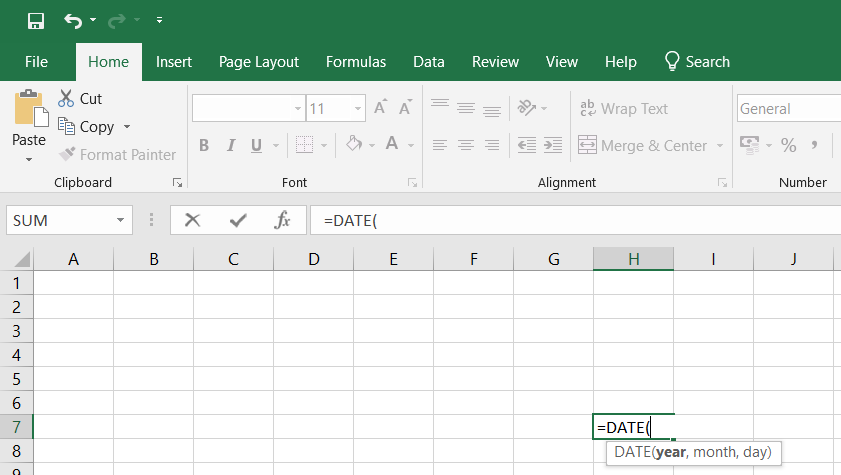
Image 1.1
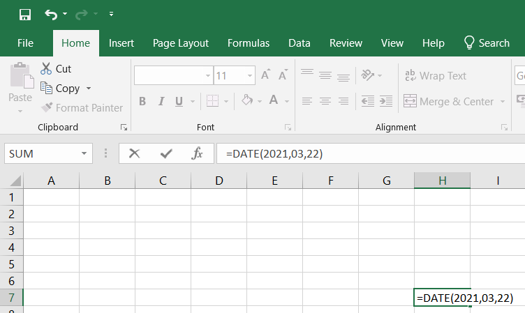
Image 1.2
2. Inserting static date and time:
A static value in a sheet does not change if the sheet is recalculated or opened. To do so follow the below steps:
Step 1: Select the cell in which the current date or time will be inserted on a table.
Step 2: Do one of the next:
- Press Ctrl+;(semi-colon) to insert your current date.
- Press the Ctrl+Shift+;(semi-colon) to insert the current time.
- Press Ctrl+;(semi-column) to insert the current date and time then press Space, and press Ctrl+Shift+; (semi-colon).
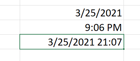
Static date and time
3. Inserting a date in Excel via a drop-down calendar:
It may be a good idea to include a down calendar in your worksheet if you set up a table for other users and want to make sure that the dates enter correctly. You can fill in the dates with a mouse click and be 100% confident that all dates are entered in a suitable format. You can use Microsoft Date Picker control when you use a 32-bit version of Excel. Microsoft Date Picker Control will not work when you are using a 64-bit Excel 2016, Excel 2013 version.
4. Inserting an automatically updatable today’s date and current time:
If you want to keep your Excel date up-to-date today, use one of the following Excel date functions:
=TODAY() -> inserts in a cell the current date.
=NOW() -> inserts in a cell the current and current date.
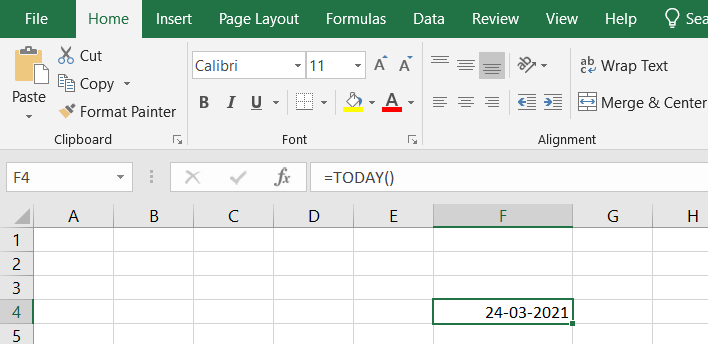
=TODAY example
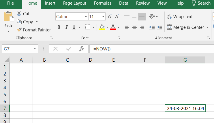
=NOW example
Please remember that when using the Excel date functions:
- The date and the time returned will not be refreshed on an ongoing basis, but only when the chain is reopened or re-calculated.
- The functions take the current system clock date and time.
5. Auto-populate dates in Excel
To autofill a series of dates in which one day is incremented, you can use the Excel AutoFill function. It is a common way to automatically fill a column or row. To do so follow the below steps:
- Enter the original date in the first cell.
- Click the first date on your cell and then drag the fill handle to or from the cells you want Excel to add dates.
Autofill weekdays, months, or years:
There are two ways of automatically adding weekdays, months, or years to the selected range of cells. To so follow the below steps:
- You can use the above-mentioned Excel AutoFill options. Click the AutoFill Options icon and choose the option you want when the range is populated by sequential dates.
- Another way to enter your first date will be to right-click the fill handle and drag and release the fill handle through the cells you automatically want to fill with dates. Excel displays a context menu and selects the appropriate option.
Auto-populate dates
See all How-To Articles
This tutorial covers how to insert dates in Excel.
The Date Format
Like numbers, currency, time and others, the date is a quintessential number format in Excel.
Though Excel tries its best to auto-recognize data types, it doesn’t always succeed. To manually apply the date format to a cell or group of cells, select the HOME menu, expand the Number dropdown and choose short or long date.
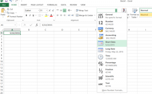
The difference between short and long date formats is that the latter includes the weekday.
Warning! Applying the date format to inappropriate data will give unexpected results!
If you would like to change the default format of the date, with the order of month, day and year, select “More Number Formats..” under the Number dropdown.

At the bottom of the dropdown, More Number Formats allows you to customize the order of the elements in the date. You can also choose a particular date format based on your location.

Note: The location options must be compatible with the language of your machine.
Today’s Date
To insert today’s date, there are two primary functions: NOW() and TODAY(). The former also includes the current time.

To change the order of the resulting date, follow the steps mentioned earlier to customize the format.
Shortcut: You can also use shortcut “CTRL + ; “ for TODAY() and “CTRL + SHIFT + ;” for NOW().
Auto Populate Dates
Excel treats dates and numbers in almost the same way. Because dates are implemented as serial numbers, you can perform arithmetic operations with them such as auto-populating.
Just as you would auto-populate cells with numbers, select a cell with a date and drag the fill handle through the cells you want to fill.
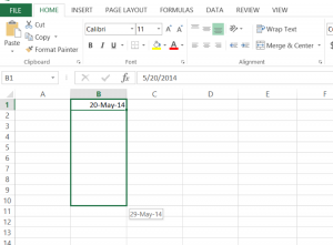
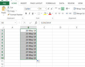
The example demonstrates how to fill cells by day increments, but you can also increment by week, month and year. Just follow the same steps that you would to fill cells by day increments, and then select the icon at the bottom right next to the fill handle. On the dropdown list, choose your increment.


Fill Dates by Custom Interval
You might want to fill dates and increment by an amount other than one unit of time.
To fill cells with dates by every N number of days, first perform the steps as you would to autofill dates normally. Then in the editing section of the HOME menu, click Fill then Series.

In the dialog box, select “Linear” and under “Step value”, provide the desired increment.

Result: The dates will be auto filled every three days.

Create a Date from Separate Columns
If you happen to work with Excel data where the year, month and day are in separate columns, you can use the DATE function to merge them into one date.
DATE(YEAR, MONTH, DAY)

Note: Months have to be in numeric form.
-
1
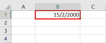
Type the desired date into a cell. Double-click the cell in which you want to type the date, and then enter the date using any recognizable date format. You can enter the date in a variety of different formats.[1]
- Using January 3 as an example, some recognizable formats are «Jan 03,» «January 3», «1/3,» and «01-3.»
-
2
Press the ↵ Enter key. As long as Excel recognizes the date format, it will re-format the cell as a date, which is usually mm/dd/yyyy or dd/mm/yyyy, depending on your locale.
- If the text automatically aligned to the right, then Excel recognized it as a date and re-formatted it.
- If the text stayed aligned to the left, Excel is treating the input as text rather than a date. This could be because it cannot recognize your input as a date, or because that cell’s format is set to something besides a date.
Advertisement
-
3
Right-click the date cell and select Format Cells. A new window will pop up.
-
4
Click the Number tab. It’s the first tab.
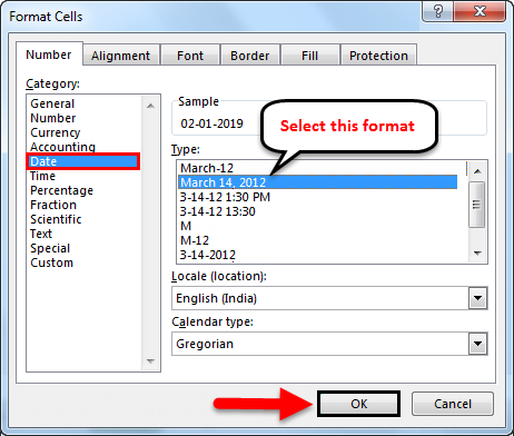
-
5
Select Date in the «Category» panel. A variety of date formats will appear on the right side of the window.
-
6
Select your desired date format under «Type.» This reformats the selected cell to display in this format.
- You can also change your locale to access date formats used in your location.
-
7
Click OK. The selected cell(s) will now display dates in the selected format.


Advertisement

-
1
Click the cell in which you want today’s date to appear. This can be in an existing formula, or in a new cell.
-
2
Type an equal sign = followed by the formula TODAY(). If you wish to retrieve the current time as well, use NOW() instead of TODAY().[2]
-
3
Hit ↵ Enter. Excel will return today’s date as the cell value. This is a dynamic date, meaning it will change depending on when you are viewing the sheet.
- Use the shortcuts Ctrl + ; and Ctrl + Shift + ; instead to set a cell’s value to today’s date and time respectively as a static value. These values will not update, and act as a timestamp.


Advertisement
-
1
Click the cell in which you want to type the date.
-
2
Type an equal sign = followed by the date formula DATE(year, month, day). Year, month, and day should be numerical inputs.
-
3
Hit ↵ Enter. Excel will return the default date format, which is usually mm/dd/yyyy or dd/mm/yyyy depending on your locale.
-
4
Expand on the formula if required. You can set formulas for the year, month, and day values. Or, you can use the DATE function within other formulas.
- For instance, DATE(2010,MONTH(TODAY()),DAY(TODAY())) sets the cell’s value as today’s month and day in 2010. The formula DATE(2020,1,1)-10 sets the value to 10 days before 1/1/2020.


Advertisement
-
1
Type the desired date into a cell. Double-click the cell in which you want to type the date, and then enter the date using any recognizable date format. You can enter the date in a variety of different formats.
- Using January 3 as an example, some recognizable formats are «Jan 03,» «January 3», «1/3,» and «01-3.»
-
2
Hit ↵ Enter. Excel will re-format the cell and align the text to the right if it has recognized it as a date.
-
3
Select all the cells you wish to fill with dates. Include the cell in which you just entered the date. To select, drag your mouse over all the cells, select an entire column or row, or hold Ctrl (PC) or ⌘ Cmd (Mac) while clicking each cell.
-
4
Click Fill on the Home tab. It’s at the top of Excel in the «Editing» section and looks like a white box with a blue down arrow.
-
5
Click Series…. It is near the bottom.
-
6
Select a «Date unit.» Excel will use this to fill the blank cells based on this setting.
- For instance, if you select «Weekday,» all the blank cells will populate with the weekdays following the initial input date.
-
7
Click OK. Make sure the are dates filled in correctly.


Advertisement
Ask a Question
200 characters left
Include your email address to get a message when this question is answered.
Submit
Advertisement
-
Set a custom date format in Excel by right-clicking a cell, clicking Format Cells, and selecting «Custom» as the category in the Number tab. Review the available date options. Create your own by typing the format code using an existing code.
Advertisement
References
About This Article
Article SummaryX
1. Click on a cell.
2. Type in a date.
3. Hit Enter.
4. Review the date format. Change by right-clicking and selecting Format Cells.
Did this summary help you?
Thanks to all authors for creating a page that has been read 12,957 times.
Is this article up to date?
What is a date in Excel?
A date is a number! And like any number (currency, percentage, decimal, …), you can customize your date format 👍
Dates are whole numbers
Usually, when you insert a date in a cell it is displayed in the format dd/mm/yyyy or mm/dd/yyyy.
Let’s say you have the date 01/01/2016 in a cell. If you change the cell’s format to Standard, the cell displays 42370 😕🤔

Explanation of the numbering
In Excel, a date is the number of days since 01/01/1900 (the first date in Excel).
So 42370 is the number of days between 01/01/1900 and 01/01/2016.
Date format
Dates can be displayed in different ways using the following 2 options (available in the Number Format dropdown in the main menu):
- Short Date
- Long Date

How to customize a date?
To customize a date:
- Open the dialog box Custom Number (with the shortcut Ctrl + 1 or by clicking on the menu More number formats at the bottom of the number format dropdown)

- In this dialog box, you select ‘Custom‘ in the Category list and write the date format code in ‘Type‘.

To format a date, you just write the parameter d, m or y a different number of times. For example,
- dd/mm/yyyy will display 01/01/2016
- dd mmm yyyy => 01 Jan 2016
- mmmm yyyy => January 2016
- dddd dd => Friday 01
In function of your language , the letter could be different:
- t for «tag» (day) in German
- j for «jour» (day) in French
- a for «año» (year) in Spanish
Don’t write text in your cell !!!
With dates, one of the most common mistakes is to write text inside the format code (1 January 2016 for example). Never do this in Excel ⛔⛔⛔
If you do this, the contents of the cell will be Text and not a number
- In Excel, text is always displayed on the left of a cell.
- A number or a date is displayed on the right.

If you want to display the month in letters, just change the month format of your date.
Different examples of custom date
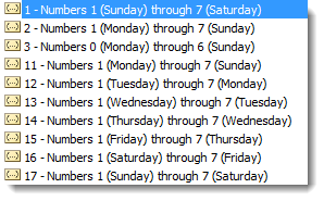
The following document shows you the same date but in different formats. The code for each date is in column A.

Different writing of dates according to the format code
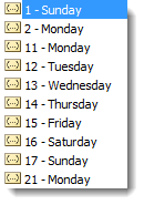
In the following document, you can see the impact of each format on the same date.

Excel Insert Date (Table of Contents)
- Insert Date in Excel
- How to Insert Date in Excel?
Insert Date in Excel
In Microsoft Excel, we can insert the date in various ways either by using built-in function formula or by inserting the date manually like 1/02/2019, or 01-Feb-19, or 01-Feb, or February 1, 2019. These date functions are normally used in accounting and financial analysis for cash flows.
In Excel, for inserting the date, we have a built-in function called TODAY () which will insert the exact today’s date, and this function will give you the updated date whenever we open the workbook. We can also use the NOW () built-in function, which inserts the current date and time, and this function also will be kept on getting updated when we open the workbook for multiple times.
How to Insert?
TODAY built-in function is categorized under the DATE/TIME function in the Formula tab.
We can use the alternative ways to insert the date in excel by using the keyboard shortcut key listed below.
- CTRL+; (Semicolon), which will insert the current date.

To insert the current date and time we can use the below shortcut key as follows.
- CTRL+; and then CTRL+SHIFT+; which will give us the current date and time.
Let’s understand How to Insert Date in Excel by different methods along with some examples.
Insert Date in Excel – Example #1
Insert date automatically in Excel Using TODAY Function:
You can download this Insert Date Excel Template here – Insert Date Excel Template
In this example, we will see how to automatically insert the date using the TODAY built-in function by following the below steps.
Step 1 – Open a new workbook.
Step 2 – Go to the Formulas tab.
Step 3 – Select the DATE & TIME so that we will get the list of function as shown below.
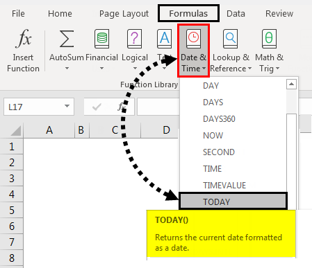
Step 4 – Select the TODAY function.
Step 5 – Once we click on the today function, we will get the dialog box for Function Arguments. Then Click on OK.
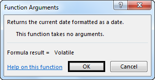
Excel will insert the current data as shown below.
Step 6 – We can type the function directly as TODAY, then press the Enter key to get the current date in the sheet, shown below.
Alternatively, we can also use the shortcut key for inserting the date as CTRL + ;
Insert Date in Excel – Example #2
Insert date automatically in Excel Using NOW Function:
In this example, we will see how to use the NOW function to insert date in excel by following the below steps.
Step 1 – First, open a new sheet.
Step 2 – Type =NOW() function in the worksheet. Then press the Enter key so that we will get the current date and time as shown below.

Step 3 – We can format the date and time by right-clicking the cells to get the format cells to the option shown below.
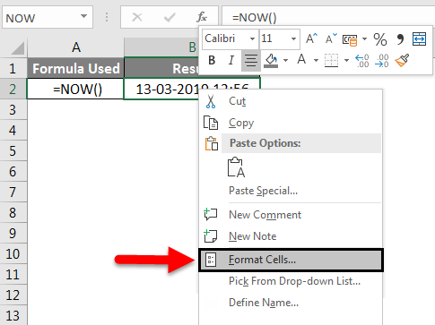
Step 4 – Once we click on the Format Cells we will get the below dialog box. Then choose the desired format that we need to display here in this example.
We will choose the date format of the second option, i.e. Date/Month/Year, as shown below.
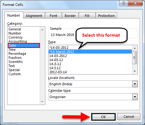
Step 5 – Click OK so that we will get the date in the desired format, as shown below.
Insert Date in Excel – Example #3
Manually Insert a date in Excel:
In this example, we will learn how to insert date manually with the below example
In excel if we enter the normal data by default, Excel will convert the number to date format, in rare cases if we import the sheet from other sources excel will not recognize the format. In such a case, we need to enter the date manually and change it to date format.
Follow the below steps to insert the date
Step 1 – Open a new workbook.
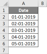
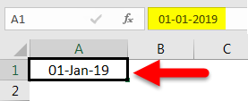
Step 2 – Insert the various date manually as 01-01-19, 01-02-19,03-03-19, which is shown below.
Step 3 – We can change the date format by selecting the format option which is shown below.
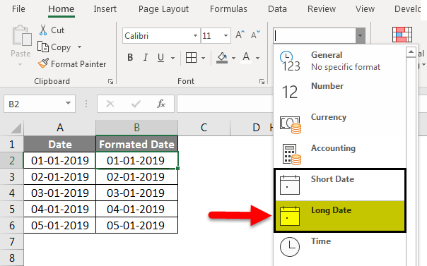
In the above screenshot, we can see the date format as Short Date and Long Date.
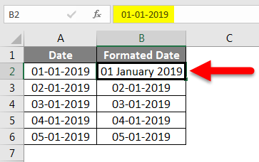
Step 4 – Click on the Long Date so that we will get the date in the desired format, as shown below.
We can insert the date in various formats by formatting the date as follows
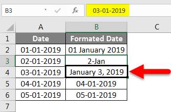
Step 5 – Click on cell B3 and right-click on the cell to get the format cells to the option shown below.
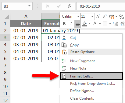
Step 6 – Click on the format cells so that we will get the format option dialog box which is shown below.
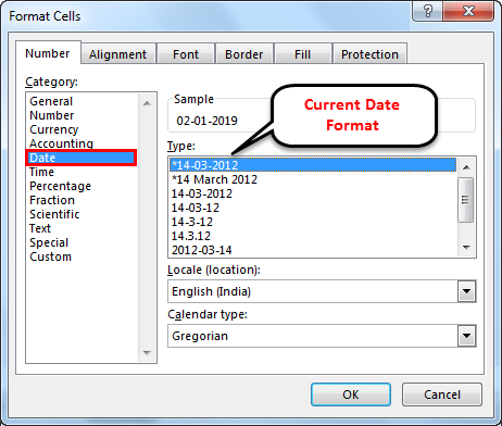
The above format option by default excel will show the * (Asterisk)mark, which means the current date format.
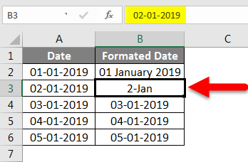
Step 7 – Select the other date format as 14-Mar, which means Date- Month, which is shown below.
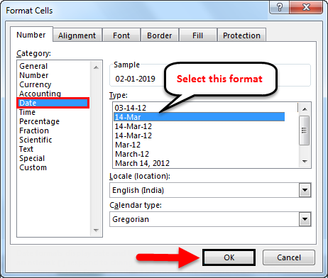
Step 8 – Now click OK so that we will get the desired date output as follows.
We can change the third date also in a different date format by applying the formatting option as above where we have selected the below option as Month, Date, Year.
Step 9 – Click OK so that we will get the final output which is shown below.
In the below screenshot, we have inserted the date in a different format using the formatting option.
Insert Date in Excel – Example #4
Insert dates automatically by dragging the cells:
In excel, we can simply insert the date and drag the cell automatically by following the below steps.
Step 1 – Open a new workbook and Type the date as 01-Jan-19, which is shown below.
Step 2 – Now drag down the cells using the mouse as shown below.
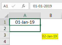
Once we drag down the mouse, Excel will display the auto-increment date in the below cell.
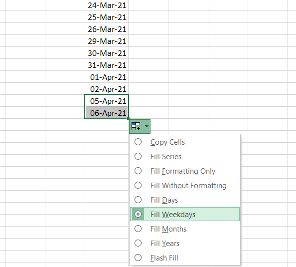
Step 3 – Drag down the cells up to 05-Jan-19, as shown below.
We have inserted the date by just dragging the cells and we can notice that there is a + (Plus) sign symbol which allows us to auto-fill the date.
Once we click on the + sign symbol, we will get the below options like Fill Days. Fill Weekdays, Fill Months, Fill Years.
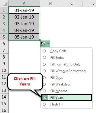
Step 4 – Now, just click on the option Fill years so that excel will insert the years automatically, as shown below.
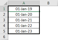
Now we can see the difference that auto-fill has changed the date by incrementing only the years and keeping them all the date as a common number.
Things to Remember
- We have to be very careful if we use TODAY built-in function in excel because today function will always return the current date, for example, if we apply the today function in the report yesterday and if you try to open the same report we will not get yesterday’s date and today function will update only the current date.
- We can insert the date using auto-fill options but make sure that we are inserting correct dates in the excel because autofill will change the date for the entire cell.
Recommended Articles
This has been a guide to Insert Date in Excel. Here we discussed Insert Date in Excel and How to Insert Date using different methods in Excel along with practical examples and downloadable excel template. You can also go through our other suggested articles–
- Insert Calendar In Excel
- Date Formula in Excel
- EDATE Excel Function
- Excel Add Months to Dates
In Excel, every valid date is stored as a form of the number. One important thing to be aware of in Excel is that we have a cut-off date of “31-Dec-1899”. Therefore, every date we insert in Excel will be counted from “01-Jan-1900 (including this date)” and stored as a number.
Table of contents
- How to Insert Date in Excel?
- Examples
- Example #1 – Date Stored as a Number
- Example #2 – Inserting Specific Date in Excel
- Example #3 – Changing the Inserted Date Format in Excel
- Example #4 – Insert List of Sequential Dates in Excel?
- Example #5 – Insert Dates with NOW() and TODAY() Excel Function
- Example #6 – How to Extract Selective Information from the Inserted Excel Date Values.
- Example #7 – Using TEXT() for Inserting Dates in Excel
- How to Change the Format of the Inserted Date in Excel?
- Things to Remember
- Recommended Articles
- Examples
Examples
Here, we will learn how to insert a date in Excel with the help of the examples below.
Example #1 – Date Stored as a Number
In the Excel sheet, let us take 50, 100, and today’s date, 30/01/2019.

Now, we can observe how data is stored in Excel when we change the formatting of the above data to date and accounting format.
50 – Change format to short date
100 – Change format to short date
30/01/2019 – Change format to accounting as it already in date format
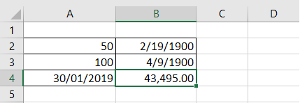
If we observe the number 50 has been changed to date. It displayed exactly 50 days from 01/01/1900 (including this date in the count). Similarly, for the number 100, the date indicated in the exact count from 01/01/1900. And the third observation, which is already in date format and we changed to number format, displays “43,495.” So, today, 30/01/2019 is 43,495 days away from the cut-off date.
Example #2 – Inserting Specific Date in Excel
To insert a specific valid date in Excel, we must use DATE()The date function in excel is a date and time function representing the number provided as arguments in a date and time code. The result displayed is in date format, but the arguments are supplied as integers.read more.
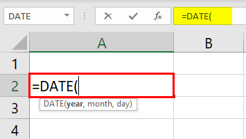
In the above function, we can observe that DATE asks to provide “year,” “month,” and “day” values. As we give the details of it, then this displays the date in default format as below:
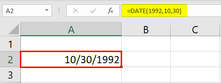
In the above example, we had given the “year” as 1992, “month” as 10, and “day” as 30. But, the output is displayed as per the default format.
Example #3 – Changing the Inserted Date Format in Excel
As seen in our earlier examples, we have displayed the date in a pre-defined format. To change the date format, we should go to “Format Cells.” Let us see how we can do it:
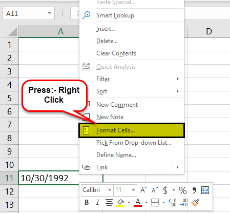
To access the “Format Cells,” we should right-click on the “Date” cell. Then, the above list of operations will pop out. Here, we must select the “Format Cells,” which may take us to the “Format Cells” window.
We got the list in a different format for the date as above. So, let us select one of the formats and see how the format got changed as below.

It is an important formatting feature that helps select dates as per their required format for different organizations.
Example #4 – Insert List of Sequential Dates in Excel?
If we want to list out of the sequential dates, we can select the start date, dragging it down until we reach the end date as per your requirement.
We must insert the date manually (do not use DATE()).
And drag it down as below.
Here we got the list of dates in a sequence from the starting date.
Example #5 – Insert Dates with NOW() and TODAY() Excel Function
To get the present-day date, we can use TODAY()Today function is a date and time function that is used to find out the current system date and time in excel. This function does not take any arguments and auto-updates anytime the worksheet is reopened. This function just reflects the current system date, not the time.read more and get the present day and the current time. Then, we should go with the NOW() FunctionIn an excel worksheet, the NOW function is used to display the current system date and time. The syntax for using this function is quite simple =NOW ().read more. Let us see the example below:

We also got a keyboard shortcut instead of the formulas.
We should use the “Alt +” shortcut instead of the TODAY() Excel function to get the present date.
We should use the “Alt + Shift + ” shortcut instead of the NOW() Excel function to get the present date along with the time.
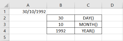
There are three important functions in Excel that help us extract the specific information from the date. They are:
- DAY()In Excel, the DAY function calculates the day value from a given date. This function accepts a date as an argument and returns a two-digit numeric value as an integer value representing the given date’s day. The formula to use this function is =Edate(serial number).read more
- MONTH()The Month Function is a date function that determines the month for a given date in date format. It takes an argument in a date format and displays the result in integer format.read more
- YEAR()The year function in excel is a date function to calculate the year from a given date. This function takes a serial number as an argument and returns a four-digit numeric value representing the year of the given date, formula = year (serial number)read more
Example #7 – Using TEXT() for Inserting Dates in Excel
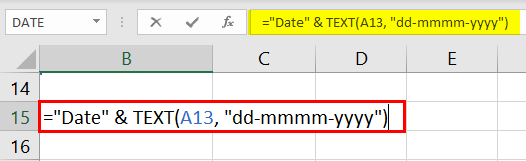
TEXT() is one of the very important formulas for the presentation of data into a certain desired custom format.
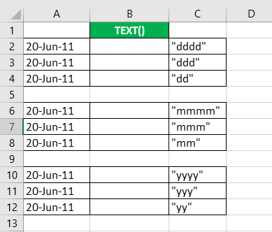
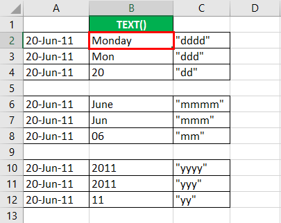
Let us assume the dates as per the above example. We can get the day, month, year, and per the formats mentioned in the third column.
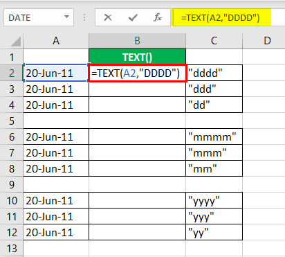
Using the TEXT() as above, we can derive as per the format required.
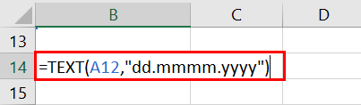
We can also use the TEXT() in changing the date format as per our requirement. We can avoid going to “Format Cells” and changing the format. It will also reduce the time consumption when changing the format.
Let us see how we can change the format using the TEXT().
TEXT() will also help us in concatenating with a dateTo concatenate a date with other values in Excel, we can use the & operator or the built-in concatenate function. For example, if we use =»ABC»&NOW(), the output will be ABC14/09/2019.read more.
However, when we try to concatenate without using the TEXT() then, it may display the number instead of the date as below:
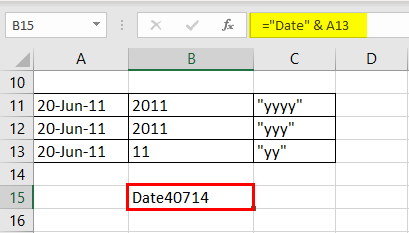
By using the TEXT(), we can concatenate with an actual date as below:
How to Change the Format of the Inserted Date in Excel?
If we observe from the above example, the date is in the form of MM/DD/YYYY. Suppose we want to change the format, then we can do it as per below:
We should go to the “Control Panel” and select ” Ease of Access.” Then, we can visualize the option of the clock, language, and region.
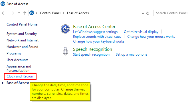
Click on the above option. It will pop out to other windows where we can get a choice of the region and go on that.
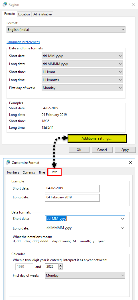
Here, we can select the date format as per our requirement, short date or long date. It will be the default setting of the date once we apply it. If we want to go to the previous format, we can reset it on the window.
Things to Remember
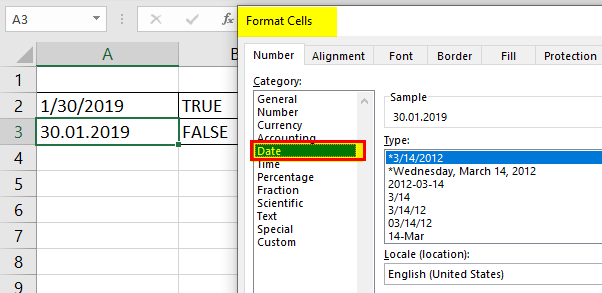
Inserting a valid date in excel should always be stored as a number. We can verify this condition by using ISNUMBER()ISNUMBER function in excel is an information function that checks if the referred cell value is numeric or non-numeric.read more.
Let us take the date in two different formats, as shown above. Inserting a valid date in Excel should always be stored in the number format, so we need to verify the same.
As we check for the number using the ISNUMBER()ISNUMBER function in excel is an information function that checks if the referred cell value is numeric or non-numeric.read more, function, the date which is stored in the form of the number and a valid date will be “TRUE” or else “FALSE.”
In our example above :
- 30/01/2019 – This is TRUE as it is stored in the form of a number, and this date is valid
- 30.01.2019 – This is FALSE, as it is not stored in the form of the number, and it is not valid.
Recommended Articles
This article is a guide to Insert Date in Excel. Here, we discuss how to insert dates in excel along with the top 7 examples using a combination of the DATE(), NOW(), TODAY(), and TEXT() functions. You may also look at these useful functions in Excel: –
- VBA DATEVALUE Function
- EOMONTH Function in Excel
- Date to Text in Excel
- EDATE Function in Excel
 Dates and times are two of the most common data types people work with in Excel, but they are also possibly the most frustrating to work with, especially if you are new to Excel and still learning. This is because Excel uses a serial number to represent the date instead of a proper month, day, or year, nevermind hours, minutes, or seconds. It’s made more complicated by the fact that dates are also days of the week, like Monday or Friday, even though Excel doesn’t explicitly store that information in the cells. Here is the definitive guide to working with dates and times in Excel…
How Excel Stores Dates
The source of most of the confusion around dates and times in Excel comes from the way that the program stores the information. You’d expect it to remember the month, the day, and the year for dates, but that’s not how it works…
Excel stores dates as a serial number that represents the number of days that have taken place since the beginning of the year 1900. This means that January 1, 1900 is really just a 1. January 2, 1900 is 2. By the time we get all the way to the present decade, the numbers have gotten pretty big… September 10, 2013 is stored as 41527.
Importantly, any date before January 1, 1900 is not recognized as a date in Excel. There are no “negative” date serial numbers on the number line.
It seems confusing, but it makes it a lot easier to add, subtract, and count days. A week from September 10, 2013 (September 17, 2013), is just 41527 + 7 days, or 41534.
How Excel Stores Times
Excel stores times using the exact same serial numbering format as with dates. Days start at midnight (12:00am or 0:00 hours). Since each hour is 1/24 of a day, it is represented as that decimal value: 0.041666…
That means that 9:00am (09:00 hours) on September 10, 2013 will be stored as 41527.375.
When a time is specified without a date, Excel stores it as if it occurred on January 0, 1900. In other words, 3:00pm (15:00 hours) is stored as 0.625. This can make doing math for time-only values (that have no date) challenging, since subtracting 6 hours (6:00) from 3:00am (03:00 hours) will become negative and count as an error: 0.125 – 0.25 = -0.125, which is displayed as #########.
Minutes and seconds in Excel work the same way as hours…
A minute is 1/60 of an hour, which is 1/24 of a day, or 1/1440 of a day in total, which calculates to 0.00069444…
A second is 1/60 of an minute, which is 1/60 of an hour, which is 1/24 of a day, or 1/86400 of a day in total, which calculates to 0.00001157407…
Working with Dates and Times
DATE() and TIME()
Serial numbers aren’t all that intuitive to use. Fortunately, Excel has a set of functions to make it easier to find and use dates and times, starting with DATE and TIME. The syntax is as follows:
=DATE(year, month, day)
=TIME(hours, minutes, seconds)
For both functions, specify the year, month, and day, or hours, minutes, and seconds as numbers. For example, September 10, 2013 can be entered as:
=DATE(2013,9,10)
It will be stored as 41527, which means that it is technically storing 12:00am on September 10, 2013.
For times, 6:00pm (18:00 hours) can be entered as:
=TIME(18,0,0)
It will be stored as 0.75, which means that it is technically storing 6:00pm on January 0, 1900.
If we want to represent a specific time and date, we can add the two functions together. For example, 6:00pm (18:00 hours) on September 10, 2013 can be entered as:
=DATE(2013,9,10)+TIME(18,0,0)
It will be calculate as 41527.75, which means Excel is storing exactly the date we want…
Additional Date and Time Setting Functions
Excel has a few additional functions to make declaring dates easier.
TODAY()
The TODAY function always returns the current date’s serial number. The TODAY function is just entered as:
=TODAY()
This article was written at 6:30pm (18:30 hours) on September 24, 2013, and the TODAY function calculated to 41541. That means that it is technically storing 12:00am on September 24, 2013.
NOW()
A similar function called NOW always returns the current date and time’s serial number. The NOW function is just entered as:
=NOW()
Again, at 6:30pm (18:30 hours) on September 24, 2013, the function calculated to 41541.77081333… NOW stores the exact time and date, down to the second.
EDATE() and EOMONTH()
The EDATE function gives the date the specified number of months away from the input date. The EOMONTH function gives the date of the last day of the month. It can do so for the current month or a number of months in the future or the past. The syntax for each is as follows:
=EDATE(start_date, months)
=EOMONTH(start_date, months)
The start_date can be any date-formatted cell reference or date serial number.
The months field can be any number, though only the integer value will be used (e.g. it treats 2.8 as 2).
The EDATE and EOMONTH functions strip the time value from the date. For example, For example, if cell A1 stores September 10, 2013, we can get the value 2 months ahead as follows:
=EDATE(A1,2)
Returns 12:00am (0:00 hours) on November 10, 2013, or 41588. This function works even though the months have different numbers of days (September and November have 30, October has 31).
=EOMONTH(A1,2)
Returns 12:00am (0:00 hours) on November 30, 2013, or 41588. Again, this function works even though the months have different numbers of days.
WORKDAY()
Occasionally, it may be useful to count ahead based on work-days (Monday-Friday) instead of all 7 days of the week… For that, Excel has provided WORKDAY. The syntax for WORKDAY is as follows:
=WORKDAY(start_date, days, [holidays])
The start_date is as above.
The days input is the number of workdays ahead (or behind) of the present day you would like to move.
The [holidays] input is optional, but lets you disqualify specific days (like Thanksgiving or Christmas, for example), which might otherwise fall during the work week. These are date serial numbers provided in an array bounded by brackets: { }. To specify multiple holidays, the dates must be held in cells – it is not possible to put multiple DATE functions in an array.
For example, let’s find the date 6 work days before 6:00pm (18:00 hours) on September 10, 2013 (stored in cell A1). Monday, September 2nd is Labor Day, so let’s include that as a holiday:
=WORKDAY(A1,-6,DATE(2013,9,2))
Returns 12:00am (0:00 hours) on August 30, 2013, or 41516. (Note that the function strips the time portion of the date.)
WORKDAY.INTL() (Excel 2010 and newer)
For newer versions of Excel (2010 and later), there is another version of WORKDAY called WORKDAY.INTL. WORKDAY.INTL works just like WORKDAY, but it adds the ability to customize the definition of the “weekend”. The syntax for WORKDAY.INTL is as follows:
=WORKDAY.INTL(start_date, days, [weekend], [holidays])
The start_date, days, and [holidays] inputs work just like the normal WORKDAY function.
The [weekend] input has the following options:
Retrieving Dates in Excel
DAY(), MONTH(), and YEAR()
Now we know how define dates, but we still need to be able to work with them. Serial numbers don’t make it easy to extract months, years, and days, nevermind hours, minutes, and seconds. That’s why Excel has specific functions for pulling out each of these values. For working with the calendar, there is DAY, MONTH, and YEAR. The syntax is simple:
=DAY(serial_number)
=MONTH(serial_number)
=YEAR(serial_number)
The serial_number in each can be any date-formatted cell reference. For example, if cell A1 stores September 10, 2013, we can use each of the formulas in turn:
=DAY(A1)
Returns 10 as a numeric value.
=MONTH(A1)
Returns 9 as a numeric value.
=YEAR(A1)
Returns 2013 as a numeric value.
We could have also given the direct serial number for September 10, 2013:
=DAY(41527)
Returns 10 as a numeric value.
Retrieving Times in Excel
HOUR(), MINUTE(), and SECOND()
For times, the process is very similar. Excel has function to retrieve the hours, minutes, and seconds from a time stamp, conveniently named HOUR, MINUTE, and SECOND. The syntax is identical:
=HOUR(serial_number)
=MINUTE(serial_number)
=SECOND(serial_number)
The serial_number in each can be any time/date-formatted cell reference. For example, if A1 stores 6:15:30pm (18:15 hours, 30 seconds) on September 10, 2013, we can use each of the formulas in turn:
=HOUR(A1)
Returns 18 as a numeric value.
=MINUTE(A1)
Returns 15 as a numeric value.
=SECOND(A1)
Returns 30 as a numeric value.
We could have also given the direct serial number for 6:15:30pm (18:15 hours, 30 seconds) on September 10, 2013:
=SECOND(41527.7607638889)
Returns 30 as a numeric value.
Additional Date Retrieving Functions
WEEKDAY() and WEEKNUM()
Dates don’t just have month and year information. They also encode indirect information… September 10, 2013 happens to also be a Tuesday. Excel has a few of functions to work with the week aspect of dates: WEEKDAY and WEEKNUM. The syntax is as follows:
=WEEKDAY(serial_number, [return_type])
=WEEKNUM(serial_number, [return_type])
The serial_number in each can be any date-formatted cell reference. Since [return_type] is optional, each function assumes that each week starts on Sunday. If cell A1 stores September 10, 2013 (a Tuesday), we can use each of the formulas in turn:
=WEEKDAY(A1)
Returns 3, since Tuesday is the 3rd day of a week that starts on Sunday.
=WEEKNUM(A1)
Returns 37, since September 10, 2013 is in the 37th week of 2013, when you start counting weeks from Sunday.
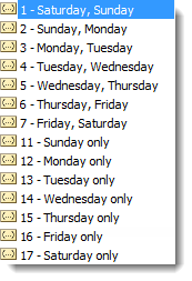
The [return_type] allows you to specify a different default week arrangement. You could let the week start on Monday and run until Sunday, or Saturday until Friday, for example. Excel is annoying, however, and makes the entry different for WEEKDAY and WEEKNUM. The full list of options for WEEKDAY is as follows:
Options 2 and 11 are functionally the same – the first is just there for backwards compatibility with earlier versions of Excel.
The full list of options for WEEKNUM is as follows:
Counting and Tracking Dates
Dates can be added and subtracted like normal numbers because they’re stored as serial numbers. That lets you count the days between two different dates. Sometimes, though, you need to count by a different metric.
NETWORKDAYS()
Above, we learned about WORKDAY, which lets you move back and forth a set number of workdays, ignoring weekends and holidays. But what if you need to measure the number of workdays between two dates? For that, Excel provides NETWORKDAYS. The formula syntax is as follows:
=NETWORKDAYS(start_date, end_date, [holidays])
The start_date and end_date can be any date-formatted cell reference.
The [holidays] input is optional, but lets you disqualify specific days (like Thanksgiving or Christmas, for example), which might otherwise fall during the work week. These are date serial numbers provided in an array bounded by brackets: { }. To specify multiple holidays, the dates must be held in cells – it is not possible to put multiple DATE functions in an array.
For example, if A1 contains 6:00pm (18:00 hours) on September 10, 2013 and B1 contains 9:00am (9:00 hours) on December 2, 2013, we can use NETWORKDAYS to find the number of workdays between the two dates.
Let’s exclude Columbus Day (October 14, 2013), Veterans Day (November 11, 2013), and Thanksgiving Day (November 28, 2013) as holidays. To do so, we have to store those dates in other cells. Let’s put them in C1, C2, and C3:
=DATE(2013,10,14)
=DATE(2013,11,11)
=DATE(2013,11,28)
Now, we can combine them in the function:
=NETWORKDAYS(A1,B1,C1:C3)
The function returns 57 as a numeric value.
NETWORKDAYS.INTL() (Excel 2010 and newer)
For newer versions of Excel (2010 and later), there is another version of NETWORKDAYS called NETWORKDAYS.INTL. NETWORKDAYS.INTL works just like NETWORKDAYS, but it adds the ability to customize the definition of the “weekend”. The syntax for NETWORKDAYS.INTL is as follows:
=NETWORKDAYS.INTL(start_date, end_date, [weekend], [holidays])
The start_date, end_date, and [holidays] inputs work just like the normal WORKDAY function.
The [weekend] input has the following options:
YEARFRAC()
Sometimes it’s useful to measure how much time has passed in years, but subtracting the YEAR function will only round down to the nearest full year. YEARFRAC takes two dates and provides the portion of the year between them. The syntax is as follows:
=YEARFRAC(start_date, end_date, [basis])
The start_date and end_date can be any date-formatted cell reference.
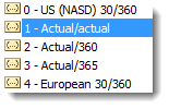
The [basis] input is optional, but lets you specify the “rules” for measuring the difference. Most of the time, you’ll want to use option 1, but here is the full list:
 For example, if A1 contains September 10, 2013 and B1 contains December 2, 2013, we can use YEARFRAC to find the decimal portion of a year between the two dates:
=YEARFRAC(A1,B1,1)
Returns 0.227397260273973.
DATEDIF() (Undocumented Function)
The YEARFRAC function gives you the difference between dates as a fraction of a year, but sometimes you need more control. There is a powerful hidden function in Excel called DATEDIF that can do much more. It can tell you the number of years, months, or days between two dates. It can also track based on only partial inputs, ignoring years or months when calculating days. The syntax for DATEDIF is as follows:
=DATEDIF(start_date, end_date, unit)
The start_date and end_date can be any date-formatted cell reference.
The unit input asks you to specify a string that represents the type of output you want. This is slightly cumbersome, since you must wrap the input in quotes (” “).
For example, if A1 contains September 10, 2012 and B1 contains December 2, 2013, we can use DATEDIF to find the number of full years between the two dates:
=DATEDIF(A1,B1,"Y")
Returns 1 as a numeric value.
Using the same start_date and end_date inputs, here are the output possibilities for DATEDIF using different unit parameters:
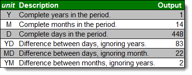
Every time, the unit must be put in quotes (e.g. “Y” or “MD”).
Converting Dates and Times from Text
DATEVALUE() and TIMEVALUE()
All of the above functions work perfectly with date-formatted serial numbers in Excel. Unfortunately, dates and times are often imported into worksheets as text. Most of the assorted functions like MONTH and HOUR are reasonably intelligent about converting on the fly. Occasionally it’s useful to build a date value through concatenation. The two functions Excel provides for this purpose are DATEVALUE and TIMEVALUE. The syntax for each is as follows:
=DATEVALUE(date_text)
=TIMEVALUE(time_text)
The date_text and time_text accept any text string that looks like a date or time.
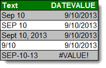
This is how DATEVALUE responds to various date_text inputs:
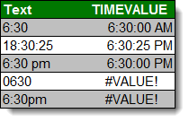
This is how TIMEVALUE responds to various time_text inputs:
Converting Dates and Times to Text
TEXT()
Getting data converted to dates and times is great, but you may also need to get it back out. Sometimes, you need a special format. Other times, you need to look for a date in a text string, and have to match using string tools like FIND and SEARCH. There is one master function for converting dates and times to text strings in Excel, called TEXT. The syntax for TEXT is as follows:
=TEXT(value, format_text)
The value can be any date or time-formatted cell reference.
The format_text input has a large number of options, summarized here:
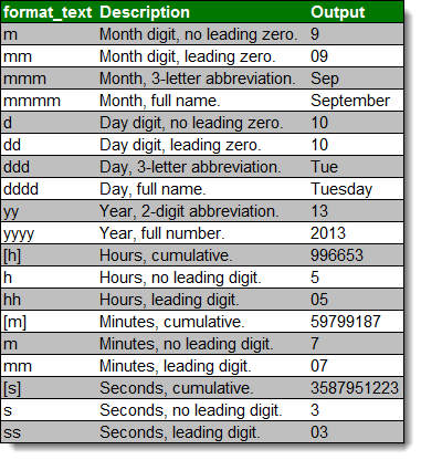
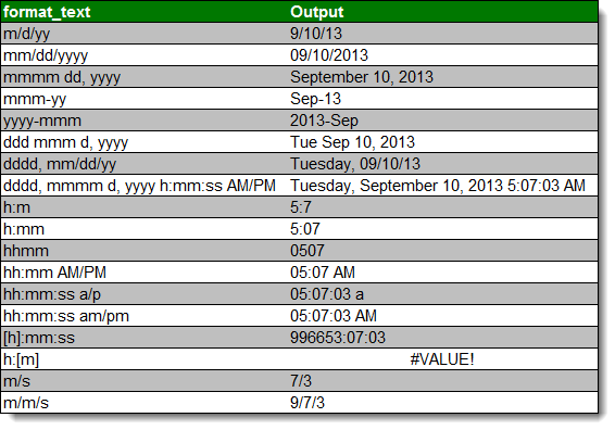
The outputs can be combined with simple formatting characters to produce standard date formats. Using the date 5:07:03am (05:07 hours, 3 seconds) on September 10, 2013, here are examples of possible outputs:
A Common Problem
One issue people frequently run into is that Excel occasionally misinterprets text fields as dates. An example is here:
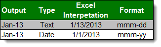
Be careful when entering dates, especially if you are importing from other data sources, to make sure that your “Jan-13” is being stored as January 1, 2013 and not January 13, 2013!
Get the latest Excel tips and tricks by joining the newsletter!
 Andrew Roberts has been solving business problems with Microsoft Excel for over a decade. Excel Tactics is dedicated to helping you master it.
Join the newsletter to stay on top of the latest articles. Sign up and you’ll get a free guide with 10 time-saving keyboard shortcuts!
Other posts in this series…
Bottom line: With Valentine’s Day rapidly approaching I thought it would be good to explain how you can get a date with your Excel skills. Just kidding! 🙂 This post and video explain how the date calendar system works in Excel.
Skill level: Beginner
Dates in Excel can be just as complicated as your date for Valentine’s Day. We are going to stick with dates in Excel for this article because I’m not qualified to give any other type of dating advice. 🙂
Video Tutorial on How Dates Work in Excel
The following is a video from The Ultimate Lookup Formulas Course on how the date system works in Excel.
Watch the Video on YouTube
There are over 100 short videos just like the one above included in the Ultimate Lookup Formulas Course.
This course has been designed to help you master Excel’s most important functions and formulas in an easy step-by-step manner.
The Ultimate Lookup Formulas course is now part of our comprehensive Elevate Excel Training Program.
Click Here to Learn More About Elevate Excel
What is a Date in Excel?
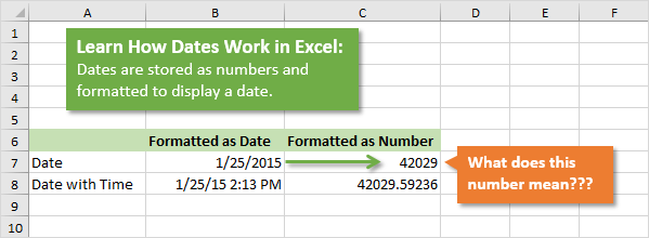
I should first make it clear that I am referring to a date that is stored in a cell.
The dates in Excel are actually stored as numbers, and then formatted to display the date. The default date format for US dates is “m/d/yyyy” (1/27/2016).
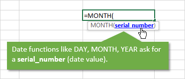
The dates are referred to as serial numbers in Excel. You will see this in some of the date functions like DAY(), MONTH(), YEAR(), etc.
So then, what is a serial number? Well let’s start from the beginning.
The date calendar in Excel starts on January 1st, 1900. As far as Excel is concerned this day starts the beginning of time.
Each Day is a Whole Number
Each day is represented by one whole number in Excel. Type a 1 in any cell and then format it as a date. You will get 1/1/1900. The first day of the calendar system.
Type a 2 in a cell and format it as a date. You will get 1/2/1900, or January 2nd. This means that one whole day is represented by one whole number is Excel.
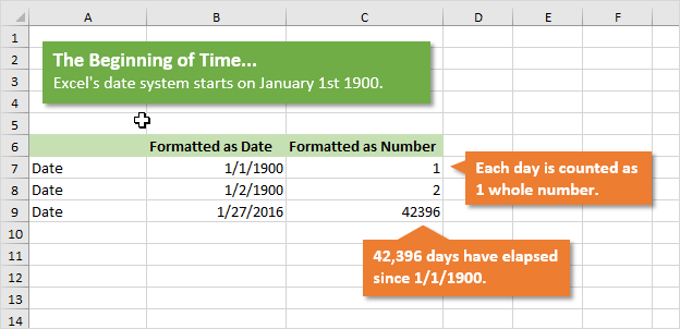
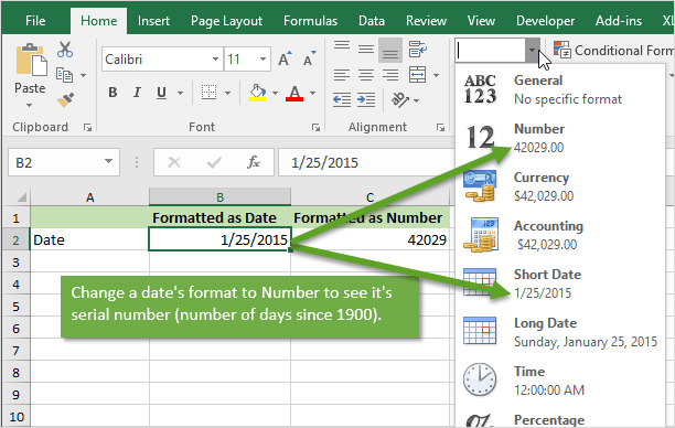
You can also take a cell that contains a date and format it as a number.
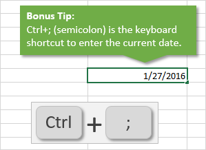
For example, this post was published on 1/27/2016. Put that number in a cell (the keyboard shortcut to enter today’s date is Ctrl+;), and then format it as a number or General.
You will see the number 42,396. This is the number of days that have elapsed since 1/1/1900.
Date Based Calculations
It is important to know that dates are stored as the number of days that have elapsed since the beginning of Excel’s calendar system (1/1/1900).
When you calculate the difference between two dates by subtraction, the result will be the number of days between the two dates.
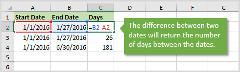
1/27/2016 – 1/1/2016 = 26 days
6/30/2016 – 1/1/2016 = 181 days
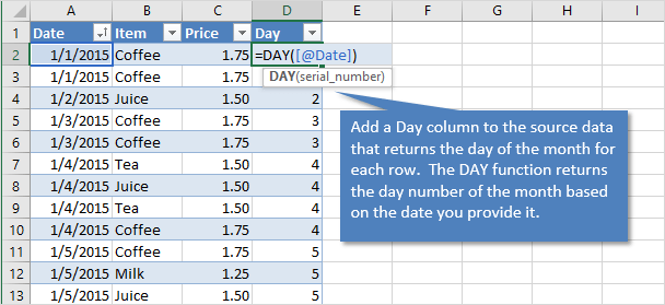
There are a lot of Date functions in Excel that can help with these calculations. Last week we learned about the DAY function for month-to-date calculations with pivot tables.
We won’t go into all the date functions here, but understanding that the serial number represents one day will give you a good foundation for working with dates.
What About Dates with Times?
Do you ever work with dates that contain time values?
These dates are still stored as serial numbers in Excel. When you convert the date with a time to the number format, you will see a decimal number.
This decimal is a fraction of the day.
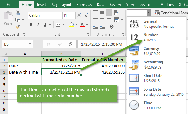
One hour in Excel is represented by the number: 1/24 = 0.04167
One minute in Excel is represented by the number: 1/(24*60) = 1/1440 = 0.000694
So 8:30 AM can be calculated as: (8 * (1/24)) + (30 * (1/1440)) = .354167
An easier way to calculate this is by typing 8:30 AM in a cell, then changing the format to Number.
So if you are running a half hour late and want to let your boss know, text him/her and say you will be there at 0.354167. 🙂
Checkout my article on 3 ways to group times in Excel for more date time based calculations.
Don’t Talk About Excel Dates with Your Date
Unless your Valentine shares a similar passion for Excel, I strongly recommend NOT sharing this information on your date.
I remember the first time I met my wife, and told her I worked in finance. The first word out of her mouth was, “BORING!”. Awe… it was love at first sight… LOL 🙂
But you should now be able to use Excel to determine how many days it has been since you last spoke to your date. That’s the only dating advice I can give.
Please leave a comment below with any questions on Excel dates. Thanks!