
Excel for Microsoft 365 Excel for the web Excel 2021 Excel 2019 Excel 2016 Excel 2013 Excel 2010 Excel 2007 More…Less
Microsoft Excel can wrap text so it appears on multiple lines in a cell. You can format the cell so the text wraps automatically, or enter a manual line break.
Wrap text automatically
-
In a worksheet, select the cells that you want to format.
-
On the Home tab, in the Alignment group, click Wrap Text. (On Excel for desktop, you can also select the cell, and then press Alt + H + W.)

Notes:
-
Data in the cell wraps to fit the column width, so if you change the column width, data wrapping adjusts automatically.
-
If all wrapped text is not visible, it may be because the row is set to a specific height or that the text is in a range of cells that has been merged.
-
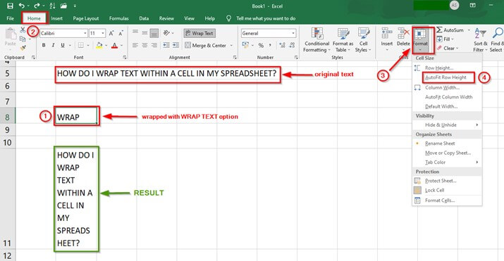
Adjust the row height to make all wrapped text visible
-
Select the cell or range for which you want to adjust the row height.
-
On the Home tab, in the Cells group, click Format.
-
Under Cell Size, do one of the following:
-
To automatically adjust the row height, click AutoFit Row Height.
-
To specify a row height, click Row Height, and then type the row height that you want in the Row height box.
Tip: You can also drag the bottom border of the row to the height that shows all wrapped text.
-
Enter a line break
To start a new line of text at any specific point in a cell:
-
Double-click the cell in which you want to enter a line break.
Tip: You can also select the cell, and then press F2.
-
In the cell, click the location where you want to break the line, and press Alt + Enter.
Need more help?
You can always ask an expert in the Excel Tech Community or get support in the Answers community.
Need more help?
Want more options?
Explore subscription benefits, browse training courses, learn how to secure your device, and more.
Communities help you ask and answer questions, give feedback, and hear from experts with rich knowledge.
When you enter a text string in Excel which exceeds the width of the cell, you can see the text overflowing to the adjacent cell(s).
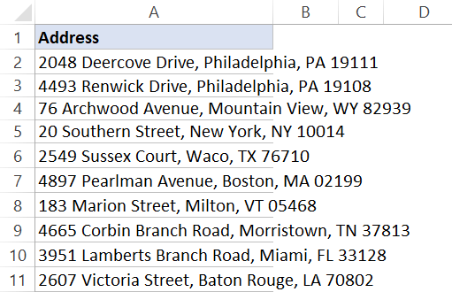
Below is an example where I have some address in column A and these address overflow to the adjacent cells as well.
And in case you have some text in the adjacent cell, the otherwise overflowing text would disappear and you will only see the text that can fit the cell column width.
In both cases, it doesn’t look good and you may want to wrap the text so that the text remains within a cell and not spill over to others.
This can be done using the wrap text feature in Excel.
In this tutorial, I will show you various ways of wrapping text in Excel (including doing it automatically with a single click, using a formula and doing it manually)
So let’s get started!
Wrap text with a Click
Since this is something you may need to do quite often, there is easy access to quickly wrap the text with a click on a button.
Suppose you have the dataset as shown below where you want to wrap text in column A.
Below are the steps to do this:
- Select the entire dataset (column A in this example)
- Click the Home Tab

- In the Alignment group, click on the ‘Wrap text’ button.


That’s It!
All it takes it two-click to quickly wrap the text.
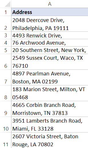
You will get the final result as shown below.
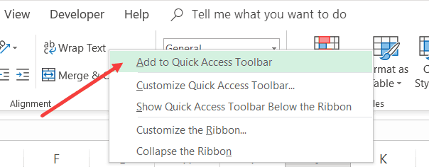
You can further bring down the effort from two to one-click by adding the Wrap text option to the Quick Access Toolbar. To do this. right-click on the Wrap text option and click on ‘Add to Quick Access Toolbar’
This adds an icon to the QAT and when you want to wrap text in any cell, just select it and click this icon in the QAT.
Wrap text with a Keyboard Shortcut
If you’re like me, leaving the keyboard and using a mouse to click even a single button could feel like a waste of time.
Good news is that you can use the below keyboard shortcut to quickly wrap text in all the selected cells.
ALT + H + W (ALY key followed by the H and W keys)
Wrap text with the Format Dialog box
This is my least preferred method, but there is a reason I am including this one in this tutorial (as it can be useful in one specific scenario).
Below are the steps to wrap the text using the Format dialog box:
- Select the cells for which you want to apply the wrap text formatting
- Click the Home tab
- In the Alignment group, click on the Alignment Setting dialog box launcher (it’s a small ’tilted arrow in a box’ icon at the bottom right of the group).

- In the ‘Format Cells’ dialog box that opens, select ‘Alignment’ tab (if not selected already)
- Select the Wrap text option

- Click OK.


The above steps would wrap the text in the selected cells.
Now if you’re thinking why to use this twisted long method when you can use a keyboard shortcut or a single click on the ‘Wrap Text’ button in the ribbon.
In most cases, you should not be using this method, but it can be useful when you want to change a couple of formatting settings. Since the Format Dialog box gives you access to all the formatting options, this may end up saving you some time.
NOTE: You can also use the keyboard shortcut Control + 1 to open the ‘Format Cells’ dialog box.
How Does Excel Decide How Much text to Wrap
When you use the above method, Excel uses the column width to decide how many lines you get after wrapping.
Doing this makes sure that anything that you have in the cell is confined within the cell itself and doesn’t overflow.
In case you change the column width, the text will also adjust to ensure it fits the column width automatically.
Inserting Line Break (Manually, Using Formula, or Find and Replace)
When you apply ‘Wrap Text’ to any cell, Excel determines the line breaks based on the width of the column.
So if there is text which can fit in the existing column width, it will not be wrapped, but in case it can not, Excel will insert the line breaks by first fitting the content in the first line and then moving the rest to the second line (and so on).
By entering a line break manually, you force Excel to move the text to the next line (in the same cell) right after the line break is inserted.
To enter the line break manually, follow the below steps:
- Double-click on the cell in which you want to insert the line break (or press F2). This will get you into the edit mode in the cell
- Place the cursor where you want the line break.
- Use the keyboard shortcut – ALT + ENTER (hold the ALT key and then press Enter).
Note: For this to work, you need to have Wrap Text enabled on the cell. If Wrap Text is not enabled, you will see all the text in one single line, even if you have inserted the line break.
You can also use a CHAR formula to insert a line break (as well as a cool Find and Replace trick to replace any character with a line break).
Both of these methods are covered in this short tutorial on inserting line breaks in Excel.
And in case you want to remove line breaks from cells in Excel, here is a detailed tutorial about it.
Handling Wrapping Too Much Text
Sometimes you may have a lot of text in a cell and when you wrap the text, it may end up making your row height large.
Something as shown below (the text is taken for bookbrowse.com):
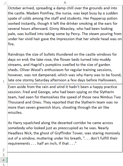
In such a case, you may want to adjust the row height and make it consistent. The downside of this is that not all the text in the cell will be visible, but it makes your worksheet a lot more usable.
Below are the steps to set the row height of the cells:
- Select the cells for which you want to change the row height
- Click the ‘Home’ tab
- In the Cells group, click on the ‘Format’ option

- Click on Row Height

- In the ‘Row Height’ dialog box, enter the value. I am using the value 40 in this example.

- Click OK


The above steps would change the row height and make it all consistent. In case any of the selected cells have text which can not be fit in a cell with the specified height, it will be cut from the bottom.
Don’t worry, the text would still be in the cell. It just won’t be visible.
Excel Text Wrap Not Working – Possible Solutions
In case you find that the Wrap text option is not working as expected and you still see the text as a single line in the cell (or with some missing text), there could be a few possible reasons:
Wrap Text is not enabled
Since it works as a toggle, quickly check whether it’s enabled or not.
If it’s enabled, you will see that this option is highlighted in the Home tab
Cell height needs to be adjusted
When Wrap Text is applied, it moves the extra lines below the first line in the cell. In case your cell row height is less, you may not see the entire wrapped text.
In that case, you need to adjust the cell height.
You change the row height manually by dragging the bottom edge of the row.
Alternatively, you can use the ‘AutoFit Row Height’. This option is available in the ‘Home’ tab in ‘Format’ options.
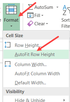
To use the AutoFit option, select all the cells that you want to auto-fit and click on the AutoFit Row Height option.
The Column Width is Already Wide enough
And sometimes there is nothing wrong.
When your column width is wide enough, there is no reason for Excel to wrap the text as it already fits the cell in a single line.
In case you still want the text to split into multiple lines (despite having enough column width), you need to insert the line break manually.
Hope you found this tutorial useful.
You may also like the following Excel tutorials:
- How to Find Merged Cells in Excel
- How to Merge Cells in Excel
- Excel Text to Columns
- Insert Bullet Points in Excel
- How to Insert a Check Mark (Tick Mark) Symbol in Excel
What is Wrap Text in Excel?
The wrap text feature in excel allows displaying lengthy text strings of a cell in multiple lines. This enhances the readability of the worksheet and ensures that the entire cell data is visible at all times. After wrapping text, the row height increases automatically though the column width stays the same. If one changes the column width, the cell content adjusts itself to fit the new width.
For example, in the following image, wrap text has been applied to the string in cell B2. At the same time, column B has been widened.
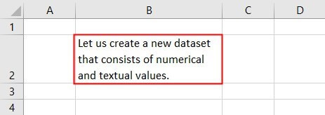
The purpose of wrapping text is to prevent the cell data from spilling to the cells on the right. Moreover, it ensures that a text string is not cut by the border of the adjacent cell. Wrapping text is extremely helpful in worksheets that have a lot of content to display at a time.
Table of contents
- What is Wrap Text in Excel?
- How to Wrap the Text in Excel?
- Method #1–Using the Home tab
- Method #2–Using the “Format Cells” Window
- Method #3–Using the Keyboard Shortcut
- Method #4–Using Line Breaks
- The Reasons “Wrap Text” Feature may not Work in Excel
- Frequently Asked Questions
- Recommended Articles
- How to Wrap the Text in Excel?
How to Wrap the Text in Excel?
Wrap text is a formatting feature of Excel, which changes the appearance of a string without changing the string itself. The methods of wrapping text are listed as follows:
- Method #1–Wrap text using the Home tab
- Method #2–Wrap text using the “format cells” window
- Method #3–Wrap text using the keyboard shortcut
- Method #4–Wrap text using line breaks
Note that methods #1 to #3 wrap text automatically, while method #4 wraps text manually. In method #4, line breaks are inserted at the desired place in a cell. A line break serves as a substitute for the wrap text feature of Excel.
Let us discuss the four methods with the help of examples.
You can download this Wrap Text Excel Template here – Wrap Text Excel Template
Method #1–Using the Home tab
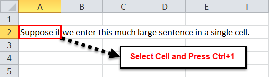
The succeeding image shows a long text string in cell A2. We want to wrap this text in cell A2. Use the “wrap text” option of the Home tab.
The steps to wrap text in excel by using the stated method are listed as follows:
Step 1: Select cell A2 whose text string needs to be wrapped.
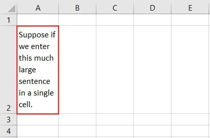
Step 2: From the “alignment” group of the Home tab, click “wrap text.” The text string of cell A2 is displayed in multiple lines, as shown in the succeeding image.
Notice that even after wrapping text, the width of column A stays the same as that of the other columns. However, the height of row 2 increases when this feature is turned on.
Note 1: “Wrap text” is a toggle button that can be turned on and off to wrap and unwrap the text.
Note 2: To wrap the text of multiple cells simultaneously, select all such cells and press the “wrap text” toggle button.
Method #2–Using the “Format Cells” Window
Working on the text string of method #1, we want to wrap the text in cell A2. Use the “format cells” window of Excel.
The steps to wrap text in excel by using “Format Cells” are listed as follows:
- Select cell A2 containing the string to be wrapped. Right-click the selection and choose “format cells” from the context menu.
Alternatively, press the shortcut “Ctrl+1” after selecting the cell.

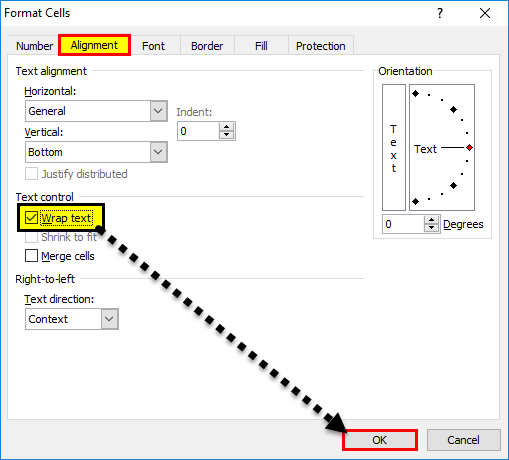
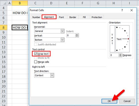
- The “format cells” window opens, as shown in the following image. Click the “alignment” tab. Then, from “text control,” choose the “wrap text” option and click “Ok.”

- The wrap text feature has been applied to cell A2, as shown in the following image. This time also, the width of column A has not changed, but the height of row 2 has increased.

Method #3–Using the Keyboard Shortcut
The succeeding image shows a text string in cell A1. We want to wrap this string of cell A1. Use the keyboard shortcutAn Excel shortcut is a technique of performing a manual task in a quicker way.read more for wrapping text.
The steps to wrap text in excel by using keyboard shortcut are listed as follows:
Step 1: Select cell A1 that consists of the string to be wrapped.
Step 2: Press the shortcut keys “Alt+H+W.” For this shortcut to work, first press the “Alt” key and release it. Next, press and release the “H” key followed by the “W” key.

Step 3: Once the “W” key is released, the “wrap text” feature is applied to the cell selected in step 1. The output is shown in the following image.
Method #4–Using Line Breaks
Working on the text string of method #1, we want to perform the following tasks:
- Apply the wrap text feature in cell A1.
- Insert line breaks manually after the strings “enter,” “large,” and “a” in cell A2.
- Compare the results of applying wrap text with inserting line breaks.
Use the keyboard shortcut for inserting line breaks. Note that both cells A1 and A2 should contain the text string of method #1.
The steps to perform the given tasks are listed as follows:
Step 1: Wrap the text in cell A1 by selecting the cell and choosing “wrap text” from the Home tab. The output is shown in cell A1 of the succeeding image.
Step 2: To insert line breaks, place the cursor in that part of the cell where line breaks are to be inserted. Next, press the keys “Alt+Enter” together.
So, first, place the cursor after the string “enter” and press the given shortcut. The line break is inserted at the end of this string. Likewise, insert line breaks after the strings “large” and “a.”
The result is shown in cell A2 of the following image.
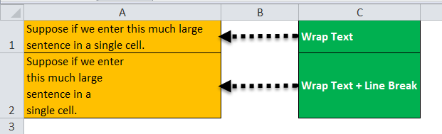
Comparison between applying wrap text and inserting line breaks: It must be noted that when a line break is inserted, the “wrap text” feature is automatically turned on in Excel.
Therefore, when “wrap text” is applied, it is applied alone. However, when a line break is added, it is added in combination with “wrap text.”
The line breaks entered in cell A2 will stay in place even if column A is made wider. Moreover, if “wrap text” is turned off but the line breaks are retained, the string of cell A2 appears in a single line. However, the line breaks inserted in step 2 are visible in the formula bar.
In contrast, when the “wrap text” of cell A1 is disabled, the string appears as a single line, in this cell and the formula bar. So, with wrap text in excel, the cell content can regain its initial appearance with a single click of the toggle button.
The Reasons “Wrap Text” Feature may not Work in Excel
The reasons due to which the wrap text feature may not work in Excel are listed as follows:
- It does not work on merged cells. So, cells need to be unmerged before the wrap text feature can be applied to them.
- It does not work if the cell is already wide enough to display the entire text string. In this case, one can insert line breaks to display the cell content in multiple lines.
- It may not be visible if the height of the row has been set at a very low value. To avoid this, make sure that the height of the row adjusts automatically with the application of the wrap text feature in excel.
Note: To ensure that wrapped text is visible at all times, follow either of the listed techniques in Excel:
- Set the row height to adjust automatically. For this, click the “format” drop-down from the “cells” group of the Home tab. Next, choose “AutoFit row height” from the “cell size” option.
- Enlarge the height of the row manually. For this, place the cursor on the lower border of the row label. The row labels are displayed on the left side of the worksheet. Once the “resizing” mouse pointer appears, drag the lower border of the row downwards to increase the row height.
Frequently Asked Questions
1. What is the wrap text feature and where is it in Excel?
The wrap text feature in excel helps display the content of a cell in multiple lines. With wrap text, the text is wrapped in such a way that the row height increases, but the column width stays the same. Further, the column width can be increased or decreased by the user. The text string adjusts itself automatically with a change in the column width.
However, even after applying the wrap text feature, one can maintain a consistent column width throughout the worksheet. The “wrap text” is a toggle button of Excel, which is available in the “alignment” group of the Home tab.
Note: For more details on the working of the wrap text feature, refer to the examples of this article.
2. List the reasons and state the shortcut of using the wrap text feature in Excel.
The wrap text feature is used in Excel for the following reasons:
• To prevent text strings from being truncated by the adjacent cell
• To avoid overlapping of text strings
• To ensure that the entire cell content is visible
• To improve the readability of large datasets
• To make the worksheet neat, organized, and fit for printing
In Excel, the shortcut of wrapping text is “Alt+H+W.” All the keys must be pressed one after the other in the given sequence. Prior to using this shortcut, ensure that the cell, whose text is to be wrapped, is selected.
3. How to wrap text without expanding the size of the cell in Excel?
After applying the wrap text feature, one can keep either the row height or the column width constant but not both simultaneously. If both (row height and column width) are held constant, the wrapped text will not be visible.
The steps to keep the row height constant are listed as follows:
• Select the cell in which the text is to be wrapped.
• Click the “format” drop-down from the “cells” group of the Home tab.
• From “cell size,” select “row height.”
• In the “row height” window, do not enter any value. Simply click “Ok.”
Now, when the wrap text feature is applied to the selected cell, the row height will remain the same as that of the other rows. On the other hand, the column width already stays constant even after applying the wrap text feature.
However, when the text of a cell is wrapped, it is recommended that one should not prevent a cell from expanding. This is because the basic purpose of wrap text will not be served if the cell is not permitted to enlarge.
Recommended Articles
This has been a guide to wrap text in Excel. Here we discuss how to wrap text in Excel by using the top 4 methods along with shortcuts and examples. You may also look at these useful functions in Excel–
- Format Text in ExcelText formatting in Excel include changing the colour, font name, font size, alignment, font appearance in bold, underlining, italic, background colour of the font cell, and so on.read more
- Separating Text in ExcelThe methods used to separate text in Excel are as follows: 1) Text to Column (Delimited and Fixed Width) 2) Using Excel Formulasread more
- Add Text in Excel FormulaText in Excel Formula allows us to add text values to using the CONCATENATE function or the ampersand (&) symbol.read more
- Change Case in ExcelPROPER, UPPER, and LOWER are the three Excel functions that help in converting the text to proper case, upper case and lower case respectively.read more
Содержание
- Fix data that is cut off in cells
- Wrap text in a cell
- Start a new line in the cell
- Reduce the font size to fit data in the cell
- Reposition the contents of the cell by changing alignment or rotating text
- Change the font size
- Wrap text in a cell
- Wrap text automatically
- Adjust the row height to make all wrapped text visible
- Enter a line break
- Need more help?
- How to Wrap Text in Excel (with shortcut, One Click, and a Formula)
- Wrap text with a Click
- Wrap text with a Keyboard Shortcut
- Wrap text with the Format Dialog box
- How Does Excel Decide How Much text to Wrap
- Inserting Line Break (Manually, Using Formula, or Find and Replace)
- Handling Wrapping Too Much Text
- Excel Text Wrap Not Working – Possible Solutions
- Wrap Text is not enabled
- Cell height needs to be adjusted
- The Column Width is Already Wide enough
Fix data that is cut off in cells
Wrap text, change the alignment, decrease the font size, or rotate your text so that everything you want fits inside a cell.
Wrap text in a cell
You can format a cell so that text wraps automatically.
Select the cells.
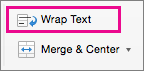
On the Home tab, click Wrap Text.
The text in the selected cell wraps to fit the column width. When you change the column width, text wrapping adjusts automatically.
Note: If all wrapped text is not visible, it might be because the row is set to a specific height. To enable the row to adjust automatically and show all wrapped text, on the Format menu, point to Row, and then click AutoFit.
Start a new line in the cell
Inserting a line break may make text in a cell easier to read.
Double-click in the cell.
Click where you want to insert a line break, and then press CONTROL + OPTION + RETURN .
Reduce the font size to fit data in the cell
Excel can reduce the font size to show all data in a cell. If you enter more content into the cell, Excel will continue to reduce the font size.
Select the cells.
Right-click and select Format Cells.
In the Format Cells dialog box, select the checkbox next to Shrink to fit.
Data in the cell reduces to fit the column width. When you change the column width or enter more data, the font size adjusts automatically.
Reposition the contents of the cell by changing alignment or rotating text
For the optimal display of the data on your sheet, you may want to reposition the text in a cell. You can change the alignment of the cell contents, use indentation for better spacing, or display the data at a different angle by rotating it.
Select the cell or range of cells that contains the data that you want to reposition.
On the Format menu, click Cells.
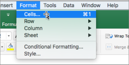
In the Format Cells box, and in the Alignment tab, do any of the following:
Change the horizontal alignment of the cell contents
On the Horizontal pop-up menu, click the alignment that you want.
If you select the Fill option or Center Across Selection option, text rotation will not be available for those cells.
Change the vertical alignment of the cell contents
On the Vertical pop-up menu, click the alignment that you want.
Indent the cell contents
On the Horizontal pop-up menu, click Left (Indent), Right, or Distributed, and then type the amount of indentation (in characters) that you want in the Indent box.
Display the cell contents vertically from top to bottom
Under Orientation, click the box that contains the vertical text.
Rotate the text in a cell
Under Orientation, click or drag the indicator to the angle that you want, or type an angle in the Degrees box.
Restore the default alignment of selected cells
On the Horizontal pop-up menu, click General.
Note: If you save the workbook in another file format, text that was rotated may not display at the correct angle. Most file formats do not support rotation within the full 180 degrees (+90 through –90 degrees) that is possible in the latest versions of Excel. For example, earlier versions of Excel can rotate text only at angles of +90, 0 (zero), or –90 degrees.
Change the font size
Select the cells.
On the Home tab, in the Font size box, enter a different number, or click to reduce the font size.
Источник
Wrap text in a cell
Microsoft Excel can wrap text so it appears on multiple lines in a cell. You can format the cell so the text wraps automatically, or enter a manual line break.
Wrap text automatically
In a worksheet, select the cells that you want to format.
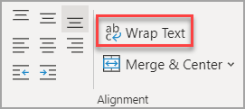
On the Home tab, in the Alignment group, click Wrap Text. (On Excel for desktop, you can also select the cell, and then press Alt + H + W.)
Data in the cell wraps to fit the column width, so if you change the column width, data wrapping adjusts automatically.
If all wrapped text is not visible, it may be because the row is set to a specific height or that the text is in a range of cells that has been merged.
Adjust the row height to make all wrapped text visible
Select the cell or range for which you want to adjust the row height.
On the Home tab, in the Cells group, click Format.
Under Cell Size, do one of the following:
To automatically adjust the row height, click AutoFit Row Height.
To specify a row height, click Row Height, and then type the row height that you want in the Row height box.
Tip: You can also drag the bottom border of the row to the height that shows all wrapped text.
Enter a line break
To start a new line of text at any specific point in a cell:
Double-click the cell in which you want to enter a line break.
Tip: You can also select the cell, and then press F2.
In the cell, click the location where you want to break the line, and press Alt + Enter.
Need more help?
You can always ask an expert in the Excel Tech Community or get support in the Answers community.
Источник
How to Wrap Text in Excel (with shortcut, One Click, and a Formula)
When you enter a text string in Excel which exceeds the width of the cell, you can see the text overflowing to the adjacent cell(s).
Below is an example where I have some address in column A and these address overflow to the adjacent cells as well.
And in case you have some text in the adjacent cell, the otherwise overflowing text would disappear and you will only see the text that can fit the cell column width.
In both cases, it doesn’t look good and you may want to wrap the text so that the text remains within a cell and not spill over to others.
This can be done using the wrap text feature in Excel.
In this tutorial, I will show you various ways of wrapping text in Excel (including doing it automatically with a single click, using a formula and doing it manually)
So let’s get started!
This Tutorial Covers:
Wrap text with a Click
Since this is something you may need to do quite often, there is easy access to quickly wrap the text with a click on a button.
Suppose you have the dataset as shown below where you want to wrap text in column A.
Below are the steps to do this:
- Select the entire dataset (column A in this example)
- Click the Home Tab
- In the Alignment group, click on the ‘Wrap text’ button.
All it takes it two-click to quickly wrap the text.
You will get the final result as shown below.
You can further bring down the effort from two to one-click by adding the Wrap text option to the Quick Access Toolbar. To do this. right-click on the Wrap text option and click on ‘Add to Quick Access Toolbar’
This adds an icon to the QAT and when you want to wrap text in any cell, just select it and click this icon in the QAT.
Wrap text with a Keyboard Shortcut
If you’re like me, leaving the keyboard and using a mouse to click even a single button could feel like a waste of time.
Good news is that you can use the below keyboard shortcut to quickly wrap text in all the selected cells.
Wrap text with the Format Dialog box
This is my least preferred method, but there is a reason I am including this one in this tutorial (as it can be useful in one specific scenario).
Below are the steps to wrap the text using the Format dialog box:
- Select the cells for which you want to apply the wrap text formatting
- Click the Home tab
- In the Alignment group, click on the Alignment Setting dialog box launcher (it’s a small ’tilted arrow in a box’ icon at the bottom right of the group).
- In the ‘Format Cells’ dialog box that opens, select ‘Alignment’ tab (if not selected already)
- Select the Wrap text option
- Click OK.
The above steps would wrap the text in the selected cells.
Now if you’re thinking why to use this twisted long method when you can use a keyboard shortcut or a single click on the ‘Wrap Text’ button in the ribbon.
In most cases, you should not be using this method, but it can be useful when you want to change a couple of formatting settings. Since the Format Dialog box gives you access to all the formatting options, this may end up saving you some time.
NOTE: You can also use the keyboard shortcut Control + 1 to open the ‘Format Cells’ dialog box.
How Does Excel Decide How Much text to Wrap
When you use the above method, Excel uses the column width to decide how many lines you get after wrapping.
Doing this makes sure that anything that you have in the cell is confined within the cell itself and doesn’t overflow.
In case you change the column width, the text will also adjust to ensure it fits the column width automatically.
Inserting Line Break (Manually, Using Formula, or Find and Replace)
When you apply ‘Wrap Text’ to any cell, Excel determines the line breaks based on the width of the column.
So if there is text which can fit in the existing column width, it will not be wrapped, but in case it can not, Excel will insert the line breaks by first fitting the content in the first line and then moving the rest to the second line (and so on).
By entering a line break manually, you force Excel to move the text to the next line (in the same cell) right after the line break is inserted.
To enter the line break manually, follow the below steps:
- Double-click on the cell in which you want to insert the line break (or press F2). This will get you into the edit mode in the cell
- Place the cursor where you want the line break.
- Use the keyboard shortcut – ALT + ENTER (hold the ALT key and then press Enter).
Note: For this to work, you need to have Wrap Text enabled on the cell. If Wrap Text is not enabled, you will see all the text in one single line, even if you have inserted the line break.
You can also use a CHAR formula to insert a line break (as well as a cool Find and Replace trick to replace any character with a line break).
Both of these methods are covered in this short tutorial on inserting line breaks in Excel.
And in case you want to remove line breaks from cells in Excel, here is a detailed tutorial about it.
Handling Wrapping Too Much Text
Sometimes you may have a lot of text in a cell and when you wrap the text, it may end up making your row height large.
Something as shown below (the text is taken for bookbrowse.com):
In such a case, you may want to adjust the row height and make it consistent. The downside of this is that not all the text in the cell will be visible, but it makes your worksheet a lot more usable.
Below are the steps to set the row height of the cells:
- Select the cells for which you want to change the row height
- Click the ‘Home’ tab
- In the Cells group, click on the ‘Format’ option
- Click on Row Height
- In the ‘Row Height’ dialog box, enter the value. I am using the value 40 in this example.
- Click OK
The above steps would change the row height and make it all consistent. In case any of the selected cells have text which can not be fit in a cell with the specified height, it will be cut from the bottom.
Don’t worry, the text would still be in the cell. It just won’t be visible.
Excel Text Wrap Not Working – Possible Solutions
In case you find that the Wrap text option is not working as expected and you still see the text as a single line in the cell (or with some missing text), there could be a few possible reasons:
Wrap Text is not enabled
Since it works as a toggle, quickly check whether it’s enabled or not.
If it’s enabled, you will see that this option is highlighted in the Home tab
Cell height needs to be adjusted
When Wrap Text is applied, it moves the extra lines below the first line in the cell. In case your cell row height is less, you may not see the entire wrapped text.
In that case, you need to adjust the cell height.
You change the row height manually by dragging the bottom edge of the row.
Alternatively, you can use the ‘AutoFit Row Height’. This option is available in the ‘Home’ tab in ‘Format’ options.
To use the AutoFit option, select all the cells that you want to auto-fit and click on the AutoFit Row Height option.
The Column Width is Already Wide enough
And sometimes there is nothing wrong.
When your column width is wide enough, there is no reason for Excel to wrap the text as it already fits the cell in a single line.
In case you still want the text to split into multiple lines (despite having enough column width), you need to insert the line break manually.
Hope you found this tutorial useful.
You may also like the following Excel tutorials:
Источник
What is Wrap Text in Excel?
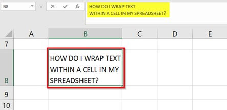
Wrap Text is a feature in Microsoft Excel spreadsheets that wraps or fits the contents of a cell within the boundaries of the cell. It auto-sizes the row height and column width of the selected cell.
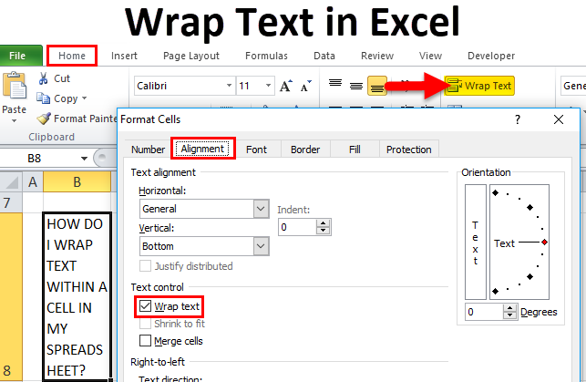
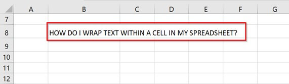
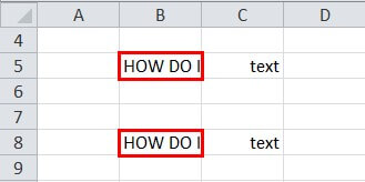
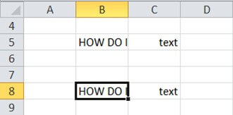
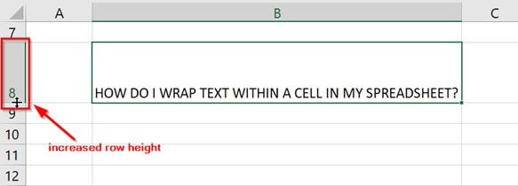
For example, the text in cell B8 – HOW DO I WRAP TEXT WITHIN A CELL IN MY SPREADSHEET? is spread across the columns C, D, E, and F if there is no text or content in adjacent cell C8.
OR
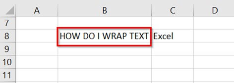
The cell is cut off since there is text “Excel” in adjacent cell C8 as shown below
When we apply the WRAP Text feature, the text or content is contained within the boundaries of the cell as shown in the below image
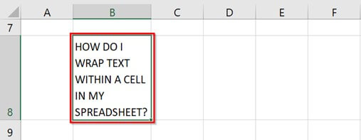
Wrap Text wraps or fits the cell contents on multiple lines, rather than a single or one long line without overlapping the text content to another adjacent cell.
Key Highlights
- We can use Wrap text in Excel to wrap or enclose a long string of content in a single cell.
- Wrap text displays the first 1,024 characters in a cell. If the number of characters exceeds the limit, it is displayed as **
- We can toggle the Wrap Text option ON and OFF in Excel to apply and remove the feature to the selected cell content
- When we modify the column width, Microsoft Excel adjusts the text or content wrapping automatically
- We can also wrap texts in a cell by adjusting row height along with Autofit option in the Excel Ribbon
How to Wrap Text in Excel?
You can download this Wrap Text in Excel Template here – Wrap Text in Excel Template
1] AUTOMATIC WRAP TEXT
METHOD 1: Wrap Text in Excel using Ribbon
Example #1
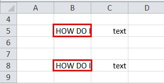
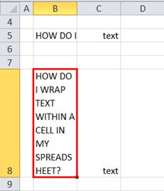
In the below table, there is a long string of text in cells B5 and B8. We want to wrap the text of cell B8 using the Excel Ribbon.
Solution:
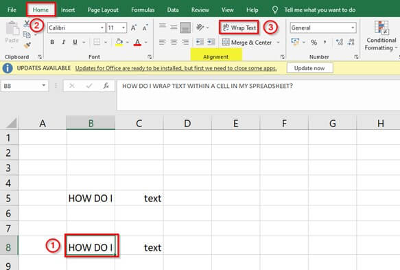
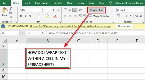
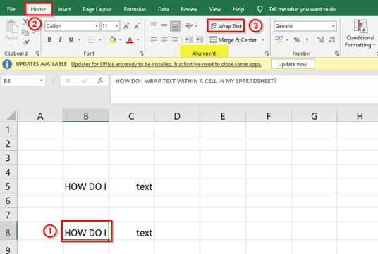
Step 1: Select cell B8
Step 2: Go to the Home tab and click Wrap Text in the Alignment Group as shown in the below image.
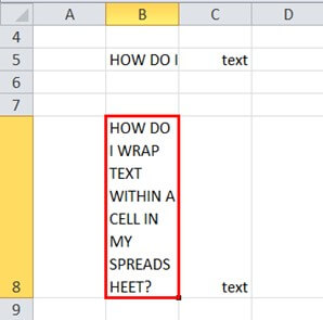
Wrap text feature wraps up the text- HOW DO I WRAP TEXT WITHIN MY SPREADSHEET within single cell B8 as shown below
Note:
- If we initially set the row height to a certain value or manually set a row height, or adjust column width by clicking on the right bottom border of a row header and dragging the separator towards left or right, there will be no change in the row height or column width when we click the Wrap Text option.
- If there is a change, then we must simply double-click the bottom border of a row header to fix this.
METHOD 2: WRAP Text in Excel using the FORMAT CELLS option
Example #2
Consider the same example as above. Here, we want to wrap the text in cell B8 using the Format Cells option
Solution:
Step 1: Select the cell or group of cells that contain the long string of text.
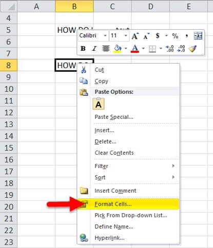
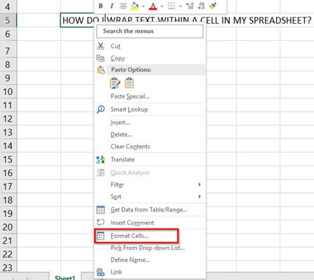
Step 2: Right-click on the selected cell and go to the Format Cells option
OR
Select the dropdown option in the Font Group of the Home tab of the Excel ribbon.
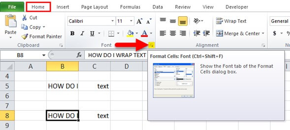
This opens up the Format Cells dialog box as shown below
Note: We can also use Ctrl + 1 to open the Format Cells dialog box.
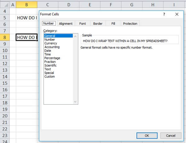
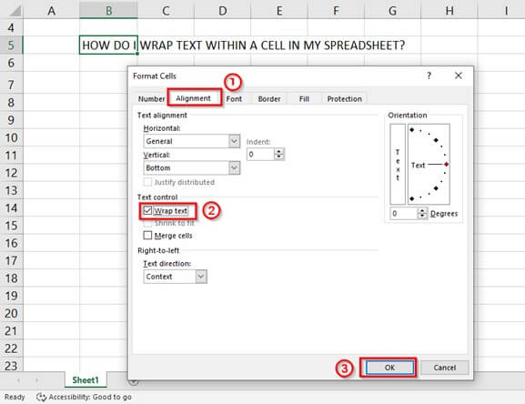
Step 3: In the Format Cells dialog box, select Alignment>Wrap Text checkbox and click OK.
This wraps up or fits the B8 cell content within the limits of the cell as shown below
2] MANUAL WRAP TEXT
METHOD 3: Wrap Text in Excel by Adjusting Rows and Columns
Example #3
In this example, we want to wrap the text by Adjusting Row height and Column Width
Solution:
Step 1: Place the cross (+) at the edge of the desired column as shown in the below image
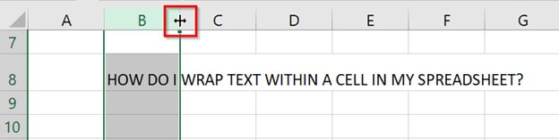
Step 2: Hold and move the cross towards the right and stop until the text fills in the cell B8
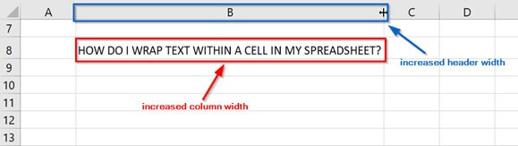
This will wrap the text in a single cell B8 but with increased column width as shown in the below image
If we increase the row height only the row header size will increase, it will not wrap the text,
To solve this problem,
Step 3: Click on the Wrap Text option in the Excel ribbon and the text in cell B8 is wrapped as shown in the below image
METHOD 4: Wrap Text in Excel by Adding Line Breaks
Example #4
Here, we want to Wrap the text in cell B8 by Adding Line Breaks
Solution:
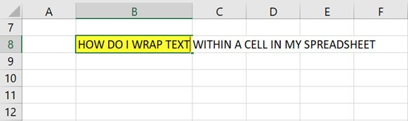
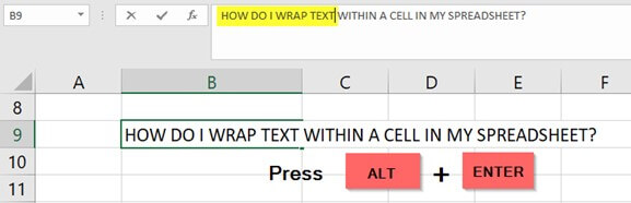
Step 1: Place the cursor at the position(highlighted in yellow) where the data exceeds the boundaries of cell B8
Now,
Step 2: Press Alt + Enter to add a line break
It will break the line into two to fit(wrap) the text into a single cell B8
Advantages of Wrap Text
- With the Wrap text functionality of Microsoft Excel, we can view all the data or information within a single cell.
- It makes reading easier and fits the content better in a cell suitable for printing the worksheet.
- If we wrap the text of the entire Excel worksheet, the column width becomes consistent throughout and gives a better viewing experience.
Things to Remember
- If we want to unwrap the text, we need to follow the same steps that we use for wrapping the text.
- The Wrap Text option in excel is not applicable to merged cells.
- If we fix the row height the wrapping will not be visible sometimes. We can make it visible by choosing the Autofit Row Height option in the Format section of the Home
Frequently Asked Questions (FAQs)
Q1) How do I enable text wrapping in sheets?
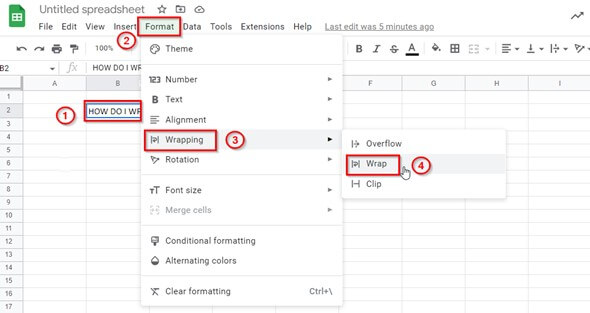
Answer: To wrap text in Google sheets,
- Select the cell of the data you want to wrap
- Click on Format > Wrapping > Wrap
Q2) Where is wrap text in excel?
Answer: To locate Wrap Text,
- Select the cell of the data you want to wrap
- Click on Home > Wrap Text
Q3) Why can’t I wrap text in Excel?
Answer: The possible reason that sometimes the wrapped text is not visible is that we have manually set the row height to a certain value. To solve this problem, we should
- Select the cell of the data we want to wrap
- Click on Home > Format > Autofit Row Height
Q4) How do I set wrap text as default in Excel?
Answer: To set wrap text in Excel as default,
- Select the cell of the data you want to wrap
- Right-click on the cell to get a dropdown menu
- Click on Format Cells > Alignment > Wrap text > OK
Recommended Articles
The article is a guide to Wrap Text in Excel. EDUCBA recommends the below-given articles to get more Excel-related information.
- Compare Text in Excel
- Excel Text with Formula
- VBA Text
- Formatting Text in Excel