
Содержание
- Свойства и методы Worksheet
- Краткое руководство к рабочему листу VBA
- Вступление
- Доступ к рабочему листу
- Использование индекса для доступа к рабочему листу
- Использование кодового имени рабочего листа
- Активный лист
- Объявление объекта листа
- Доступ к рабочему листу в двух словах
- Добавить рабочий лист
- Удалить рабочий лист
- Цикл по рабочим листам
- Использование коллекции листов
- Заключение
Свойства и методы Worksheet

Мечтатель начинает с чистого листа бумаги и переосмысливает мир
Эта статья содержит полное руководство по использованию Excel
VBA Worksheet в Excel VBA. Если вы хотите узнать, как что-то сделать быстро, ознакомьтесь с кратким руководством к рабочему листу VBA ниже.
Если вы новичок в VBA, то эта статья — отличное место для начала. Мне нравится разбивать вещи на простые термины и объяснять их на простом языке.
Вы можете прочитать статью от начала до конца, так как она написана в логическом порядке. Или, если предпочитаете, вы можете использовать оглавление ниже и перейти непосредственно к теме по вашему выбору.
Краткое руководство к рабочему листу VBA
В следующей таблице приведен краткий обзор различных методов
Worksheet .
Примечание. Я использую Worksheet в таблице ниже, не указывая рабочую книгу, т.е. Worksheets, а не ThisWorkbook.Worksheets, wk.Worksheets и т.д. Это сделано для того, чтобы примеры были понятными и удобными для чтения. Вы должны всегда указывать рабочую книгу при использовании Worksheets . В противном случае активная рабочая книга будет использоваться по умолчанию.
| Задача | Исполнение |
| Доступ к рабочему листу по имени |
Worksheets(«Лист1») |
| Доступ к рабочему листу по позиции слева |
Worksheets(2) Worksheets(4) |
| Получите доступ к самому левому рабочему листу |
Worksheets(1) |
| Получите доступ к самому правому листу |
Worksheets(Worksheets.Count) |
| Доступ с использованием кодового имени листа (только текущая книга) |
Смотри раздел статьи Использование кодового имени |
| Доступ по кодовому имени рабочего листа (другая рабочая книга) |
Смотри раздел статьи Использование кодового имени |
| Доступ к активному листу | ActiveSheet |
| Объявить переменную листа | Dim sh As Worksheet |
| Назначить переменную листа | Set sh = Worksheets(«Лист1») |
| Добавить лист | Worksheets.Add |
| Добавить рабочий лист и назначить переменную |
Worksheets.Add Before:= Worksheets(1) |
| Добавить лист в первую позицию (слева) |
Set sh =Worksheets.Add |
| Добавить лист в последнюю позицию (справа) |
Worksheets.Add after:=Worksheets(Worksheets.Count) |
| Добавить несколько листов | Worksheets.Add Count:=3 |
| Активировать рабочий лист | sh.Activate |
| Копировать лист | sh.Copy |
| Копировать после листа | sh1.Copy After:=Sh2 |
| Скопировать перед листом | sh1.Copy Before:=Sh2 |
| Удалить рабочий лист | sh.Delete |
| Удалить рабочий лист без предупреждения |
Application.DisplayAlerts = False sh.Delete Application.DisplayAlerts = True |
| Изменить имя листа | sh.Name = «Data» |
| Показать/скрыть лист | sh.Visible = xlSheetHidden sh.Visible = xlSheetVisible sh.Name = «Data» |
| Перебрать все листы (For) | Dim i As Long For i = 1 To Worksheets.Count Debug.Print Worksheets(i).Name Next i |
| Перебрать все листы (For Each) | Dim sh As Worksheet For Each sh In Worksheets Debug.Print sh.Name Next |
Вступление
Три наиболее важных элемента VBA — это Рабочая книга, Рабочий лист и Ячейки. Из всего кода, который вы пишете, 90% будут включать один или все из них.
Наиболее распространенное использование Worksheet в VBA для доступа к его ячейкам. Вы можете использовать его для защиты, скрытия, добавления, перемещения или копирования листа.
Тем не менее, вы будете в основном использовать его для выполнения некоторых действий с одной или несколькими ячейками на листе.
Использование Worksheets более простое, чем использование рабочих книг. С книгами вам может потребоваться открыть их, найти, в какой папке они находятся, проверить, используются ли они, и так далее. С рабочим листом он либо существует в рабочей книге, либо его нет.
Доступ к рабочему листу
В VBA каждая рабочая книга имеет коллекцию рабочих листов. В этой коллекции есть запись для каждого рабочего листа. Эта коллекция называется просто Worksheets и используется очень похоже на коллекцию Workbooks. Чтобы получить доступ к рабочему листу, достаточно указать имя.
Приведенный ниже код записывает «Привет Мир» в ячейках A1 на листах: Лист1, Лист2 и Лист3 текущей рабочей книги.
Коллекция Worksheets всегда принадлежит книге. Если мы не указываем рабочую книгу, то активная рабочая книга используется по умолчанию.
Скрыть рабочий лист
В следующих примерах показано, как скрыть и показать лист.
Если вы хотите запретить пользователю доступ к рабочему листу, вы можете сделать его «очень скрытым». Это означает, что это может быть сделано видимым только кодом.
Защитить рабочий лист
Другой пример использования Worksheet — когда вы хотите защитить его.
Индекс вне диапазона
При использовании Worksheets вы можете получить сообщение об ошибке:
Run-time Error 9 Subscript out of Range

Это означает, что вы пытались получить доступ к рабочему листу, который не существует. Это может произойти по следующим причинам:
- Имя Worksheet , присвоенное рабочим листам, написано неправильно.
- Название листа изменилось.
- Рабочий лист был удален.
- Индекс был большим, например Вы использовали рабочие листы (5), но есть только четыре рабочих листа
- Используется неправильная рабочая книга, например Workbooks(«book1.xlsx»).Worksheets(«Лист1») вместо
Workbooks(«book3.xlsx»).Worksheets («Лист1»).
Если у вас остались проблемы, используйте один из циклов из раздела «Циклы по рабочим листам», чтобы напечатать имена всех рабочих листов коллекции.
Использование индекса для доступа к рабочему листу
До сих пор мы использовали имя листа для доступа к листу. Указатель относится к положению вкладки листа в рабочей книге. Поскольку положение может быть легко изменено пользователем, не рекомендуется использовать это.
В следующем коде показаны примеры использования индекса.
В приведенном выше примере я использовал Debug.Print для печати в Immediate Window. Для просмотра этого окна выберите «Вид» -> «Immediate Window » (Ctrl + G).


Использование кодового имени рабочего листа
Лучший способ получить доступ к рабочему листу — использовать кодовое имя. Каждый лист имеет имя листа и кодовое имя. Имя листа — это имя, которое отображается на вкладке листа в Excel.
Изменение имени листа не приводит к изменению кодового имени, что означает, что ссылка на лист по кодовому имени — отличная идея.
Если вы посмотрите в окне свойств VBE, вы увидите оба имени. На рисунке вы можете видеть, что кодовое имя — это имя вне скобок, а имя листа — в скобках.

Вы можете изменить как имя листа, так и кодовое имя в окне свойств листа (см. Изображение ниже).

Если ваш код ссылается на кодовое имя, то пользователь может изменить имя листа, и это не повлияет на ваш код. В приведенном ниже примере мы ссылаемся на рабочий лист напрямую, используя кодовое имя.
Это делает код легким для чтения и безопасным от изменения пользователем имени листа.
Кодовое имя в других книгах
Есть один недостаток использования кодового имени. Он относится только к рабочим листам в рабочей книге, которая содержит код, т.е. ThisWorkbook.
Однако мы можем использовать простую функцию, чтобы найти кодовое имя листа в другой книге.
Использование приведенного выше кода означает, что если пользователь изменит имя рабочего листа, то на ваш код это не повлияет.
Существует другой способ получения имени листа внешней рабочей книги с использованием кодового имени. Вы можете использовать элемент VBProject этой Рабочей книги.
Вы можете увидеть, как это сделать, в примере ниже. Я включил это, как дополнительную информацию, я бы рекомендовал использовать метод из предыдущего примера, а не этот.
Резюме кодового имени
Ниже приведено краткое описание использования кодового имени:
- Кодовое имя рабочего листа может быть использовано непосредственно в коде, например. Sheet1.Range
- Кодовое имя будет по-прежнему работать, если имя рабочего листа будет изменено.
- Кодовое имя может использоваться только для листов в той же книге, что и код.
- Везде, где вы видите ThisWorkbook.Worksheets («имя листа»), вы можете заменить его кодовым именем рабочего листа.
- Вы можете использовать функцию SheetFromCodeName сверху, чтобы получить кодовое имя рабочих листов в других рабочих книгах.
Активный лист
Объект ActiveSheet ссылается на рабочий лист, который в данный момент активен. Вы должны использовать ActiveSheet только в том случае, если у вас есть особая необходимость ссылаться на активный лист.
В противном случае вы должны указать рабочий лист, который вы используете.
Если вы используете метод листа, такой как Range, и не упоминаете лист, он по умолчанию будет использовать активный лист.
Объявление объекта листа
Объявление объекта листа полезно для того, чтобы сделать ваш код более понятным и легким для чтения.
В следующем примере показан код для обновления диапазонов ячеек. Первый Sub не объявляет объект листа. Вторая подпрограмма объявляет объект листа, и поэтому код намного понятнее.
Вы также можете использовать ключевое слово With с объектом листа, как показано в следующем примере.
Доступ к рабочему листу в двух словах
Из-за множества различных способов доступа к рабочему листу вы можете быть сбитыми с толку. Так что в этом разделе я собираюсь разбить его на простые термины.
- Если вы хотите использовать тот лист, который активен в данный момент, используйте ActiveSheet.
2. Если лист находится в той же книге, что и код, используйте кодовое имя.
3. Если рабочая таблица находится в другой рабочей книге, сначала получите рабочую книгу, а затем получите рабочую таблицу.
Если вы хотите защитить пользователя от изменения имени листа, используйте функцию SheetFromCodeName из раздела «Имя кода».
Добавить рабочий лист
Примеры в этом разделе показывают, как добавить новую рабочую таблицу в рабочую книгу. Если вы не предоставите никаких аргументов для функции Add, то новый рабочий лист будет помещен перед активным рабочим листом.
Когда вы добавляете рабочий лист, он создается с именем по умолчанию, например «Лист4». Если вы хотите изменить имя, вы можете легко сделать это, используя свойство Name.
В следующем примере добавляется новый рабочий лист и изменяется имя на «Счета». Если лист с именем «Счета» уже существует, вы получите сообщение об ошибке.
В предыдущем примере вы добавляете листы по отношению к активному листу. Вы также можете указать точную позицию для размещения листа.
Для этого вам нужно указать, какой лист новый лист должен быть вставлен до или после. Следующий код показывает вам, как это сделать.
Удалить рабочий лист
Чтобы удалить лист, просто вызовите Delete.
Excel отобразит предупреждающее сообщение при удалении листа. Если вы хотите скрыть это сообщение, вы можете использовать код ниже:
Есть два аспекта, которые нужно учитывать при удалении таблиц.
Если вы попытаетесь получить доступ к рабочему листу после его удаления, вы получите ошибку «Subscript out of Range», которую мы видели в разделе «Доступ к рабочему листу».
Вторая проблема — когда вы назначаете переменную листа. Если вы попытаетесь использовать эту переменную после удаления листа, вы получите ошибку автоматизации, подобную этой:
Run-Time error -21147221080 (800401a8′) Automation Error
Если вы используете кодовое имя рабочего листа, а не переменную, это приведет к сбою Excel, а не к ошибке автоматизации.
В следующем примере показано, как происходят ошибки автоматизации.
Если вы назначите переменную Worksheet действительному рабочему листу, он будет работать нормально.
Цикл по рабочим листам
Элемент «Worksheets» — это набор рабочих листов, принадлежащих рабочей книге. Вы можете просмотреть каждый лист в коллекции рабочих листов, используя циклы «For Each» или «For».
В следующем примере используется цикл For Each.
В следующем примере используется стандартный цикл For.
Вы видели, как получить доступ ко всем открытым рабочим книгам и как получить доступ ко всем рабочим листам в ThisWorkbook. Давайте сделаем еще один шаг вперед — узнаем, как получить доступ ко всем рабочим листам во всех открытых рабочих книгах.
Примечание. Если вы используете код, подобный этому, для записи на листы, то сначала сделайте резервную копию всего, так как в итоге вы можете записать неверные данные на все листы.
Использование коллекции листов
Рабочая книга имеет еще одну коллекцию, похожую на Worksheets под названием Sheets. Это иногда путает пользователей. Чтобы понять, в первую очередь, вам нужно знать о типе листа, который является диаграммой.
В Excel есть возможность создать лист, который является диаграммой. Для этого нужно:
- Создать диаграмму на любом листе.
- Щелкнуть правой кнопкой мыши на графике и выбрать «Переместить».
- Выбрать первый вариант «Новый лист» и нажмите «ОК».
Теперь у вас есть рабочая книга, в которой есть типовые листы и лист-диаграмма.
- Коллекция «Worksheets » относится ко всем рабочим листам в рабочей книге. Не включает в себя листы типа диаграммы.
- Коллекция Sheets относится ко всем листам, принадлежащим книге, включая листы типовой диаграммы.
Ниже приведены два примера кода. Первый проходит через все листы в рабочей книге и печатает название листа и тип листа. Второй пример делает то же самое с коллекцией Worksheets.
Чтобы опробовать эти примеры, вы должны сначала добавить лист-диаграмму в свою книгу, чтобы увидеть разницу.
Если у вас нет листов диаграмм, то использование коллекции Sheets — то же самое, что использование коллекции WorkSheets.
Заключение
На этом мы завершаем статью о Worksheet VBA. Я надеюсь, что было полезным.
Три наиболее важных элемента Excel VBA — это рабочие книги, рабочие таблицы, диапазоны и ячейки.
Эти элементы будут использоваться практически во всем, что вы делаете. Понимание их сделает вашу жизнь намного проще и сделает изучение VBA увлекательнее.
Источник
Lesson 13: Working with Worksheets
/en/excel2007/aligning-text/content/
Introduction
 It is important that you know how to effectively manage your worksheets. By default, three worksheets appear in each new workbook. In this lesson, you will learn how to name, add, delete, group, and ungroup worksheets. Additionally, you will learn how to freeze specific parts of the worksheet so they are always visible.
Worksheets
Download the example to work along with the video.
Naming worksheets
When you open an Excel workbook, there are three sheets by default, and the default name on the tabs are Sheet1, Sheet2, and Sheet3. These are not very informative names. Excel 2007 allows you to create a meaningful name for each worksheet in a workbook so you can quickly locate information.
To name a worksheet:
- Right-click the sheet tab to select it.
- Choose Rename from the menu that appears. The text is highlighted by a black box.
- Type a new name for the worksheet.
- Click off of the tab. The worksheet now assumes the descriptive name defined.
OR - Click the Format command in the Cells group on the Home tab.
- Select Rename Sheet. The text is highlighted by a black box.
- Type a new name for the worksheet.
- Click off of the tab. The worksheet now assumes the descriptive name defined.
Inserting worksheets
You can change the default number of sheets that appears by clicking the Microsoft Office button and choosing Excel Options. You also have the ability to insert new worksheets if needed while you are working.
To insert a new worksheet:
- Left-click the Insert Worksheet icon. A new sheet will appear. It will be named Sheet4, Sheet5, or whatever the next sequential sheet number may be in the workbook.
- OR
- Press the Shift and the F11 keys on your keyboard.
Deleting worksheets
Any worksheet can be deleted from a workbook, including those that have data in it. Remember, a workbook must contain at least one worksheet.
To delete one or more worksheets:
- Click on the sheet(s) you want to delete.
- Right-click the sheet(s), and a menu appears.
- Select Delete.
- OR
- Select the sheet you want to remove.
- Click the drop-down arrow next to Delete in the Cells group on the Home tab.
- From the menu that appears, select Delete Sheet.
Grouping and ungrouping worksheets
A workbook is a multi-page Excel document that contains multiple worksheets. Sometimes you will want to work with the worksheets one at a time as if each is a single unit. Other times, the same information or formatting may need to be added to every worksheet.
Worksheets can be combined together into a group. Grouping worksheets allows you to apply identical formulas and/or formatting across all of the worksheets in the group. When you group worksheets, any changes made to one worksheet will be changed in any other worksheets in the group.
To group contiguous worksheets:
- Select the first sheet you want to group.
- Press and hold the Shift key on your keyboard.
- Click the last sheet you want to group.
- Release the Shift key.
- The sheets are now grouped. All of the sheets between the first sheet and last sheet selected are part of the group. The sheet tabs will appear white for the grouped sheets.
- Make any changes to one sheet, and the changes will appear in all the grouped sheets.
To group noncontiguous sheets:
- Select the first sheet you want to group.
- Press and hold the Ctrl key on your keyboard.
- Click the next sheet you want to group.
- Continuing clicking the sheets you want to group.
- Release the Control key.
- The sheets are now grouped. The sheet tabs will appear white for the grouped sheets. Only the sheets selected are part of the group.
- Make any changes to one sheet, and the changes will appear in all the grouped sheets.
To ungroup worksheets:
- Right-click one of the sheets.
- Select Ungroup from the list.
Freezing worksheet panes
The ability to freeze, or lock, specific rows or columns in your spreadsheet is a useful feature in Excel. It is called freezing panes. When you freeze panes, you select rows or columns that will remain visible all the time, even as you are scrolling. This is particularly useful when working with large spreadsheets.
To freeze a row:
- Select the row below the one you want frozen. For example, if you want rows 1 and 2 to appear at the top even as you scroll, select row 3.
- Click the View tab.
- Click the Freeze Pane command in the Window group.
- Choose Freeze Panes. A thin, black line appears below everything that is frozen in place.
- Scroll down in the worksheet to see the pinned rows.
To unfreeze a pane:
- Click the Freeze Pane command.
- Select the Unfreeze command.
To freeze a column:
- Select the column to the right of the column(s) you want frozen. For example, if you want columns A and B to always appear on the left, select column C.
- Click the View tab.
- Click the Freeze Pane command in the Window group.
- Choose Freeze Pane. A thin, black line appears to the right of the frozen area.
- Scroll across in the worksheet to see the pinned columns.
Challenge!
Use the Inventory workbook or any workbook you choose to complete this challenge.
- Rename Sheet1 to January, Sheet2 to February, and Sheet3 to March.
- Insert two worksheets, and name them April and May.
- If necessary, move the April and May worksheets so they are immediately following the March sheet.
- Use the Grouping feature so all of the sheets contain the same information as the January sheet.
- Delete the May sheet.
- Freeze rows 1 and 2 on the January sheet.
/en/excel2007/using-templates/content/
Chapter 4. Managing Worksheets and Workbooks
So far youâve
learned how to create a basic worksheet with a
table of data. Thatâs great for getting started,
but as power users, professional accountants, and
other Excel jockeys quickly learn, some of the
most compelling reasons to use Excel involve
multiple tables that share
information and interact with each other.
For example, say you want to track the
performance of your company: you create one table
summarizing your firmâs yearly sales, another
listing expenses, and a third analyzing
profitability and making predictions for the
coming year. If you create these tables in
different spreadsheet files, then you have to copy
shared information from one location to another,
all without misplacing a number or making a
mistake. And whatâs worse, with data scattered in
multiple places, youâre missing the chance to use
some of Excelâs niftiest charting and analytical
tools. Similarly, if you try cramming a bunch of
tables onto the same worksheet page, then you can
quickly create formatting and cell management
problems.
Fortunately, a better solution exists. Excel
lets you create spreadsheets
with multiple pages of data, each of which can
conveniently exchange information with other
pages. Each page is called a worksheet, and a
collection of one or more worksheets is called a
workbook (which is also
sometimes called a spreadsheet
file). In this chapter, youâll learn
how to manage the worksheets in a workbook. Youâll
also take a look at two more all-purpose Excel
features: Find and Replace (a tool for digging
through worksheets in search of specific data) and
the spell checker.
Worksheets and Workbooks
Many workbooks
contain more than one table of information. For
example, you might have a list of your bank
account balances and a list of items repossessed
from your home in the same financial planning
spreadsheet. You might find it a bit challenging
to arrange these different tables. You could stack
them (Figure 4-1) or place them side by side
(Figure
4-2), but neither solution is
perfect.
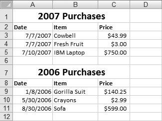
Figure 4-1. Stacking tables on top of each other is
usually a bad idea. If you need to add more data
to the first table, then you have to move the
second table. Youâll also have trouble properly
resizing or formatting columns because each column
contains data from two different tables.
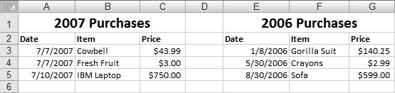
Figure 4-2. Youâre somewhat better off putting tables
side by side, separated by a blank column, than
you are stacking them, but this method can create
problems if you need to add more columns to the
first table. It also makes for a lot of
side-to-side scrolling.
Most Excel masters agree that the best way
to arrange separate tables of information is to
use separate worksheets for each table. When you
create a new workbook, Excel automatically fills
it with three blank worksheets named Sheet1,
Sheet2, and Sheet3. Often, youâll work exclusively
with the first worksheet (Sheet1), and not even
realize that you have two more blank worksheets to
play withânot to mention the ability to add plenty
more.
To move from one worksheet to another, you
have a few choices:
-
Click the worksheet tabs at the bottom of
Excelâs grid window (just above the status bar),
as shown in Figure
4-3. -
Press Ctrl+Page Down to move to the next
worksheet. For example, if youâre currently in
Sheet1, this key sequence jumps you to
Sheet2. -
Press Ctrl+Page Up to move to the previous
worksheet. For example, if youâre currently in
Sheet2, this key sequence takes you back to
Sheet1.
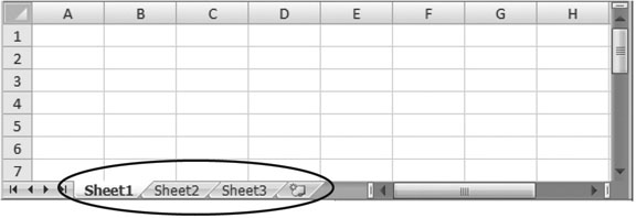
Figure 4-3. Worksheets provide a good way to
organize multiple tables of data. To move from one
worksheet to another, click the appropriate
Worksheet tab at the bottom of the grid. Each
worksheet contains a fresh grid of cellsâfrom A1
all the way to XFD1048576.
Excel keeps track of the active
cell in each worksheet. That means if youâre in
cell B9 in Sheet1, and then move to Sheet2, when
you jump back to Sheet1 youâll automatically
return to cell B9.
Tip
Excel includes some interesting viewing
features that let you look at two different
worksheets at the same time, even if these
worksheets are in the same workbook. Youâll learn
more about custom views in Chapter
7.
Adding, Removing, and Hiding
Worksheets
When
you open a fresh workbook in Excel, you
automatically get three blank worksheets in it.
You can easily add more worksheets. Just click the
Insert Worksheet button, which appears immediately
to the right of your last worksheet tab (Figure
4-4). You can also use the Home â Cells â
Insert â Insert Sheet command, which works the
same way but inserts a new worksheet immediately
to the left of the current
worksheet. (Donât panic; Section
4.1.2 shows how you can rearrange
worksheets after the fact.)
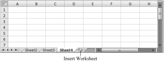
Figure 4-4. Every time you click the Insert Worksheet
button, Excel inserts a new worksheet after your
existing worksheets and assigns it a new name. For
example, if you start with the standard Sheet1,
Sheet2, and Sheet3 and click the Insert Worksheet
button, then Excel adds a new worksheet namedâyou
guessed itâSheet4.
If you continue adding worksheets,
youâll eventually find that all the worksheet tabs
wonât fit at the bottom of your workbook window.
If you run out of space, you need to use the
scroll buttons (which
are immediately to the left of the worksheet tabs)
to scroll through the list of worksheets. Figure
4-5 shows the scroll buttons.
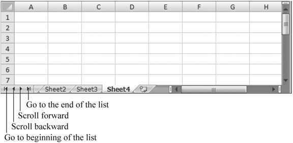
Figure 4-5. Using the scroll buttons, you can
move between worksheets one at a time or jump
straight to the first or last tab. These scroll
buttons control only which tabs you seeâyou still
need to click the appropriate tab to move to the
worksheet you want to work on.
Tip
If you have a huge number of worksheets
and they donât all fit in the strip of worksheet
tabs, thereâs an easier way to jump around.
Right-click the scroll buttons to pop up a list
with all your worksheets.
You can then move to the worksheet you want by
clicking it in the list.
Removing a
worksheet is just as easy as adding one. Simply
move to the worksheet you want to get rid of, and
then choose Home â Cells â Delete â Delete Sheet
(you can also right-click a worksheet tab and
choose Delete). Excel wonât complain if you ask it
to remove a blank worksheet, but if you try to
remove a sheet that contains any data, it presents
a warning message asking for your confirmation.
Also, if youâre down to one last worksheet, Excel
wonât let you remove it. Doing so would create a
tough existential dilemma for Excelâa workbook
that holds no worksheetsâso the program prevents
you from taking this step.
Warning
Be careful when deleting
worksheets, as you canât use Undo (Ctrl+Z) to
reverse this change! Undo also doesnât work to
reverse a newly inserted sheet.
Excel starts you off with three worksheets
for each workbook, but changing this settingâs
easy. You can configure Excel to start with fewer
worksheets (as few as one), or many more (up to
255). Select Office button â Excel Options, and
then choose the Popular section. Under the heading
âWhen creating new workbooksâ change the number in
the âInclude this many sheetsâ box, and then click
OK. This setting takes effect the next time you
create a new workbook.
Note
Although youâre limited to 255 sheets in a
new workbook, Excel doesnât limit how many
worksheets you can add after
youâve created a workbook. The only factor that
ultimately limits the number of worksheets your
workbook can hold is your computerâs memory.
However, modern day PCs can easily handle even the
most ridiculously large, worksheet-stuffed
workbook.
Deleting worksheets isnât the only way to
tidy up a workbook or get rid of information you
donât want. You can also choose to
hide a worksheet
temporarily.
When you hide a worksheet,
its tab disappears but the worksheet itself
remains part of your spreadsheet file, available
whenever you choose to unhide it. Hidden
worksheets
also donât appear on printouts. To hide a
worksheet, right-click the worksheet tab and
choose Hide. (Or, for a more long-winded approach,
choose Home â Cells â Format â Hide & Unhide â
Hide Sheet.)
To redisplay a hidden worksheet, right-click
any worksheet tab and choose Unhide. The Unhide
dialog box appears along with a list of all hidden
sheets, as shown in Figure
4-6. You can then select a sheet from the
list and click OK to unhide it. (Once again, the
ribbon can get you the same windowâjust point
yourself to Home â Cells â Format â Hide &
Unhide â Unhide Sheet.)
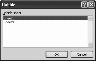
Figure 4-6. This workbook contains two hidden
worksheets. To restore one, just select it from
the list, and then click OK. Unfortunately, if you
want to show multiple hidden sheets, you have to
use the Unhide Sheet command multiple times. Excel
has no shortcut for unhiding multiple sheets at
once.
Naming and Rearranging Worksheets
The standard names
Excel assigns to new worksheetsâSheet1, Sheet2,
Sheet3, and so onâarenât very helpful for
identifying what they contain. And they become
even less helpful if you start adding new
worksheets, since the new sheet numbers donât
necessarily indicate the position of the sheets,
just the order in which you created them.
For example, if youâre on Sheet 3 and you
add a new worksheet (by choosing Home â Cells â
Insert â Insert Sheet), then the worksheet tabs
read: Sheet1, Sheet2, Sheet4, Sheet3. (Thatâs
because the Insert Sheet command inserts the new
sheet just before your current sheet.) Excel
doesnât expect you to stick with these
auto-generated names. Instead, you can rename them
by right-clicking the worksheet tab and selecting
Rename, or just double-click the sheet name.
Either way, Excel highlights the worksheet tab,
and you can type a new name directly onto the tab.
Figure
4-7 shows worksheet tabs with better
names.
Note
Excel has a small set of reserved names that
you can never use. To witness this problem, try to
create a worksheet named History. Excel doesnât
let you because it uses the History worksheet as
part of its change tracking features (Section
23.3). Use this Excel oddity to impress
your friends.
Sometimes Excel refuses to insert new
worksheets exactly where youâd like them.
Fortunately, you can easily rearrange any of your
worksheets just by dragging their tabs from one
place to another, as shown in Figure
4-8.
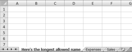
Figure 4-7. Worksheet names can be up to 31
characters long and can include letters, numbers,
some symbols, and spaces. Remember, though, the
longer the worksheet name, the fewer worksheet
tabs youâll be able to see at once, and the more
youâll need to rely on the scroll buttons to the
left of the worksheet tabs. For convenienceâs
sake, try to keep your names brief by using titles
like Sales04, Purchases, and Jet_Mileage.
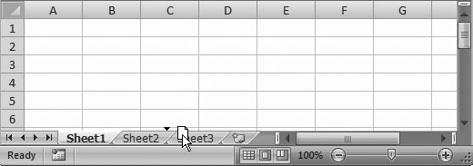
Figure 4-8. When you drag a worksheet tab, a tiny page
appears beneath the arrow cursor. As you move the
cursor around, youâll see a black triangle appear,
indicating where the worksheet will land when you
release the mouse button.
Tip
You can use a similar technique to create
copies of a worksheet. Click
the worksheet tab and begin dragging, just as you
would to move the worksheet. However, before
releasing the mouse button, press the Ctrl key
(youâll see a plus sign [+] appear). When you let
go, Excel creates a copy of the worksheet in the
new location. The original worksheet remains in
its original location. Excel gives the new
worksheet a name with a number in parentheses. For
example, a copy of Sheet1 is named Sheet1 (2). As
with any other worksheet tab, you can change this
name.
Grouping Sheets
As youâve
seen in previous chapters, Excel lets you work
with more than one column, row, or cell at a time.
The same holds true for worksheets.
You can select multiple worksheets and perform an
operation on all of them at once. This process of
selecting multiple sheets is called
grouping,
and itâs helpful if you need to hide or format
several worksheets (for example, if you want to
make sure all your worksheets start with a bright
yellow first row), and you donât want the hassle
of selecting them one at a time. Grouping
sheets doesnât let you do anything you couldnât do
ordinarilyâitâs just a nifty timesaver.
Here are some operationsâall of which are
explained in detail belowâthat you can
simultaneously perform on worksheets
that are grouped together:
-
Move, copy, delete, or hide the worksheets.
-
Apply formatting to individual cells,
columns, rows, or even entire worksheets. -
Enter new text, change text, or clear
cells. -
Cut, copy, and paste cells.
-
Adjust some page layout options, like paper
orientation (on the Page Layout tab). -
Adjust some view options, like gridlines and
the zoom level (on the View tab).
To group worksheets, hold down Ctrl while
clicking multiple worksheet tabs. When youâre
finished making your selections, release the Ctrl
key. Figure 4-9 shows an example.
![In this example, Sheet2 and Sheet3 are grouped. When worksheets are grouped, their tab colors change from gray to white. Also, in workbooks with groups, the title bar of the Excel window includes the word [Group] at the end of the file name.](https://www.oreilly.com/api/v2/epubs/0596527594/files/httpatomoreillycomsourceoreillyimages187926.jpg)
Figure 4-9. In this example, Sheet2 and Sheet3 are
grouped. When worksheets are grouped, their tab
colors change from gray to white. Also, in
workbooks with groups, the title bar of the Excel
window includes the word [Group] at the end of the
file name.
Tip
As a shortcut, you can select all the
worksheets in a workbook by right-clicking any tab
and choosing Select All Sheets.
To ungroup worksheets, right-click one of
the worksheet tabs and select Ungroup Sheets, or
just click one of the worksheet tabs that isnât in
your group. You can also remove a single worksheet
from a group by clicking it while holding down
Ctrl. However, this technique works only if the
worksheet you want to remove from the group is
not the currently active
worksheet.
Moving, copying,
deleting, or hiding grouped worksheets
As your workbook
grows,
youâll often need better ways to manage the
collection of worksheets
youâve accumulated. For example, you might want to
temporarily hide a number of worksheets,
or move a less important batch of worksheets
from the front (that is, the left side) of the
worksheet tab holder to the end (the right side).
And if a workbookâs got way too many worksheets,
you might even want to relocate several worksheets
to a brand new workbook.
Itâs easy to
perform an action on a group of worksheets. For
example, when you have a group of worksheets
selected, you can drag them en masse from one
location to another in the worksheet tab holder.
To delete or hide a group of sheets, just
right-click one of the worksheet tabs in your
group, and then choose Delete or Hide. Excel then
deletes or hides all the
selected worksheets (provided that action will
leave at least one visible worksheet in your
workbook).
Formatting cells,
columns, and rows in grouped worksheets
When you format
cells inside one grouped
worksheet, it triggers the same changes in the
cells in the other grouped
worksheets. So you have another tool you can use
to apply consistent formatting
over a batch of worksheets. Itâs mainly useful
when your worksheets are all structured in the
same way.
For example, imagine youâve
created a workbook with 10 worksheets, each one
representing a different customer order. If you
group all 10 worksheets together, and then format
just the first one, Excel formats all the
worksheets in exactly the same way. Or say you
group Sheet1 and Sheet2, and then change the font
of column B in Sheet2âExcel automatically changes
the font in column B in Sheet1, too. The same is
true if you change the formatting
of individual cells or the entire worksheetâExcel
replicates these changes across the group. (To
change the font in the currently selected cells,
just select the column and, in the Home â Font
section of the ribbon, make a new font choice from
the font list. Youâll learn much more about the
different types of formatting
you can apply to cells in Chapter
5.)
Note
It doesnât matter which worksheet you modify
in a group. For example, if Sheet1 and Sheet2 are
grouped, you can modify the formatting in either
worksheet. Excel automatically applies the changes
to the other sheet.
Entering data or changing cells in grouped
worksheets
With
grouped worksheets, you can also modify the
contents of individual cells, including entering
or changing text and clearing cell contents. For
example, if you enter a new value in cell B4 in
Sheet2, Excel enters the same value into cell B4
in the grouped Sheet1. Even more interesting, if
you modify a value in a cell in Sheet2, the same
value appears in the same cell in Sheet1, even if
Sheet1 didnât previously have a value in that
cell. Similar behavior occurs when you delete
cells.
Editing a group of worksheets
at once isnât as useful as moving and formatting
them, but it does have its moments. Once again, it
makes most sense when all the worksheets
have the same structure. For example, you could
use this technique to put the same copyright
message in cell A1 on every worksheet; or, to add
the same column titles to multiple tables
(assuming theyâre arranged in
exactly the same way).
Warning
Be careful to remember the magnified power
your keystrokes possess when youâre operating on
grouped
worksheets. For example, imagine that you move to
cell A3 on Sheet1, which happens to be empty. If
you click Delete, you see no change. However, if
cell A3 contains data on other worksheets that are
grouped, these cells are now empty. Grouper
beware.
Cutting, copying,
and pasting cells in grouped worksheets
Cut and paste
operations work the same way as entering or
modifying grouped cells. Whatever action you
perform on one grouped sheet, Excel also performs
on other grouped sheets. For example, consider
what happens if youâve grouped together Sheet1 and
Sheet2, and you copy cell A1 to A2 in Sheet1. The
same action takes place in Sheet2âin other words,
the contents of cell A1 (in Sheet2) is copied to
cell A2 (also in Sheet2). Obviously, Sheet1 and
Sheet2 might have different content in cell A1 and
A2âthe grouping
simply means that whatever was in cell A1 will now
also be in cell A2.
Adjusting printing and display options in
grouped worksheets
Excel keeps
track of printing and display settings on a
per-worksheet basis. In other words, when you set
the zoom percentage (Section
7.1.1) to 50% in one worksheet so you can
see more data, it doesnât affect the zoom in
another worksheet. However, when you make the
change for a group of
worksheets, theyâre all affected in the same
way.
Moving Worksheets from One Workbook to
Another
Once you
get the hang of creating different worksheets for
different types of information, your Excel files
can quickly fill up with more sheets than a linens
store. What happens when you want to shift some of
these worksheets around? For instance, you may
want to move (or copy) a worksheet from one Excel
file to another. Hereâs how:
-
Open both spreadsheet
files in Excel.The file that contains the worksheet you
want to move or copy is called the
source file; the other file
(where you want to move or copy the worksheet to)
is known as the destination
file. -
Go to the source
workbook.Remember, you can move from one window to
another using the Windows task bar, or by choosing
the fileâs name from the ribbonâs View â Windows â
Switch Windows list. -
Right-click the worksheet
you want to transfer, and then, from the shortcut
menu that appears, choose Move or
Copy.If you want, you can transfer multiple
worksheets at once. Just hold down the Ctrl key,
and select all the worksheets you want to move or
copy. Excel highlights all the worksheets you
select (and groups them together). Right-click the
selection, and then choose Move or Copy.When you choose Move or Copy, the âMove or
Copyâ dialog box appears (as shown in Figure
4-10).
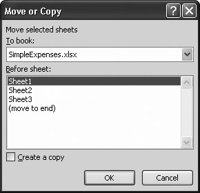
Figure 4-10. Here, the selected worksheet is about to be
moved into the SimpleExpenses.xlsx workbook. (The
source workbook isnât shown.) The SimpleExpenses
workbook already contains three worksheets (named
Sheet1, Sheet2, and Sheet3). Excel inserts the new
worksheet just before the first sheet. Because the
âCreate a copyâ checkbox isnât turned on, Excel
removes the worksheet from the source workbook
when it completes the transfer. -
Choose the destination
file from the âTo bookâ list.The âTo bookâ drop-down list shows all the
currently open workbooks (including the source
workbook).Tip
Excel also lets you move your worksheets to
a new workbook, which it automatically creates for
you. To move them, choose the â(new book)â item in
the âTo bookâ list. The new workbook wonât have
the standard three worksheets. Instead, itâll have
only the worksheets youâve transferred. -
Specify the position where
you want the worksheet inserted.Choose a destination worksheet from the
âBefore sheetâ list. Excel places the copied
worksheets just before the
worksheet you select. If you want to place the
worksheets at the end of the destination workbook,
select â(move to end).â Of course, you can always
rearrange the worksheets after you transfer them,
so you donât need to worry too much about getting
the perfect placement. -
If you want to copy the
worksheet, turn on the âCreate a copyâ checkbox at
the bottom of the window.If you donât turn this option on, then Excel
copies the worksheet to the destination workbook
and remove it from the current workbook. If you
do turn this option on,
youâll end up with a copy of the workbook in both
places. -
Click
OK.This final step closes the âMove or Copyâ
dialog box and transfers the worksheet (or
worksheets).
Note
If there are any worksheet name conflicts,
Excel adds a number in parentheses after the moved
sheetâs name. For example, if you try to copy a
worksheet named Sheet1 to a workbook that already
has a Sheet1, Excel names the copied worksheet
Sheet1 (2).
Find and Replace
When youâre dealing
with great mounds of information, you may have a
tough time ferreting out the nuggets of data you
need. Fortunately, Excelâs find feature is great
for helping you locate numbers or text, even when
theyâre buried within massive workbooks holding
dozens of worksheets. And if you need to make
changes to a bunch of identical items, the
find-and-replace option can be a real
timesaver.
The âFind and Replaceâ feature includes both
simple and advanced options. In its basic version,
youâre only a quick keystroke combo away from a
word or number you know is
lurking somewhere in your data pile. With the
advanced options turned on, you can do things like
search for cells that have certain formatting
characteristics and apply changes automatically.
The next few sections dissect these
features.
The Basic Find
Excelâs find feature is a
little like the Go To tool described in Chapter 1,
which lets you move across a large expanse of
cells in a single bound. The difference is that Go
To moves to a known location,
using the cell address you specify. The find
feature, on the other hand, searches every cell
until it finds the content youâve asked Excel to
look for. Excelâs search works similarly to the
search feature in Microsoft Word, but itâs worth
keeping in mind a few additional details:
-
Excel searches by comparing the content you
enter with the content in each cell. For example,
if you searched for the word
Date, Excel identifies as a
match a cell containing the phrase Date
Purchased. -
When searching cells that contain numeric or
date information, Excel always searches the
display text.
(For more information about the difference between
the way Excel displays a numeric valueâthe
underlying value Excel actually
storesâsee Section
2.1.)For example, say a cell displays dates using
the day-month-year format, like
2-Dec-05. You can find this
particular cell by searching for any part of the
displayed date (using search strings like
Dec or 2-Dec-05). But if you
use the search string
12/2/2005, you wonât find a
match because the search string and the display
text are different. A similar behavior occurs with
numbers. For example, the search strings
$3 and
3.00 match the currency value
$3.00. However, the search
string 3.000 wonât turn up
anything because Excel wonât be able to make a
full text match. -
Excel searches one cell at a time, from
left-to-right. When it reaches the end of a row,
it moves to the first column of the next
row.
To perform a find
operation, follow these steps:
-
Move to the cell where you
want the search to begin.If you start off halfway down the worksheet,
for example, the search covers the cells from
there to the end of the worksheet, and then âloops
overâ and starts at cell A1. If you select a group
of cells, Excel restricts the search to just those
cells. You can search across a set of columns,
rows, or even a non-contiguous group of
cells. -
Choose Home â Editing â
Find & Select â Find, or press
Ctrl+F.The «Find and Replaceâ
window appears, with the Find tab selected.Note
To assist frequent searches, Excel lets you
keep the Find and Replace window hanging around
(rather than forcing you to use it or close it, as
is the case with many other dialog boxes). You can
continue to move from cell to cell and edit your
worksheet data even while the âFind and Replaceâ
window remains visible. -
In the âFind whatâ combo
box, enter the word, phrase, or number youâre
looking for.If youâve performed other searches recently,
you can reuse these search terms. Just choose the
appropriate search text from the âFind whatâ
drop-down list. -
Click Find
Next.Excel jumps to the next matching cell, which
becomes the active cell. However, Excel doesnât
highlight the matched text or in any way indicate
why it decided the cell was a
match. (Thatâs a bummer if youâve got, say, 200
words crammed into a cell.) If it doesnât find a
matching cell, Excel displays a message box
telling you it couldnât find the requested
content.If the first match isnât what youâre looking
for, you can keep looking by clicking Find Next
again to move to the next match. Keep clicking
Find Next to move through the worksheet. When you
reach the end, Excel resumes the search at the
beginning of your worksheet, potentially bringing
you back to a match youâve already seen. When
youâre finished with the search, click Close to
get rid of the âFind and Replaceâ window.
Find All
One of the problems
with searching in Excel is that youâre never quite
sure how many matches there are in a worksheet.
Sure, clicking Find Next gets you from one cell to
the next, but wouldnât it be easier for Excel to
let you know right away how many matches it
found?
Enter the Find All feature. With Find All,
Excel searches the entire worksheet in one go, and
compiles a list of matches, as shown in Figure
4-11.
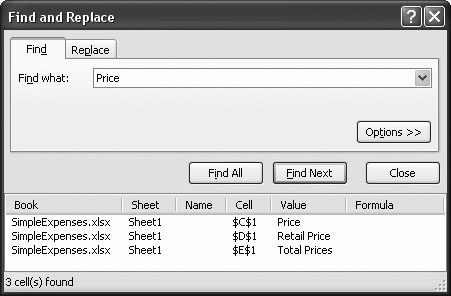
Figure 4-11. In the example shown here, the search for
âPriceâ matched three cells in the worksheet. The
list shows you the complete text in the matching
cell and the cell reference (for example, $C$1,
which is a reference to cell C1).
The Find All button doesnât lead you through
the worksheet like the find feature. Itâs up
to you to select one of the results in the list,
at which point Excel automatically moves you to
the matching cell.
The Find All list wonât automatically
refresh itself: After youâve run a Find All
search, if you add new data
to your worksheet, you need to run a new search to
find any newly added terms. However, Excel does
keep the text and numbers in your found-items list
synchronized with any changes you make in the
worksheet. For example, if you change cell D5 to
Total Price, the change appears in the Value
column in the found-items list
automatically. This tool is
great for editing a worksheet because you can keep
track of multiple changes at a single
glance.
Finally, the Find All feature is the heart
of another great Excel guru trick: it gives you
another way to change multiple cells at once.
After youâve performed the Find All search, select
all the entries you want to change from the list
by clicking them while you hold down Ctrl (this
trick allows you to select several at once). Click
in the formula bar, and then start typing the new
value. When youâre finished, hit Ctrl+Enter to
apply your changes to every selected cell.
Voilà âitâs like «Find and Replaceâ,
but youâre in control!
More Advanced Searches
Basic searches are fine if all you need to
find is a glaringly
unique phrase or number (Pet Snail
Names or
10,987,654,321). But Excelâs
advanced search feature gives you lots of ways to
fine-tune your searches or even search more than
one worksheet. To conduct an advanced search,
begin by clicking the «Find and Replaceâ
windowâs Options
button, as shown in Figure
4-12.
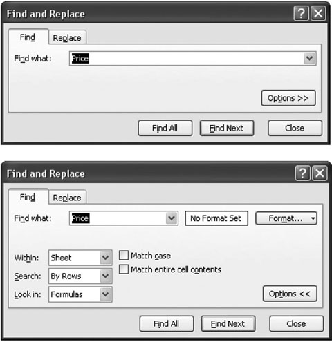
Figure 4-12. In the standard âFind and Replaceâ window
(top), when you click Options, Excel gives you a
slew of additional settings (bottom) so you can
configure things like search direction, case
sensitivity, and format matching.
You can set any or all of the following
options:
-
If you want your search to span multiple
worksheets, go to the Within box, and then choose
Workbook. The standard option, Sheet, searches all
the cells in the currently active worksheet. If
you want to continue the search in the other
worksheets in your workbook, choose Workbook.
Excel examines the worksheets from left to right.
When it finishes searching the last
worksheet, it loops back and starts examining the
first worksheet. -
The Search pop-up menu lets you choose the
direction you want to search. The standard option,
By Rows, completely searches each row before
moving on to the next one. That means that if you
start in cell B2, Excel searches C2, D2, E2, and
so on. Once itâs moved through every column in the
second row, it moves onto the third row and
searches from left to right.On the other hand, if you choose By Columns,
Excel searches all the rows in the current column
before moving to the next column. That means that
if you start in cell B2, Excel searches B3, B4,
and so on until it reaches the bottom of the
column and then starts at the top of the next
column (column C).Note
The search direction determines which path
Excel follows when itâs searching. However, the
search will still ultimately traverse every cell
in your worksheet (or the current
selection). -
The «Match caseâ option
lets you specify whether capitalization is
important. If you select âMatch caseâ, Excel
finds only words or
phrases whose capitalization matches. Thus,
searching for Date matches
the cell value Date, but not
date. -
The âMatch entire cell contentsâ option lets
you restrict your searches to the entire contents
of a cell. Excel ordinarily looks to see if your
search term is contained
anywhere inside a cell. So,
if you specify the word
Price, Excel finds cells
containing text like Current
Price and even Repriced
Items. Similarly, numbers like 32 match
cell values like 3253, 10032, and 1.321. Turning
on the âMatch entire cell contentsâ option forces
Excel to be precise.
Note
Remember, Excel searches for numbers as
theyâre displayed (as opposed
to looking at the underlying values that Excel
uses to store numbers internally). That means that
if youâre searching for a number formatted using
the dollar Currency format ($32.00, for example),
and youâve turned on the âMatch entire cell
contentsâ checkbox, youâll need to enter the
number exactly as it appears on the worksheet.
Thus, $32.00 would work, but 32 alone wonât help
you.
Finding Formatted Cells
Excelâs «Find and Replaceâ is
an equal opportunity search tool: It doesnât care
what the contents of a cell look like. But what if
you know, for example, that the data youâre
looking for is formatted in bold, or that itâs a
number that uses the Currency format? You can use
these formatting details to
help Excel find the data you want and ignore cells
that arenât relevant.
To use formatting details as part of your
search criteria, follow these steps:
-
Launch the Find
tool.Choose Home â Editing â Find & Select â
Find, or press Ctrl+F. Make sure that the
«Find and Replaceâ
window is showing the advanced options (by
clicking the Options button). -
Click the Format button
next to the âFind whatâ search
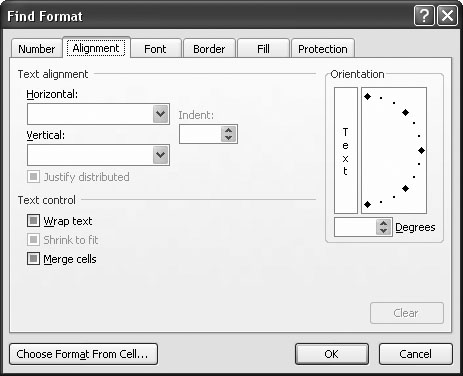
box.The Find Format dialog box appears (Figure
4-13). It contains the same options as the
Format Cells dialog box discussed in Section
5.1.
Figure 4-13. In the Find Format dialog box, Excel wonât
use any formatting option thatâs blank or grayed
out as part of itâs search criteria. For example,
here, Excel wonât search based on alignment.
Checkboxes are a little trickier. In some versions
of Windows, it looks like the checkbox is filled
with a solid square (as with the âMerge cellsâ
setting in this example). In other versions of
Windows, it looks like the checkbox is dimmed and
checked at the same time. Either way, this visual
cue indicates that Excel wonât use the setting as
part of its search. -
Specify the format
settings you want to look for.Using the Find Format dialog box, you can
specify any combination of number format,
alignment, font, fill pattern, borders, and
formatting. Chapter 5 explains all these formatting
settings in detail. You can also search for
protected and locked cells, which are described in
Chapter
16. -
When youâre finished,
click OK to return to the âFind and Replaceâ
window.Next to the âFind whatâ search box, a
preview appears indicating the formatting of the
cell that youâll be searching for, as shown in
Figure
4-14.To remove these formatting restrictions,
click the pop-up menu to the right of the Format
button and then choose Clear Find.
Tip
Rather than specifying all the format
settings manually, you can copy them from another
cell. Just click the Choose Format From Cell
button at the bottom of the Find Format dialog
box. The pointer changes to a plus symbol with an
eyedropper next to it. Next, click any cell that
has the formatting you want to match. Keep in mind
that when you use this approach, you copy
all the format
settings.
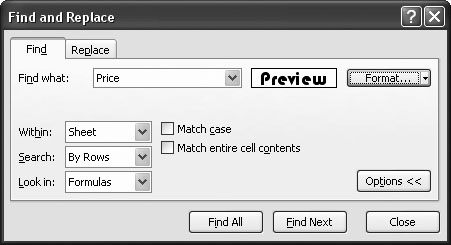
Figure 4-14. The Find Format
dialog box shows a basic preview of your
formatting choices. In this example, the search
will find cells containing the word âpriceâ that
also use white lettering, a black background, and
the Bauhaus font.
Finding and Replacing Values
You can use Excelâs search muscles to find
not only the information youâre interested in, but
also to modify cells quickly and easily. Excel
lets you make two types of changes using its
replace tool:
-
You can automatically
change cell content. For example, you
can replace the word Colour
with Color or the number
$400 with
$40. -
You can automatically
change cell formatting. For example,
you can search for every cell that contains the
word Price or the number
$400 and change the fill
color. Or, you can search for every cell that uses
a specific font, and modify these cells so they
use a new font.
Hereâs how to perform a replace operation.
The box below gives some superhandy tricks you can
do with this process.
-
Move to the cell where the
search should begin.Remember, if you donât want to search the
entire spreadsheet, just select the range of cells
you want to search. -
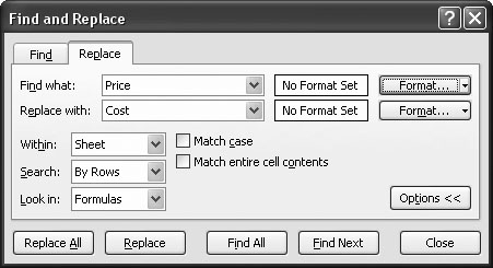
Choose Home â Editing â
Find & Select â Replace, or press
Ctrl+H.The âFind and Replaceâ window appears, with
the Replace tab selected, as shown in Figure
4-15.
Figure 4-15. The Replace tab looks pretty similar to the
Find tab. Even the advanced options are the same.
The only difference is that you also need to
specify the text you want to use as a replacement
for the search terms you find. -
In the âFind whatâ box,
enter your search term. In the âReplace withâ box,
enter the replacement text.Type the replacement text exactly as you
want it to appear. If you want to set any advanced
options, click the Options button (see the earlier
sections âMore Advanced Searchesâ and âFinding
Formatted Cellsâ for more on your choices). -
Perform the
search.Youâve got four different options here.
Replace All immediately
changes all the matches your search identifies.
Replace changes only the
first matched item (you can then click Replace
again to move on to subsequent matches or to
select any of the other three options).
Find All works just like the
same feature described in the box in Section
4.2.5. Find Next moves
to the next match, where you can click Replace to
apply your specified change, or click any of the
other three buttons. The replace options are good
if youâre confident you want to make a change; the
find options work well if you first want to see
what changes youâre about to make (although you
can reverse either option using Ctrl+Z to fire off
the Undo command).
Note
Itâs possible for a single cell to contain
more than one match. In this case, clicking
Replace replaces every occurrence of that text in
the entire cell.
Spell Check
A spell
checker in Excel? Is that supposed to be for
people who canât spell 138 correctly? The fact is
that more and more people are cramming textâcolumn
headers, boxes of commentary, lists of favorite
cereal combinationsâinto their spreadsheets. And
Excelâs designers have graciously responded by
providing the very same spell checker that youâve
probably used with Microsoft Word. As you might
expect, Excelâs spell checker examines only text
as it sniffs its way through a spreadsheet.
Note
The same spell checker works in almost every
Office application, including Word, PowerPoint,
and Outlook.
To start the spell checker, follow these
simple steps:
-
Move to where you want to
start the spell check.If you want to check the entire worksheet
from start to finish, move to the first cell.
Otherwise, move to the location where you want to
start checking. Or, if you want to check a portion
of the worksheet, select the cells you want to
check.Unlike the âFind and Replaceâ feature,
Excelâs spell check can check only one worksheet
at a time. -
Choose Review â Proofing â
Spelling, or press F7.The Excel spell checker starts working
immediately, starting with the current cell and
moving to the right, going from column to column.
After it finishes the last column of the current
row, checking continues with the first column of
the next row.If you donât start at the first cell (A1) in
your worksheet, Excel asks you when it reaches the
end of the worksheet whether it should continue
checking from the beginning of the sheet. If you
say yes, it checks the remaining cells and stops
when it reaches your starting point (having made a
complete pass through all of your cells).
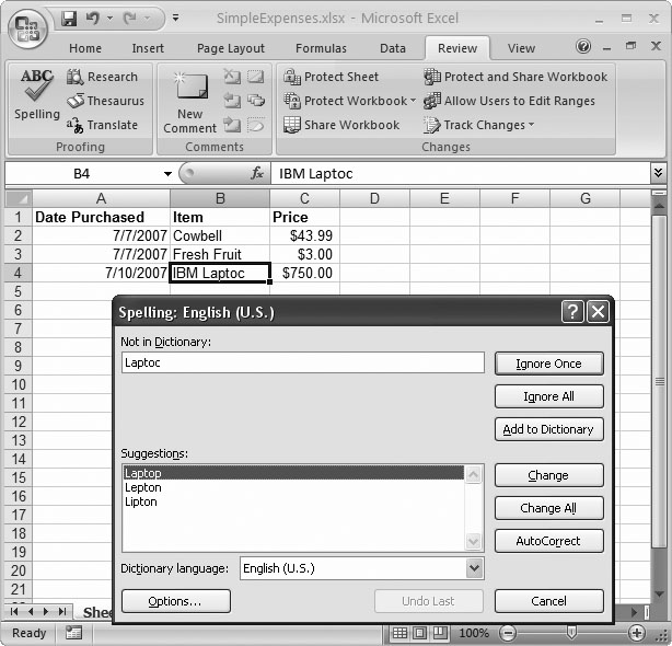
When the spell check finishes, a dialog box
informs you that all cells have been checked. If
your cells pass the spell check, this dialog box
is the only feedback you receive. On the other
hand, if Excel discovers any potential spelling
errors during its check, it displays a Spelling
window, as shown in Figure
4-16, showing the offending word and a list
of suggestions.
The Spelling window offers a wide range of
choices. If you want to use the list of
suggestions to perform a correction, you have
three options:
-
Click one of the words in the list of
suggestions, and then click Change to replace your
text with the proper spelling. Double-clicking the
word has the same effect.
Figure 4-16. When Excel
encounters a word it thinks is misspelled, it
displays the Spelling window. The cell containing
the wordâbut not the actual word itselfâgets
highlighted with a black border. Excel doesnât let
you edit your file while the Spelling window is
active. You either have to click one of the
options on the Spelling window or cancel the spell
check. -
Click one of the words in the list of
suggestions, and click Change All to replace your
text with the proper spelling. If Excel finds the
same mistake elsewhere in your worksheet, it
repeats the change automatically. -
Click one of the words in the list of
suggestions, and click AutoCorrect. Excel makes
the change for this cell, and for any other
similarly misspelled words. In addition, Excel
adds the correction to its AutoCorrect list
(described in Section
2.2.2). That means if you type the same
unrecognized word into another cell (or even
another workbook), Excel automatically corrects
your entry. This option is useful if youâve
discovered a mistake that you frequently
make.
Tip
If Excel spots an error but it doesnât give
you the correct spelling in its list of
suggestions, just type the correction into the
âNot in Dictionaryâ box and hit Enter. Excel
inserts your correction into the corresponding
cell.
On the other hand, if Excel is warning you
about a word that doesnât represent a mistake
(like your company name or some specialized term),
you can click one of the following buttons:
-
Ignore
Once skips the word and continues the
spell check. If the same word appears elsewhere in
your spreadsheet, Excel prompts you again to make
a correction. -
Ignore All
skips the current word and all other instances of
that word throughout your spreadsheet. You might
use Ignore All to force Excel to disregard
something you donât want to correct, like a
personâs name. The nice thing about Ignore All is
that Excel doesnât prompt you again if it finds
the same name, but it does prompt you again if it
finds a different spelling (for example, if you
misspelled the name). -
Add
to Dictionary adds the word to Excelâs
custom dictionary.
Adding a word is great if you plan to keep using a
word thatâs not in Excelâs dictionary. (For
example, a company name makes a good addition to
the custom dictionary.) Not only does Excel ignore
any occurrences of this word, but if it finds a
similar but slightly different variation of that
word, it provides the custom word in its list of
suggestions. Even better, Excel uses the custom
dictionary in every workbook you spell
check. -
Cancel stops
the operation altogether. You can then correct the
cell manually (or do nothing) and resume the spell
check later.
Spell Checking Options
Excel lets you tweak how the spell checker works
by letting you change a few basic options that
control things like the language used and which,
if any, custom dictionaries Excel examines. To set
these options (or just to take a look at them),
choose Office button â Excel Options, and then
select the Proofing section (Figure
4-17).
You can also reach these options by clicking
the Spelling windowâs Options button while a spell
check is underway.
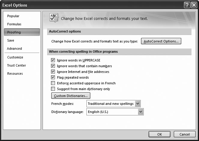
Figure 4-17. The spell checker
options allow you to specify the language and a
few other miscellaneous settings. This figure
shows the standard settings that Excel uses when
you first install it.
The most important spell check setting is
the language (at the bottom of the window), which
determines what dictionary
Excel uses. Depending on the version of Excel that
youâre using and the choices you made while
installing the software, you might be using one or
more languages during a spell check
operation.
Some of the other spelling options you can
set include:
-
Ignore words in
UPPERCASE. If you choose this option,
Excel wonât bother checking any word written in
all capitals (which is helpful when your text
contains lots of acronyms). -
Ignore words that contain
numbers. If you choose this option,
Excel wonât check words that contain numeric
characters, like Sales43 or
H3ll0. If you donât choose
this option, then Excel flags these entries as
errors unless youâve specifically added them to
the custom dictionary. -
Ignore Internet and file
addresses. If you choose this option,
Excel ignores words that appear to be file paths
(like C:Documents and
Settings) or Web site addresses (like
http://FreeSweatSocks.com). -
Flag repeated
words. If you choose this option, Excel
treats words that appear consecutively (âthe theâ)
as an error. -
Suggest from main
dictionary only. If you choose this
option, the spell
checker doesnât suggest words from the custom
dictionary. However, it still
accepts a word that matches
one of the custom dictionary entries.
You can also choose the file Excel uses to
store custom wordsâthe unrecognized words that you
add to the dictionary while a spell check is
underway. Excel automatically creates a file named
custom.dic
for you to use, but you might want to use another
file if youâre sharing someone elseâs custom
dictionary. (You can use more than one custom
dictionary at a time. If you do, Excel combines
them all to get one list of custom words.) Or, you
might want to edit the list of words if youâve
mistakenly added something that shouldnât be
there.
To perform any of these tasks, click the
Custom Dictionaries button, which opens the Custom
Dictionaries dialog box (Figure
4-18). From this dialog box, you can remove
your custom dictionary, change it, or add a new
one.
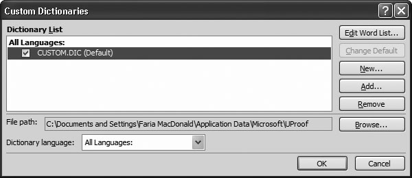
Figure 4-18. Excel starts you off with a custom
dictionary named custom.dic (shown here). To add
an existing custom dictionary, click Add and
browse to the file. Or, click New to create a new,
blank custom dictionary. You can also edit the
list of words a dictionary contains (select it and
click Edit Word List). Figure
4-19 shows an example of dictionary
editing.
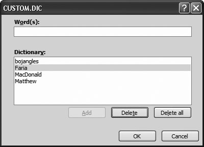
Figure 4-19. This custom dictionary is fairly modest. It
contains three names and an unusual word. Excel
lists the words in alphabetical order. You can add
a new word directly from this window (type in the
text and click Add), remove one (select it and
click Delete), or go nuclear and remove them all
(click Delete All).
Note
All custom dictionaries are ordinary text
files with the extension .dic. Unless you tell it
otherwise, Excel assumes that custom dictionaries
are located in the Application
DataMicrosoftUProof folder in the
folder Windows uses for user-specific settings.
For example, if youâre logged in under the user
account Brad_Pitt, youâd find the custom
dictionary in the C:Documents and
SettingsBrad_PittApplication
DataMicrosoftUProof folder.
Get Excel 2007: The Missing Manual now with the O’Reilly learning platform.
O’Reilly members experience books, live events, courses curated by job role, and more from O’Reilly and nearly 200 top publishers.
It is important that you know how to effectively manage your worksheets. By default, three worksheets appear in each new workbook. In this lesson, you will learn how to name, add, delete, group, and ungroup worksheets. Additionally, you will learn how to freeze specific parts of the worksheet so they are always visible.

Naming Worksheets
When you open an Excel workbook, there are three sheets by default and the default name on the tabs are Sheet1, Sheet2 and Sheet3. These are not very informative names. Excel 2007 allows you to define a meaningful name for each worksheet in a workbook so you can quickly locate information.
To Name a Worksheet:
- Right-click the sheet tab to select it.
- Choose Rename from the menu that appears. The text is highlighted by a black box.

- Type a new name for the worksheet.

- Click off the tab. The worksheet now assumes the descriptive name defined.
OR - Click the Format command in the Cells group on the Home tab.
- Select Rename Sheet. The text is highlighted by a black box.
- Type a new name for the worksheet.
- Click off the tab. The worksheet now assumes the descriptive name defined.
Inserting Worksheets
You can change the default number of sheets that appear by clicking the Microsoft Office Button and choosingExcel Options. You also have the ability to insert new worksheets if needed, while you are working.
To Insert a New Worksheet:
- Left-click the Insert Worksheet icon. A new sheet will appear. It will be named Sheet4, Sheet5 or whatever the next sequential sheet number may be in the workbook.

- Press the Shift and the F11 keys on your keyboard.
OR
Deleting Worksheets
Any worksheet can be deleted from a workbook, including those that have data in it. Remember, a workbook must contain at least one worksheet.
To Delete One or More Worksheets:
- Click on the sheet(s) you want to delete.
- Right-click the sheet(s) and a menu appears.
- Select Delete.

- Select the sheet you want to remove.
- Click the drop-down arrow next to Delete in the Cells group on the Home tab.
- From the menu that appears, select Delete Sheet.
OR
Grouping and Ungrouping Worksheets
A workbook is a multi-page Excel document that contains multiple worksheets. Sometimes you will want to work with the worksheets one at a time as if each is a single unit. Other times, the same information or formatting may need to be added to every worksheet.
Worksheets can be combined together into a group. Grouping worksheets allows you to apply identical formulas and/or formatting across all the worksheets in the group. When you group worksheets, any changes made to one worksheet will also be changed in any other worksheets in the group.
To Group Contiguous Worksheets:
- Select the first sheet you want to group.
- Press and hold the Shift key on your keyboard.
- Click the last sheet you want to group.

- Release the Shift key.
- The sheets are now grouped. All the sheets between the first sheet and last sheet selected are part of the group. The sheet tabs will appear white for the grouped sheets.

- Make any changes to one sheet and the changes will appear in all the grouped sheets.
To Group Non-Contiguous Sheets:
- Select the first sheet you want to group.
- Press and hold the Ctrl key on your keyboard.
- Click the next sheet you want to group.
- Continuing clicking the sheets you want to group.
- Release the Control key.
- The sheets are now grouped. The sheet tabs will appear white for the grouped sheets. Only the sheets selected are part of the group.
- Make any changes to one sheet and the changes will appear in all the grouped sheets.
To Ungroup Worksheets:
- Right-click one of the sheets.
- Select Ungroup from the list.
Freezing Worksheet Panes
The ability to freeze, or lock, specific rows or columns in your spreadsheet is a really useful feature in Excel. It is called freezing panes. When you freeze panes, you select rows or columns that will remain visible all the time, even as you are scrolling. This is particularly useful when working with large spreadsheets.
To Freeze a Row:
- Select the row below the one that you want frozen. For example, if you want row 1 & 2 to appear at the top even as you scroll, then select row 3.

- Click the View tab.
- Click the Freeze Pane command in the Window group.

- Choose Freeze Panes. A thin, black line appears below everything that is frozen in place.

- Scroll down in the worksheet to see the pinned rows.
To Unfreeze a Pane:
- Click the Freeze Pane command.
- Select the Unfreeze command.
To Freeze a Column:
- Select the column to the right of the column(s) you want frozen. For example, if you want columns A & B to always appear on the left, just select column C.
- Click the View tab.
- Click the Freeze Pane command in the Window group.
- Choose Freeze Pane. A thin, black line appears to the right of the frozen area.
- Scroll across in the worksheet to see the pinned columns.
На чтение 16 мин. Просмотров 14.8k.
Malcolm Gladwell
Мечтатель начинает с чистого листа бумаги и переосмысливает мир
Эта статья содержит полное руководство по использованию Excel
VBA Worksheet в Excel VBA. Если вы хотите узнать, как что-то сделать быстро, ознакомьтесь с кратким руководством к рабочему листу VBA ниже.
Если вы новичок в VBA, то эта статья — отличное место для начала. Мне нравится разбивать вещи на простые термины и объяснять их на простом языке.
Вы можете прочитать статью от начала до конца, так как она написана в логическом порядке. Или, если предпочитаете, вы можете использовать оглавление ниже и перейти непосредственно к теме по вашему выбору.
Содержание
- Краткое руководство к рабочему листу VBA
- Вступление
- Доступ к рабочему листу
- Использование индекса для доступа к рабочему листу
- Использование кодового имени рабочего листа
- Активный лист
- Объявление объекта листа
- Доступ к рабочему листу в двух словах
- Добавить рабочий лист
- Удалить рабочий лист
- Цикл по рабочим листам
- Использование коллекции листов
- Заключение
Краткое руководство к рабочему листу VBA
В следующей таблице приведен краткий обзор различных методов
Worksheet .
Примечание. Я использую Worksheet в таблице ниже, не указывая рабочую книгу, т.е. Worksheets, а не ThisWorkbook.Worksheets, wk.Worksheets и т.д. Это сделано для того, чтобы примеры были понятными и удобными для чтения. Вы должны всегда указывать рабочую книгу при использовании Worksheets . В противном случае активная рабочая книга будет использоваться по умолчанию.
| Задача | Исполнение |
| Доступ к рабочему листу по имени |
Worksheets(«Лист1») |
| Доступ к рабочему листу по позиции слева |
Worksheets(2) Worksheets(4) |
| Получите доступ к самому левому рабочему листу |
Worksheets(1) |
| Получите доступ к самому правому листу |
Worksheets(Worksheets.Count) |
| Доступ с использованием кодового имени листа (только текущая книга) |
Смотри раздел статьи Использование кодового имени |
| Доступ по кодовому имени рабочего листа (другая рабочая книга) |
Смотри раздел статьи Использование кодового имени |
| Доступ к активному листу | ActiveSheet |
| Объявить переменную листа | Dim sh As Worksheet |
| Назначить переменную листа | Set sh = Worksheets(«Лист1») |
| Добавить лист | Worksheets.Add |
| Добавить рабочий лист и назначить переменную |
Worksheets.Add Before:= Worksheets(1) |
| Добавить лист в первую позицию (слева) |
Set sh =Worksheets.Add |
| Добавить лист в последнюю позицию (справа) |
Worksheets.Add after:=Worksheets(Worksheets.Count) |
| Добавить несколько листов | Worksheets.Add Count:=3 |
| Активировать рабочий лист | sh.Activate |
| Копировать лист | sh.Copy |
| Копировать после листа | sh1.Copy After:=Sh2 |
| Скопировать перед листом | sh1.Copy Before:=Sh2 |
| Удалить рабочий лист | sh.Delete |
| Удалить рабочий лист без предупреждения |
Application.DisplayAlerts = False sh.Delete Application.DisplayAlerts = True |
| Изменить имя листа | sh.Name = «Data» |
| Показать/скрыть лист | sh.Visible = xlSheetHidden sh.Visible = xlSheetVisible sh.Name = «Data» |
| Перебрать все листы (For) | Dim i As Long For i = 1 To Worksheets.Count Debug.Print Worksheets(i).Name Next i |
| Перебрать все листы (For Each) | Dim sh As Worksheet For Each sh In Worksheets Debug.Print sh.Name Next |
Вступление
Три наиболее важных элемента VBA — это Рабочая книга, Рабочий лист и Ячейки. Из всего кода, который вы пишете, 90% будут включать один или все из них.
Наиболее распространенное использование Worksheet в VBA для доступа к его ячейкам. Вы можете использовать его для защиты, скрытия, добавления, перемещения или копирования листа.
Тем не менее, вы будете в основном использовать его для выполнения некоторых действий с одной или несколькими ячейками на листе.
Использование Worksheets более простое, чем использование рабочих книг. С книгами вам может потребоваться открыть их, найти, в какой папке они находятся, проверить, используются ли они, и так далее. С рабочим листом он либо существует в рабочей книге, либо его нет.
Доступ к рабочему листу
В VBA каждая рабочая книга имеет коллекцию рабочих листов. В этой коллекции есть запись для каждого рабочего листа. Эта коллекция называется просто Worksheets и используется очень похоже на коллекцию Workbooks. Чтобы получить доступ к рабочему листу, достаточно указать имя.
Приведенный ниже код записывает «Привет Мир» в ячейках A1 на листах: Лист1, Лист2 и Лист3 текущей рабочей книги.
Sub ZapisVYacheiku1()

    ' Запись в ячейку А1 в листе 1, листе 2 и листе 3
    ThisWorkbook.Worksheets("Лист1").Range("A1") = "Привет Мир"
    ThisWorkbook.Worksheets("Лист2").Range("A1") = "Привет Мир"
    ThisWorkbook.Worksheets("Лист3").Range("A1") = "Привет Мир"

End Sub
Коллекция Worksheets всегда принадлежит книге. Если мы не
указываем рабочую книгу, то активная рабочая книга используется по умолчанию.
Sub ZapisVYacheiku1()

    ' Worksheets относятся к рабочим листам в активной рабочей книге.
    Worksheets("Лист1").Range("A1") = "Привет Мир"
    Worksheets("Лист2").Range("A1") = "Привет Мир"
    Worksheets("Лист3").Range("A1") = "Привет Мир"

End Sub
Скрыть рабочий лист
В следующих примерах показано, как скрыть и показать лист.
ThisWorkbook.Worksheets("Лист1").Visible = xlSheetHidden

ThisWorkbook.Worksheets("Лист1").Visible = xlSheetVisible
Если вы хотите запретить пользователю доступ к рабочему
листу, вы можете сделать его «очень скрытым». Это означает, что это может быть
сделано видимым только кодом.
' Скрыть от доступа пользователя
ThisWorkbook.Worksheets("Лист1").Visible = xlVeryHidden

' Это единственный способ сделать лист xlVeryHidden видимым
ThisWorkbook.Worksheets("Лист1").Visible = xlSheetVisible
Защитить рабочий лист
Другой пример использования Worksheet — когда вы хотите защитить его.
ThisWorkbook.Worksheets("Лист1").Protect Password:="Мойпароль"

ThisWorkbook.Worksheets("Лист1").Unprotect Password:="Мойпароль"
Индекс вне диапазона
При использовании Worksheets вы можете получить сообщение об
ошибке:
Run-time Error 9 Subscript out of Range
Это означает, что вы пытались получить доступ к рабочему листу, который не существует. Это может произойти по следующим причинам:
- Имя Worksheet , присвоенное рабочим листам, написано неправильно.
- Название листа изменилось.
- Рабочий лист был удален.
- Индекс был большим, например Вы использовали рабочие листы (5), но есть только четыре рабочих листа
- Используется неправильная рабочая книга, например Workbooks(«book1.xlsx»).Worksheets(«Лист1») вместо
Workbooks(«book3.xlsx»).Worksheets («Лист1»).
Если у вас остались проблемы, используйте один из циклов из раздела «Циклы по рабочим листам», чтобы напечатать имена всех рабочих листов коллекции.
Использование индекса для доступа к рабочему листу
До сих пор мы использовали имя листа для доступа к листу.
Указатель относится к положению вкладки листа в рабочей книге. Поскольку
положение может быть легко изменено пользователем, не рекомендуется
использовать это.
В следующем коде показаны примеры использования индекса.
' Использование этого кода является плохой идеей, так как
' позиции листа все время меняются
Sub IspIndList()

    With ThisWorkbook
        ' Самый левый лист
        Debug.Print .Worksheets(1).Name
        ' Третий лист слева
        Debug.Print .Worksheets(3).Name
        ' Самый правый лист
        Debug.Print .Worksheets(.Worksheets.Count).Name
    End With

End Sub
В приведенном выше примере я использовал Debug.Print для печати в Immediate Window. Для просмотра этого окна выберите «Вид» -> «Immediate Window » (Ctrl + G).
Использование кодового имени рабочего листа
Лучший способ получить доступ к рабочему листу —
использовать кодовое имя. Каждый лист имеет имя листа и кодовое имя. Имя листа
— это имя, которое отображается на вкладке листа в Excel.
Изменение имени листа не приводит к изменению кодового имени, что означает, что ссылка на лист по кодовому имени — отличная идея.
Если вы посмотрите в окне свойств VBE, вы увидите оба имени.
На рисунке вы можете видеть, что кодовое имя — это имя вне скобок, а имя листа
— в скобках.
Вы можете изменить как имя листа, так и кодовое имя в окне
свойств листа (см. Изображение ниже).
Если ваш код ссылается на кодовое имя, то пользователь может
изменить имя листа, и это не повлияет на ваш код. В приведенном ниже примере мы
ссылаемся на рабочий лист напрямую, используя кодовое имя.
Sub IspKodImya2()

    ' Используя кодовое имя листа
    Debug.Print CodeName.Name
    CodeName.Range("A1") = 45
    CodeName.Visible = True

End Sub
Это делает код легким для чтения и безопасным от изменения
пользователем имени листа.
Кодовое имя в других книгах
Есть один недостаток использования кодового имени. Он относится только к рабочим листам в рабочей книге, которая содержит код, т.е. ThisWorkbook.
Однако мы можем использовать простую функцию, чтобы найти
кодовое имя листа в другой книге.
Sub ИспЛист()

    Dim sh As Worksheet
    ' Получить рабочий лист под кодовым именем
    Set sh = SheetFromCodeName("CodeName", ThisWorkbook)
    ' Используйте рабочий лист
    Debug.Print sh.Name

End Sub

' Эта функция получает объект листа из кодового имени
Public Function SheetFromCodeName(Name As String, bk As Workbook) As Worksheet

    Dim sh As Worksheet
    For Each sh In bk.Worksheets
        If sh.CodeName = Name Then
           Set SheetFromCodeName = sh
           Exit For
        End If
    Next sh

End Function
Использование приведенного выше кода означает, что если
пользователь изменит имя рабочего листа, то на ваш код это не повлияет.
Существует другой способ получения имени листа внешней
рабочей книги с использованием кодового имени. Вы можете использовать элемент
VBProject этой Рабочей книги.
Вы можете увидеть, как это сделать, в примере ниже. Я включил это, как дополнительную информацию, я бы рекомендовал использовать метод из предыдущего примера, а не этот.
Public Function SheetFromCodeName2(codeName As String _
                             , bk As Workbook) As Worksheet

    ' Получить имя листа из CodeName, используя VBProject
    Dim sheetName As String
    sheetName = bk.VBProject.VBComponents(codeName).Properties("Name")

    ' Используйте имя листа, чтобы получить объект листа
    Set SheetFromCodeName2 = bk.Worksheets(sheetName)

End Function
Резюме кодового имени
Ниже приведено краткое описание использования кодового имени:
- Кодовое имя рабочего листа может быть
использовано непосредственно в коде, например. Sheet1.Range - Кодовое имя будет по-прежнему работать, если имя
рабочего листа будет изменено. - Кодовое имя может использоваться только для
листов в той же книге, что и код. - Везде, где вы видите ThisWorkbook.Worksheets
(«имя листа»), вы можете заменить его кодовым именем рабочего листа. - Вы можете использовать функцию SheetFromCodeName
сверху, чтобы получить кодовое имя рабочих листов в других рабочих книгах.
Активный лист
Объект ActiveSheet ссылается на рабочий лист, который в данный момент активен. Вы должны использовать ActiveSheet только в том случае, если у вас есть особая необходимость ссылаться на активный лист.
В противном случае вы должны указать рабочий лист, который
вы используете.
Если вы используете метод листа, такой как Range, и не
упоминаете лист, он по умолчанию будет использовать активный лист.
' Написать в ячейку A1 в активном листе
ActiveSheet.Range("A1") = 99

' Активный лист используется по умолчанию, если лист не используется
Range("A1") = 99
Объявление объекта листа
Объявление объекта листа полезно для того, чтобы сделать ваш
код более понятным и легким для чтения.
В следующем примере показан код для обновления диапазонов
ячеек. Первый Sub не объявляет объект листа. Вторая подпрограмма объявляет
объект листа, и поэтому код намного понятнее.
Sub NeObyavObektList()

    Debug.Print ThisWorkbook.Worksheets("Лист1").Name
    ThisWorkbook.Worksheets("Лист1").Range("A1") = 6
    ThisWorkbook.Worksheets("Лист1").Range("B2:B9").Font.Italic = True
    ThisWorkbook.Worksheets("Лист1").Range("B2:B9").Interior.Color = rgbRed

End Sub
Sub ObyavObektList()

    Dim sht As Worksheet
    Set sht = ThisWorkbook.Worksheets("Лист1")

    sht.Range("A1") = 6
    sht.Range("B2:B9").Font.Italic = True
    sht.Range("B2:B9").Interior.Color = rgbRed

End Sub
Вы также можете использовать ключевое слово With с объектом
листа, как показано в следующем примере.
Sub ObyavObektListWith()

    Dim sht As Worksheet
    Set sht = ThisWorkbook.Worksheets("Лист1")

    With sht
        .Range("A1") = 6
        .Range("B2:B9").Font.Italic = True
        .Range("B2:B9").Interior.Color = rgbRed
    End With

End Sub
Доступ к рабочему листу в двух словах
Из-за множества различных способов доступа к рабочему листу вы можете быть сбитыми с толку. Так что в этом разделе я собираюсь разбить его на простые термины.
- Если вы хотите использовать тот лист, который активен в данный момент, используйте ActiveSheet.
ActiveSheet.Range("A1") = 55
2. Если лист находится в той же книге, что и код, используйте кодовое имя.
3. Если рабочая таблица находится в другой рабочей книге, сначала получите рабочую книгу, а затем получите рабочую таблицу.
' Получить рабочую книгу
Dim wk As Workbook
Set wk = Workbooks.Open("C:ДокументыСчета.xlsx", ReadOnly:=True)
' Затем получите лист
Dim sh As Worksheet
Set sh = wk.Worksheets("Лист1")
Если вы хотите защитить пользователя от изменения имени листа, используйте функцию SheetFromCodeName из раздела «Имя кода».
' Получить рабочую книгу
Dim wk As Workbook
Set wk = Workbooks.Open("C:ДокументыСчета.xlsx", ReadOnly:=True)

' Затем получите лист
Dim sh As Worksheet
Set sh = SheetFromCodeName("sheetcodename",wk)
Добавить рабочий лист
Примеры в этом разделе показывают, как добавить новую
рабочую таблицу в рабочую книгу. Если вы не предоставите никаких аргументов для
функции Add, то новый
рабочий лист будет помещен перед активным рабочим листом.
Когда вы добавляете рабочий лист, он создается с именем по умолчанию, например «Лист4». Если вы хотите изменить имя, вы можете легко сделать это, используя свойство Name.
В следующем примере добавляется новый рабочий лист и изменяется имя на «Счета». Если лист с именем «Счета» уже существует, вы получите сообщение об ошибке.
Sub DobavitList()

    Dim sht As Worksheet

    ' Добавляет новый лист перед активным листом
    Set sht = ThisWorkbook.Worksheets.Add
    ' Установите название листа
    sht.Name = "Счета"

    ' Добавляет 3 новых листа перед активным листом
    ThisWorkbook.Worksheets.Add Count:=3

End Sub
В предыдущем примере вы добавляете листы по отношению к
активному листу. Вы также можете указать точную позицию для размещения листа.
Для этого вам нужно указать, какой лист новый лист должен
быть вставлен до или после. Следующий код показывает вам, как это сделать.
Sub DobavitListPervPosl()

    Dim shtNew As Worksheet
    Dim shtFirst As Worksheet, shtLast As Worksheet

    With ThisWorkbook

        Set shtFirst = .Worksheets(1)
        Set shtLast = .Worksheets(.Worksheets.Count)

        ' Добавляет новый лист на первую позицию в книге
        Set shtNew = Worksheets.Add(Before:=shtFirst)
        shtNew.Name = "FirstSheet"

        ' Добавляет новый лист к последней позиции в книге
        Set shtNew = Worksheets.Add(After:=shtLast)
        shtNew.Name = "LastSheet"

    End With

End Sub
Удалить рабочий лист
Чтобы удалить лист, просто вызовите Delete.
Dim sh As Worksheet
Set sh = ThisWorkbook.Worksheets("Лист12")
sh.Delete
Excel отобразит предупреждающее сообщение при удалении листа. Если вы хотите скрыть это сообщение, вы можете использовать код ниже:
Application.DisplayAlerts = False
sh.Delete
Application.DisplayAlerts = True
Есть два аспекта, которые нужно учитывать при удалении таблиц.
Если вы попытаетесь получить доступ к рабочему листу после
его удаления, вы получите ошибку «Subscript out of Range», которую мы видели в
разделе «Доступ к рабочему листу».
Dim sh As Worksheet
Set sh = ThisWorkbook.Worksheets("Лист2")
sh.Delete

' Эта строка выдаст «Subscript out of Range», так как «Лист2» не существует
Set sh = ThisWorkbook.Worksheets("Лист2")
Вторая проблема — когда вы назначаете переменную листа. Если вы попытаетесь использовать эту переменную после удаления листа, вы получите ошибку автоматизации, подобную этой:
Run-Time error -21147221080 (800401a8′) Automation Error
Если вы используете кодовое имя рабочего листа, а не
переменную, это приведет к сбою Excel,
а не к ошибке автоматизации.
В следующем примере показано, как происходят ошибки автоматизации.
sh.Delete

' Эта строка выдаст ошибку автоматизации
Debug.Assert sh.Name
Если вы назначите переменную Worksheet действительному рабочему листу, он будет работать нормально.
sh.Delete

' Назначить sh на другой лист
Set sh = Worksheets("Лист3")

' Эта строка будет работать нормально
Debug.Assert sh.Name
Цикл по рабочим листам
Элемент «Worksheets» — это набор рабочих листов, принадлежащих рабочей книге. Вы можете просмотреть каждый лист в коллекции рабочих листов, используя циклы «For Each» или «For».
В следующем примере используется цикл For Each.
Sub CiklForEach()

    ' Записывает «Привет Мир» в ячейку A1 для каждого листа
    Dim sht As Worksheet
    For Each sht In ThisWorkbook.Worksheets
         sht.Range("A1") = "Привет Мир"
    Next sht

End Sub
В следующем примере используется стандартный цикл For.
Sub CiklFor()

    ' Записывает «Привет Мир» в ячейку A1 для каждого листа
    Dim i As Long
    For i = 1 To ThisWorkbook.Worksheets.Count
         ThisWorkbook.Worksheets(i).Range("A1") = "Привет Мир"
    Next sht

End Sub
Вы видели, как получить доступ ко всем открытым рабочим книгам и как получить доступ ко всем рабочим листам в ThisWorkbook. Давайте сделаем еще один шаг вперед — узнаем, как получить доступ ко всем рабочим листам во всех открытых рабочих книгах.
Примечание. Если вы используете код, подобный этому, для записи на листы, то сначала сделайте резервную копию всего, так как в итоге вы можете записать неверные данные на все листы.
Sub NazvVsehStr()

    ' Печатает рабочую книгу и названия листов для
    ' всех листов в открытых рабочих книгах
    Dim wrk As Workbook
    Dim sht As Worksheet
    For Each wrk In Workbooks
        For Each sht In wrk.Worksheets
            Debug.Print wrk.Name + ":" + sht.Name
        Next sht
    Next wrk

End Sub
Использование коллекции листов
Рабочая книга имеет еще одну коллекцию, похожую на Worksheets под названием Sheets. Это иногда путает пользователей. Чтобы понять, в первую очередь, вам нужно знать о типе листа, который является диаграммой.
В Excel есть возможность создать лист, который является диаграммой. Для этого нужно:
- Создать диаграмму на любом листе.
- Щелкнуть правой кнопкой мыши на графике и выбрать «Переместить».
- Выбрать первый вариант «Новый лист» и нажмите «ОК».
Теперь у вас есть рабочая книга, в которой есть типовые листы и лист-диаграмма.
- Коллекция «Worksheets » относится ко всем рабочим листам в рабочей книге. Не включает в себя листы типа диаграммы.
- Коллекция Sheets относится ко всем листам, принадлежащим книге, включая листы типовой диаграммы.
Ниже приведены два примера кода. Первый проходит через все
листы в рабочей книге и печатает название листа и тип листа. Второй пример
делает то же самое с коллекцией Worksheets.
Чтобы опробовать эти примеры, вы должны сначала добавить лист-диаграмму в свою книгу, чтобы увидеть разницу.
Sub KollSheets()

    Dim sht As Variant
    ' Показать название и тип каждого листа
    For Each sht In ThisWorkbook.Sheets
        Debug.Print sht.Name & " is type " & TypeName(sht)
    Next sht

End Sub

Sub KollWorkSheets()

    Dim sht As Variant
    ' Показать название и тип каждого листа
    For Each sht In ThisWorkbook.Worksheets
        Debug.Print sht.Name & " is type " & TypeName(sht)
    Next sht

End Sub
Если у вас нет листов диаграмм, то использование коллекции Sheets — то же самое, что использование коллекции WorkSheets.
Заключение
На этом мы завершаем статью о Worksheet VBA. Я надеюсь, что было полезным.
Три наиболее важных элемента Excel VBA — это рабочие книги, рабочие таблицы, диапазоны и ячейки.
Эти элементы будут использоваться практически во всем, что вы делаете. Понимание их сделает вашу жизнь намного проще и сделает изучение VBA увлекательнее.