
Sub Excel_Rows_Function()
‘declare a variable
Dim ws As Worksheet
Set ws = Worksheets(«ROWS»)
‘apply the Excel ROWS function
ws.Range(«B5») = ws.Range(«B2»).Rows.Count
ws.Range(«B6») = ws.Range(«E3:F11»).Rows.Count
ws.Range(«B7») = ws.Range(«A:A»).Rows.Count
End Sub
OBJECTS
Worksheets: The Worksheets object represents all of the worksheets in a workbook, excluding chart sheets.
Range: The Range object is a representation of a single cell or a range of cells in a worksheet.
PREREQUISITES
Worksheet Name: Have a worksheet named ROWS.
ADJUSTABLE PARAMETERS
Output Range: Select the output range by changing the Range references («B5»), («B6») and («B7») in the VBA code to any cell in the worksheet, that doesn’t conflict with the formula.
Содержание
- Свойство Application.Rows (Excel)
- Синтаксис
- Примечания
- Пример
- Поддержка и обратная связь
- Свойство Range.Rows (Excel)
- Синтаксис
- Замечания
- Пример
- Поддержка и обратная связь
- Refer to Rows and Columns
- About the Contributor
- Support and feedback
- См. раздел «Строки и столбцы»
- Об участнике
- Поддержка и обратная связь
- VBA Insert Rows on Worksheets and Tables
- The VBA Tutorials Blog
- The Guessable Method
- The Table Row
- The Shift
- The Entire Row Property
- Conclusion
Свойство Application.Rows (Excel)
Возвращает объект Range , представляющий все строки на активном листе. Если активный документ не является листом, свойство Rows завершается ошибкой . Объект Range предназначен только для чтения.
Синтаксис
expression. Строк
выражение: переменная, представляющая объект Application.
Примечания
Использование этого свойства без квалификатора объекта эквивалентно использованию ActiveSheet.Rows.
При применении к объекту Range , который является множественным выделением, это свойство возвращает строки только из первой области диапазона. Например, если объект Range имеет две области — A1:B2 и C3:D4, selection.Rows.Count возвращает 2, а не 4.
Чтобы использовать это свойство в диапазоне, который может содержать несколько выделенных элементов, проверьте Areas.Count, чтобы определить, является ли диапазон множественным выбором. Если это так, выполните цикл по каждой области диапазона, как показано в третьем примере.
Пример
В этом примере удаляется третья строка на листе Sheet1.
В этом примере удаляются строки в текущем регионе на листе, где значение одной ячейки в строке совпадает со значением в ячейке в предыдущей строке.
В этом примере отображается количество строк в выделенном фрагменте на листе Sheet1. Если выбрано несколько областей, в примере выполняется цикл по каждой области.
Поддержка и обратная связь
Есть вопросы или отзывы, касающиеся Office VBA или этой статьи? Руководство по другим способам получения поддержки и отправки отзывов см. в статье Поддержка Office VBA и обратная связь.
Источник
Свойство Range.Rows (Excel)
Возвращает объект Range , представляющий строки в указанном диапазоне.
Синтаксис
expression. Строк
выражение: переменная, представляющая объект Range.
Замечания
Чтобы вернуть одну строку, используйте свойство Item или аналогично включите индекс в круглые скобки. Например, и Selection.Rows(1) Selection.Rows.Item(1) возвращают первую строку выделенного фрагмента.
При применении к объекту Range , который является множественным выделением, это свойство возвращает строки только из первой области диапазона. Например, если объект someRange Range имеет две области — A1:B2 и C3:D4, someRange.Rows.Count возвращает значение 2, а не 4. Чтобы использовать это свойство в диапазоне, который может содержать несколько выделенных элементов, проверьте Areas.Count , чтобы определить, является ли диапазон множественным выбором. Если это так, выполните цикл по каждой области диапазона, как показано в третьем примере.
Возвращаемый диапазон может находиться за пределами указанного диапазона. Например, Range(«A1:B2»).Rows(5) возвращает ячейки A5:B5. Дополнительные сведения см. в разделе Свойство Item .
Использование свойства Rows без квалификатора объекта эквивалентно использованию ActiveSheet.Rows. Дополнительные сведения см. в свойстве Worksheet.Rows .
Пример
В этом примере удаляется диапазон B5:Z5 на листе 1 активной книги.
В этом примере строки в текущем регионе удаляются на листе одной из активных книг, где значение ячейки в строке совпадает со значением ячейки в предыдущей строке.
В этом примере отображается количество строк в выделенном фрагменте на листе Sheet1. Если выбрано несколько областей, в примере выполняется цикл по каждой области.
Поддержка и обратная связь
Есть вопросы или отзывы, касающиеся Office VBA или этой статьи? Руководство по другим способам получения поддержки и отправки отзывов см. в статье Поддержка Office VBA и обратная связь.
Источник
Refer to Rows and Columns
Use the Rows property or the Columns property to work with entire rows or columns. These properties return a Range object that represents a range of cells. In the following example, Rows(1) returns row one on Sheet1. The Bold property of the Font object for the range is then set to True.
The following table illustrates some row and column references using the Rows and Columns properties.
| Reference | Meaning |
|---|---|
| Rows(1) | Row one |
| Rows | All the rows on the worksheet |
| Columns(1) | Column one |
| Columns(«A») | Column one |
| Columns | All the columns on the worksheet |
To work with several rows or columns at the same time, create an object variable and use the Union method, combining multiple calls to the Rows or Columns property. The following example changes the format of rows one, three, and five on worksheet one in the active workbook to bold.
Sample code provided by: Dennis Wallentin, VSTO & .NET & Excel This example deletes the empty rows from a selected range.
This example deletes the empty columns from a selected range.
About the Contributor
Dennis Wallentin is the author of VSTO & .NET & Excel, a blog that focuses on .NET Framework solutions for Excel and Excel Services. Dennis has been developing Excel solutions for over 20 years and is also the coauthor of «Professional Excel Development: The Definitive Guide to Developing Applications Using Microsoft Excel, VBA and .NET (2nd Edition).»
Support and feedback
Have questions or feedback about Office VBA or this documentation? Please see Office VBA support and feedback for guidance about the ways you can receive support and provide feedback.
Источник
См. раздел «Строки и столбцы»
Используйте свойство Rows или Columns для работы с целыми строками или столбцами. Эти свойства возвращают объект Range , представляющий диапазон ячеек. В следующем примере Rows(1) возвращает строку 1 на листе Sheet1. Затем для свойства Bold объекта Font для диапазона задается значение True.
В следующей таблице показаны некоторые ссылки на строки и столбцы с помощью свойств Rows и Columns .
| Reference | Смысл |
|---|---|
| Rows(1) | Строка 1 |
| Rows | Все строки на листе |
| Columns(1) | Столбец 1 |
| Columns(«A») | Столбец 1 |
| Columns | Все столбцы на листе |
Чтобы одновременно работать с несколькими строками или столбцами, создайте переменную объекта и используйте метод Union , объединяя несколько вызовов свойства Rows или Columns . В следующем примере формат строк один, три и пять на листе один в активной книге изменяется полужирным шрифтом.
Пример кода, предоставляемый: Деннис Валлентин( Dennis Wallentin), VSTO & .NET & Excel В этом примере удаляются пустые строки из выбранного диапазона.
В этом примере удаляются пустые столбцы из выбранного диапазона.
Об участнике
Деннис Валлентин является автором блога VSTO & .NET & Excel, в который основное внимание уделяется решениям платформа .NET Framework для Excel и службы Excel. Деннис разрабатывает решения Excel более 20 лет и также является соавтором книги «Professional Excel Development: The Definitive Guide to Developing Applications Using Microsoft Excel, VBA, and .NET (2nd Edition)».
Поддержка и обратная связь
Есть вопросы или отзывы, касающиеся Office VBA или этой статьи? Руководство по другим способам получения поддержки и отправки отзывов см. в статье Поддержка Office VBA и обратная связь.
Источник
VBA Insert Rows on Worksheets and Tables
The VBA Tutorials Blog
Inserting a row in a spreadsheet seems like a straightforward task. If you don’t overthink it, you could probably guess right now how to .Insert a Row into the Rows collection without looking up anything else. However, one of my favorite Bertrand Russell quotes applies here: everything is vague to a degree you do not realize until you have tried to make it precise.
In that spirit, what exactly is meant by row? Is it the row of a table? The row of the entire sheet? Can a single cell be a row if we constrain ourselves to a single column? Let’s take a look at the different ways to insert rows.
The Guessable Method
I’m going to call this method the guessable method, because, well, even non-programmers could probably guess how it do it. Let’s say you want a new Row 2. Perhaps you need to load some data into it because you’re using a worksheet as a reverse chronological database for sales — against all advice, might I add. Tip: don’t use Excel as a database. VBA works in Access, too.
To add a new Row 2, it really is as simple as
To be more precise, this accesses the Rows collection and uses the .Insert method for the second entry. .Insert pertains to many objects, but VBA interpolates you would like to insert a row when accessing the Rows collection.
If you’d like to inject several rows, you need to put the range into quotes:
This method inserts entire rows, from Column A all the way to Column XFD or whatever your rightmost column is. While this is the guessable method because it’s simple, simplicity is not the only method or even the preferred method for all use cases.
The Table Row
In spreadsheet terminology, “row” can be, believe it or not, a somewhat nebulous term. While Rows(1).Insert does indeed insert a row, this type of row spans the entire worksheet. This method isn’t all that useful if you only want to change part of a table or if you have two tables side-by-side and you only want to target one of them.
Let’s say you use a UserForm to gather data about orders, then have two subroutines that run: one injects new orders into the left table, while the other changes the inventory table on the right. Rows.Insert will not produce the desired result here because you don’t want to shift rows in the inventory table on the right while updating the order table on the left.
To target a row within a table, you can target the top row of the table using the range in two ways. One way is specify the columns and rows in your statement:
In fact, you could even drop the .Rows part from this and get the same result, because Excel understands this range is indeed a single row.
Alternatively, if you prefer to use relative locations:
The second method is useful if you already have a named range for the table or have a looping process. This version does indeed require the .Rows part to specify which part of the range to change. Otherwise, Excel wouldn’t know whether you wanted to insert rows or columns.
With all the macro examples in this section, we’re not inserting an entire row across your whole spreadsheet, like we did in our first example. We’re simply inserting cells in a row within a defined range.
Make powerful macros with our free VBA Developer Kit
It’s easy to copy and paste a macro like this, but it’s harder make one on your own. To help you make macros like this, we built a free VBA Developer Kit and wrote the Big Book of Excel VBA Macros full of hundreds of pre-built macros to help you master file I/O, arrays, strings and more — grab your free copy below.
The Shift
The .Insert method takes two optional inputs: Shift and CopyOrigin . Since they’re optional you don’t need to use them, but they can be useful in some instances.
If you’re targeting a range, such as the first row of the Inventory table, normally you would shift the cells down. However, you can also shift the targeted cells to the right. This is precisely why Excel asks this question:
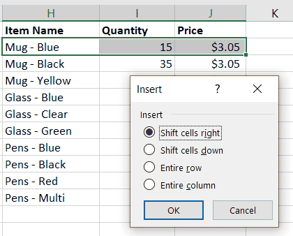
Excel GUI Prompt for How to Shift after Insert Cells
In most cases, you’ll probably be using xlShiftDown , which is the default for .Insert when referring to rows. However, sometimes you might want to copy to the right, say for a visual check after the subroutine runs:
This will produce the following result, where the range H2:J2 was inserted and the original values were moved to the right:
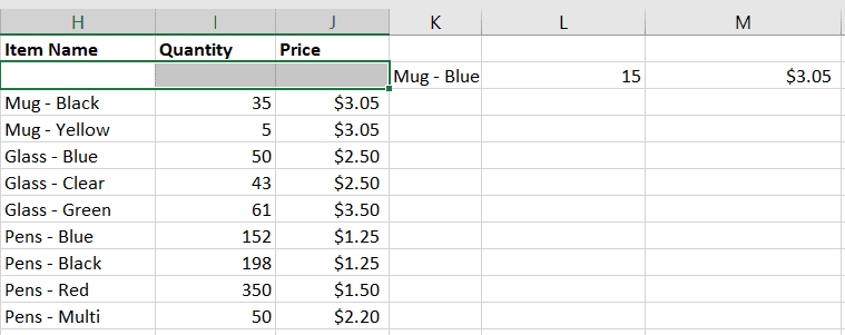
Cells Shifted to Right
The other optional parameter chooses where to copy the format of the inserted cells from. The default is xlFormatFromLeftOrAbove . In our table example, if we insert at «A2:E2» , we copy the cell formatting from «A1:E1» . Since this is our header, the inserted cells are initially set as bolded font. In order to ensure we have non-bold font, you should explicitly specify the CopyOrigin parameter:
This ensures that the inserted cells use the format of the cells below the range before the insertion instead of what’s above (the header format).
The Entire Row Property
The Excel GUI prompt above also allows you to insert an Entire Row . From our example earlier, this would affect the order table on the left and all other cells on the sheet, including the inventory table on the right. It’s equivalent to the Guessable Method, except the initial reference is a range of cells rather than the Rows collection directly.
To replicate the GUI’s Insert Entire Row from this example, you’ll add the the EntireRow property of the Range object:
This is most useful if you only have a cell location (especially a relative location, so you don’t know the true location) and you want to insert a full row.
Conclusion
Now you can insert rows across the entire sheet or only for specific ranges using VBA. In the latter case, you can now also choose whether to shift the cells down or to the right of the newly-inserted cells. And finally, you can choose the format of the new cells from the surrounding, existing cells.
You also learned a little about the EntireRow property, which can be useful in same instances, especially when programming complex macros where you don’t know the exact cell reference.
Ready to do more with VBA?
We put together a giant PDF with over 300 pre-built macros and we want you to have it for free. Enter your email address below and we’ll send you a copy along with our VBA Developer Kit, loaded with VBA tips, tricks and shortcuts.
Before we go, I want to let you know we designed a suite of VBA Cheat Sheets to make it easier for you to write better macros. We included over 200 tips and 140 macro examples so they have everything you need to know to become a better VBA programmer.
This article was written by Cory Sarver, a contributing writer for The VBA Tutorials Blog. Visit him on LinkedIn and his personal page.
Источник
| title | keywords | f1_keywords | ms.prod | api_name | ms.assetid | ms.date | ms.localizationpriority |
|---|---|---|---|---|---|---|---|
|
Range object (Excel) |
vbaxl10.chm143072 |
vbaxl10.chm143072 |
excel |
Excel.Range |
b8207778-0dcc-4570-1234-f130532cc8cd |
08/14/2019 |
high |
Range object (Excel)
Represents a cell, a row, a column, a selection of cells containing one or more contiguous blocks of cells, or a 3D range.
[!includeAdd-ins note]
Remarks
The default member of Range forwards calls without parameters to the Value property and calls with parameters to the Item member. Accordingly, someRange = someOtherRange is equivalent to someRange.Value = someOtherRange.Value, someRange(1) to someRange.Item(1) and someRange(1,1) to someRange.Item(1,1).
The following properties and methods for returning a Range object are described in the Example section:
- Range and Cells properties of the Worksheet object
- Range and Cells properties of the Range object
- Rows and Columns properties of the Worksheet object
- Rows and Columns properties of the Range object
- Offset property of the Range object
- Union method of the Application object
Example
Use Range (arg), where arg names the range, to return a Range object that represents a single cell or a range of cells. The following example places the value of cell A1 in cell A5.
Worksheets("Sheet1").Range("A5").Value = _
    Worksheets("Sheet1").Range("A1").Value
The following example fills the range A1:H8 with random numbers by setting the formula for each cell in the range. When it’s used without an object qualifier (an object to the left of the period), the Range property returns a range on the active sheet. If the active sheet isn’t a worksheet, the method fails.
Use the Activate method of the Worksheet object to activate a worksheet before you use the Range property without an explicit object qualifier.
Worksheets("Sheet1").Activate
Range("A1:H8").Formula = "=Rand()"    'Range is on the active sheet
The following example clears the contents of the range named Criteria.
[!NOTE]
If you use a text argument for the range address, you must specify the address in A1-style notation (you cannot use R1C1-style notation).
Worksheets(1).Range("Criteria").ClearContents
Use Cells on a worksheet to obtain a range consisting all single cells on the worksheet. You can access single cells via Item(row, column), where row is the row index and column is the column index.
Item can be omitted since the call is forwarded to it by the default member of Range.
The following example sets the value of cell A1 to 24 and of cell B1 to 42 on the first sheet of the active workbook.
Worksheets(1).Cells(1, 1).Value = 24
Worksheets(1).Cells.Item(1, 2).Value = 42
The following example sets the formula for cell A2.
ActiveSheet.Cells(2, 1).Formula = "=Sum(B1:B5)"
Although you can also use Range("A1") to return cell A1, there may be times when the Cells property is more convenient because you can use a variable for the row or column. The following example creates column and row headings on Sheet1. Be aware that after the worksheet has been activated, the Cells property can be used without an explicit sheet declaration (it returns a cell on the active sheet).
[!NOTE]
Although you could use Visual Basic string functions to alter A1-style references, it is easier (and better programming practice) to use theCells(1, 1)notation.
Sub SetUpTable()
Worksheets("Sheet1").Activate
For TheYear = 1 To 5
    Cells(1, TheYear + 1).Value = 1990 + TheYear
Next TheYear
For TheQuarter = 1 To 4
    Cells(TheQuarter + 1, 1).Value = "Q" & TheQuarter
Next TheQuarter
End Sub
Use_expression_.Cells, where expression is an expression that returns a Range object, to obtain a range with the same address consisting of single cells.
On such a range, you access single cells via Item(row, column), where are relative to the upper-left corner of the first area of the range.
Item can be omitted since the call is forwarded to it by the default member of Range.
The following example sets the formula for cell C5 and D5 of the first sheet of the active workbook.
Worksheets(1).Range("C5:C10").Cells(1, 1).Formula = "=Rand()"
Worksheets(1).Range("C5:C10").Cells.Item(1, 2).Formula = "=Rand()"
Use Range (cell1, cell2), where cell1 and cell2 are Range objects that specify the start and end cells, to return a Range object. The following example sets the border line style for cells A1:J10.
[!NOTE]
Be aware that the period in front of each occurrence of the Cells property is required if the result of the preceding With statement is to be applied to the Cells property. In this case, it indicates that the cells are on worksheet one (without the period, the Cells property would return cells on the active sheet).
With Worksheets(1)
    .Range(.Cells(1, 1), _
        .Cells(10, 10)).Borders.LineStyle = xlThick
End With
Use Rows on a worksheet to obtain a range consisting all rows on the worksheet. You can access single rows via Item(row), where row is the row index.
Item can be omitted since the call is forwarded to it by the default member of Range.
[!NOTE]
It’s not legal to provide the second parameter of Item for ranges consisting of rows. You first have to convert it to single cells via Cells.
The following example deletes row 5 and 10 of the first sheet of the active workbook.
Worksheets(1).Rows(10).Delete
Worksheets(1).Rows.Item(5).Delete
Use Columns on a worksheet to obtain a range consisting all columns on the worksheet. You can access single columns via Item(row) [sic], where row is the column index given as a number or as an A1-style column address.
Item can be omitted since the call is forwarded to it by the default member of Range.
[!NOTE]
It’s not legal to provide the second parameter of Item for ranges consisting of columns. You first have to convert it to single cells via Cells.
The following example deletes column «B», «C», «E», and «J» of the first sheet of the active workbook.
Worksheets(1).Columns(10).Delete
Worksheets(1).Columns.Item(5).Delete
Worksheets(1).Columns("C").Delete
Worksheets(1).Columns.Item("B").Delete
Use_expression_.Rows, where expression is an expression that returns a Range object, to obtain a range consisting of the rows in the first area of the range.
You can access single rows via Item(row), where row is the relative row index from the top of the first area of the range.
Item can be omitted since the call is forwarded to it by the default member of Range.
[!NOTE]
It’s not legal to provide the second parameter of Item for ranges consisting of rows. You first have to convert it to single cells via Cells.
The following example deletes the ranges C8:D8 and C6:D6 of the first sheet of the active workbook.
Worksheets(1).Range("C5:D10").Rows(4).Delete
Worksheets(1).Range("C5:D10").Rows.Item(2).Delete
Use_expression_.Columns, where expression is an expression that returns a Range object, to obtain a range consisting of the columns in the first area of the range.
You can access single columns via Item(row) [sic], where row is the relative column index from the left of the first area of the range given as a number or as an A1-style column address.
Item can be omitted since the call is forwarded to it by the default member of Range.
[!NOTE]
It’s not legal to provide the second parameter of Item for ranges consisting of columns. You first have to convert it to single cells via Cells.
The following example deletes the ranges L2:L10, G2:G10, F2:F10 and D2:D10 of the first sheet of the active workbook.
Worksheets(1).Range("C5:Z10").Columns(10).Delete
Worksheets(1).Range("C5:Z10").Columns.Item(5).Delete
Worksheets(1).Range("C5:Z10").Columns("D").Delete
Worksheets(1).Range("C5:Z10").Columns.Item("B").Delete
Use Offset (row, column), where row and column are the row and column offsets, to return a range at a specified offset to another range. The following example selects the cell three rows down from and one column to the right of the cell in the upper-left corner of the current selection. You cannot select a cell that is not on the active sheet, so you must first activate the worksheet.
Worksheets("Sheet1").Activate
  'Can't select unless the sheet is active
Selection.Offset(3, 1).Range("A1").Select
Use Union (range1, range2, …) to return multiple-area ranges—that is, ranges composed of two or more contiguous blocks of cells. The following example creates an object defined as the union of ranges A1:B2 and C3:D4, and then selects the defined range.
Dim r1 As Range, r2 As Range, myMultiAreaRange As Range
Worksheets("sheet1").Activate
Set r1 = Range("A1:B2")
Set r2 = Range("C3:D4")
Set myMultiAreaRange = Union(r1, r2)
myMultiAreaRange.Select
If you work with selections that contain more than one area, the Areas property is useful. It divides a multiple-area selection into individual Range objects and then returns the objects as a collection. Use the Count property on the returned collection to verify a selection that contains more than one area, as shown in the following example.
Sub NoMultiAreaSelection()
    NumberOfSelectedAreas = Selection.Areas.Count
    If NumberOfSelectedAreas > 1 Then
        MsgBox "You cannot carry out this command " & _
            "on multi-area selections"
    End If
End Sub
This example uses the AdvancedFilter method of the Range object to create a list of the unique values, and the number of times those unique values occur, in the range of column A.
Sub Create_Unique_List_Count()
    'Excel workbook, the source and target worksheets, and the source and target ranges.
    Dim wbBook As Workbook
    Dim wsSource As Worksheet
    Dim wsTarget As Worksheet
    Dim rnSource As Range
    Dim rnTarget As Range
    Dim rnUnique As Range
    'Variant to hold the unique data
    Dim vaUnique As Variant
    'Number of unique values in the data
    Dim lnCount As Long

    'Initialize the Excel objects
    Set wbBook = ThisWorkbook
    With wbBook
        Set wsSource = .Worksheets("Sheet1")
        Set wsTarget = .Worksheets("Sheet2")
    End With

    'On the source worksheet, set the range to the data stored in column A
    With wsSource
        Set rnSource = .Range(.Range("A1"), .Range("A100").End(xlDown))
    End With

    'On the target worksheet, set the range as column A.
    Set rnTarget = wsTarget.Range("A1")

    'Use AdvancedFilter to copy the data from the source to the target,
    'while filtering for duplicate values.
    rnSource.AdvancedFilter Action:=xlFilterCopy, _
                            CopyToRange:=rnTarget, _
                            Unique:=True

    'On the target worksheet, set the unique range on Column A, excluding the first cell
    '(which will contain the "List" header for the column).
    With wsTarget
        Set rnUnique = .Range(.Range("A2"), .Range("A100").End(xlUp))
    End With

    'Assign all the values of the Unique range into the Unique variant.
    vaUnique = rnUnique.Value

    'Count the number of occurrences of every unique value in the source data,
    'and list it next to its relevant value.
    For lnCount = 1 To UBound(vaUnique)
        rnUnique(lnCount, 1).Offset(0, 1).Value = _
            Application.Evaluate("COUNTIF(" & _
            rnSource.Address(External:=True) & _
            ",""" & rnUnique(lnCount, 1).Text & """)")
    Next lnCount

    'Label the column of occurrences with "Occurrences"
    With rnTarget.Offset(0, 1)
        .Value = "Occurrences"
        .Font.Bold = True
    End With

End Sub
Methods
- Activate
- AddComment
- AddCommentThreaded
- AdvancedFilter
- AllocateChanges
- ApplyNames
- ApplyOutlineStyles
- AutoComplete
- AutoFill
- AutoFilter
- AutoFit
- AutoOutline
- BorderAround
- Calculate
- CalculateRowMajorOrder
- CheckSpelling
- Clear
- ClearComments
- ClearContents
- ClearFormats
- ClearHyperlinks
- ClearNotes
- ClearOutline
- ColumnDifferences
- Consolidate
- ConvertToLinkedDataType
- Copy
- CopyFromRecordset
- CopyPicture
- CreateNames
- Cut
- DataTypeToText
- DataSeries
- Delete
- DialogBox
- Dirty
- DiscardChanges
- EditionOptions
- ExportAsFixedFormat
- FillDown
- FillLeft
- FillRight
- FillUp
- Find
- FindNext
- FindPrevious
- FlashFill
- FunctionWizard
- Group
- Insert
- InsertIndent
- Justify
- ListNames
- Merge
- NavigateArrow
- NoteText
- Parse
- PasteSpecial
- PrintOut
- PrintPreview
- RemoveDuplicates
- RemoveSubtotal
- Replace
- RowDifferences
- Run
- Select
- SetCellDataTypeFromCell
- SetPhonetic
- Show
- ShowCard
- ShowDependents
- ShowErrors
- ShowPrecedents
- Sort
- SortSpecial
- Speak
- SpecialCells
- SubscribeTo
- Subtotal
- Table
- TextToColumns
- Ungroup
- UnMerge
Properties
- AddIndent
- Address
- AddressLocal
- AllowEdit
- Application
- Areas
- Borders
- Cells
- Characters
- Column
- Columns
- ColumnWidth
- Comment
- CommentThreaded
- Count
- CountLarge
- Creator
- CurrentArray
- CurrentRegion
- Dependents
- DirectDependents
- DirectPrecedents
- DisplayFormat
- End
- EntireColumn
- EntireRow
- Errors
- Font
- FormatConditions
- Formula
- FormulaArray
- FormulaHidden
- FormulaLocal
- FormulaR1C1
- FormulaR1C1Local
- HasArray
- HasFormula
- HasRichDataType
- Height
- Hidden
- HorizontalAlignment
- Hyperlinks
- ID
- IndentLevel
- Interior
- Item
- Left
- LinkedDataTypeState
- ListHeaderRows
- ListObject
- LocationInTable
- Locked
- MDX
- MergeArea
- MergeCells
- Name
- Next
- NumberFormat
- NumberFormatLocal
- Offset
- Orientation
- OutlineLevel
- PageBreak
- Parent
- Phonetic
- Phonetics
- PivotCell
- PivotField
- PivotItem
- PivotTable
- Precedents
- PrefixCharacter
- Previous
- QueryTable
- Range
- ReadingOrder
- Resize
- Row
- RowHeight
- Rows
- ServerActions
- ShowDetail
- ShrinkToFit
- SoundNote
- SparklineGroups
- Style
- Summary
- Text
- Top
- UseStandardHeight
- UseStandardWidth
- Validation
- Value
- Value2
- VerticalAlignment
- Width
- Worksheet
- WrapText
- XPath
See also
- Excel Object Model Reference
[!includeSupport and feedback]
“It is a capital mistake to theorize before one has data”- Sir Arthur Conan Doyle
This post covers everything you need to know about using Cells and Ranges in VBA. You can read it from start to finish as it is laid out in a logical order. If you prefer you can use the table of contents below to go to a section of your choice.
Topics covered include Offset property, reading values between cells, reading values to arrays and formatting cells.
A Quick Guide to Ranges and Cells
| Function | Takes | Returns | Example | Gives |
|---|---|---|---|---|
|
Range |
cell address | multiple cells | .Range(«A1:A4») | $A$1:$A$4 |
| Cells | row, column | one cell | .Cells(1,5) | $E$1 |
| Offset | row, column | multiple cells | Range(«A1:A2») .Offset(1,2) |
$C$2:$C$3 |
| Rows | row(s) | one or more rows | .Rows(4) .Rows(«2:4») |
$4:$4 $2:$4 |
| Columns | column(s) | one or more columns | .Columns(4) .Columns(«B:D») |
$D:$D $B:$D |
Download the Code
The Webinar
If you are a member of the VBA Vault, then click on the image below to access the webinar and the associated source code.
(Note: Website members have access to the full webinar archive.)

Introduction
This is the third post dealing with the three main elements of VBA. These three elements are the Workbooks, Worksheets and Ranges/Cells. Cells are by far the most important part of Excel. Almost everything you do in Excel starts and ends with Cells.
Generally speaking, you do three main things with Cells
- Read from a cell.
- Write to a cell.
- Change the format of a cell.
Excel has a number of methods for accessing cells such as Range, Cells and Offset.These can cause confusion as they do similar things and can lead to confusion
In this post I will tackle each one, explain why you need it and when you should use it.
Let’s start with the simplest method of accessing cells – using the Range property of the worksheet.
Important Notes
I have recently updated this article so that is uses Value2.
You may be wondering what is the difference between Value, Value2 and the default:
' Value2
Range("A1").Value2 = 56

' Value
Range("A1").Value = 56

' Default uses value
Range("A1") = 56
Using Value may truncate number if the cell is formatted as currency. If you don’t use any property then the default is Value.
It is better to use Value2 as it will always return the actual cell value(see this article from Charle Williams.)
The Range Property
The worksheet has a Range property which you can use to access cells in VBA. The Range property takes the same argument that most Excel Worksheet functions take e.g. “A1”, “A3:C6” etc.
The following example shows you how to place a value in a cell using the Range property.
' https://excelmacromastery.com/
Public Sub WriteToCell()

    ' Write number to cell A1 in sheet1 of this workbook
    ThisWorkbook.Worksheets("Sheet1").Range("A1").Value2 = 67

    ' Write text to cell A2 in sheet1 of this workbook
    ThisWorkbook.Worksheets("Sheet1").Range("A2").Value2 = "John Smith"

    ' Write date to cell A3 in sheet1 of this workbook
    ThisWorkbook.Worksheets("Sheet1").Range("A3").Value2 = #11/21/2017#

End Sub
As you can see Range is a member of the worksheet which in turn is a member of the Workbook. This follows the same hierarchy as in Excel so should be easy to understand. To do something with Range you must first specify the workbook and worksheet it belongs to.
For the rest of this post I will use the code name to reference the worksheet.

The following code shows the above example using the code name of the worksheet i.e. Sheet1 instead of ThisWorkbook.Worksheets(“Sheet1”).
' https://excelmacromastery.com/
Public Sub UsingCodeName()

    ' Write number to cell A1 in sheet1 of this workbook
    Sheet1.Range("A1").Value2 = 67

    ' Write text to cell A2 in sheet1 of this workbook
    Sheet1.Range("A2").Value2 = "John Smith"

    ' Write date to cell A3 in sheet1 of this workbook
    Sheet1.Range("A3").Value2 = #11/21/2017#

End Sub
You can also write to multiple cells using the Range property
' https://excelmacromastery.com/
Public Sub WriteToMulti()

    ' Write number to a range of cells
    Sheet1.Range("A1:A10").Value2 = 67

    ' Write text to multiple ranges of cells
    Sheet1.Range("B2:B5,B7:B9").Value2 = "John Smith"

End Sub
You can download working examples of all the code from this post from the top of this article.
The Cells Property of the Worksheet
The worksheet object has another property called Cells which is very similar to range. There are two differences
- Cells returns a range of one cell only.
- Cells takes row and column as arguments.
The example below shows you how to write values to cells using both the Range and Cells property
' https://excelmacromastery.com/
Public Sub UsingCells()

    ' Write to A1
    Sheet1.Range("A1").Value2 = 10
    Sheet1.Cells(1, 1).Value2  = 10

    ' Write to A10
    Sheet1.Range("A10").Value2 = 10
    Sheet1.Cells(10, 1).Value2  = 10

    ' Write to E1
    Sheet1.Range("E1").Value2 = 10
    Sheet1.Cells(1, 5).Value2  = 10

End Sub
You may be wondering when you should use Cells and when you should use Range. Using Range is useful for accessing the same cells each time the Macro runs.
For example, if you were using a Macro to calculate a total and write it to cell A10 every time then Range would be suitable for this task.
Using the Cells property is useful if you are accessing a cell based on a number that may vary. It is easier to explain this with an example.
In the following code, we ask the user to specify the column number. Using Cells gives us the flexibility to use a variable number for the column.
' https://excelmacromastery.com/
Public Sub WriteToColumn()

    Dim UserCol As Integer

    ' Get the column number from the user
    UserCol = Application.InputBox(" Please enter the column...", Type:=1)

    ' Write text to user selected column
    Sheet1.Cells(1, UserCol).Value2 = "John Smith"

End Sub
In the above example, we are using a number for the column rather than a letter.
To use Range here would require us to convert these values to the letter/number cell reference e.g. “C1”. Using the Cells property allows us to provide a row and a column number to access a cell.
Sometimes you may want to return more than one cell using row and column numbers. The next section shows you how to do this.
Using Cells and Range together
As you have seen you can only access one cell using the Cells property. If you want to return a range of cells then you can use Cells with Ranges as follows
' https://excelmacromastery.com/
Public Sub UsingCellsWithRange()

    With Sheet1
        ' Write 5 to Range A1:A10 using Cells property
        .Range(.Cells(1, 1), .Cells(10, 1)).Value2 = 5

        ' Format Range B1:Z1 to be bold
        .Range(.Cells(1, 2), .Cells(1, 26)).Font.Bold = True

    End With

End Sub
As you can see, you provide the start and end cell of the Range. Sometimes it can be tricky to see which range you are dealing with when the value are all numbers. Range has a property called Address which displays the letter/ number cell reference of any range. This can come in very handy when you are debugging or writing code for the first time.
In the following example we print out the address of the ranges we are using:
' https://excelmacromastery.com/
Public Sub ShowRangeAddress()

    ' Note: Using underscore allows you to split up lines of code
    With Sheet1

        ' Write 5 to Range A1:A10 using Cells property
        .Range(.Cells(1, 1), .Cells(10, 1)).Value2 = 5
        Debug.Print "First address is : " _
            + .Range(.Cells(1, 1), .Cells(10, 1)).Address

        ' Format Range B1:Z1 to be bold
        .Range(.Cells(1, 2), .Cells(1, 26)).Font.Bold = True
        Debug.Print "Second address is : " _
            + .Range(.Cells(1, 2), .Cells(1, 26)).Address

    End With

End Sub
In the example I used Debug.Print to print to the Immediate Window. To view this window select View->Immediate Window(or Ctrl G)


You can download all the code for this post from the top of this article.
The Offset Property of Range
Range has a property called Offset. The term Offset refers to a count from the original position. It is used a lot in certain areas of programming. With the Offset property you can get a Range of cells the same size and a certain distance from the current range. The reason this is useful is that sometimes you may want to select a Range based on a certain condition. For example in the screenshot below there is a column for each day of the week. Given the day number(i.e. Monday=1, Tuesday=2 etc.) we need to write the value to the correct column.

We will first attempt to do this without using Offset.
' https://excelmacromastery.com/
' This sub tests with different values
Public Sub TestSelect()

    ' Monday
    SetValueSelect 1, 111.21
    ' Wednesday
    SetValueSelect 3, 456.99
    ' Friday
    SetValueSelect 5, 432.25
    ' Sunday
    SetValueSelect 7, 710.17

End Sub

' Writes the value to a column based on the day
Public Sub SetValueSelect(lDay As Long, lValue As Currency)

    Select Case lDay
        Case 1: Sheet1.Range("H3").Value2 = lValue
        Case 2: Sheet1.Range("I3").Value2 = lValue
        Case 3: Sheet1.Range("J3").Value2 = lValue
        Case 4: Sheet1.Range("K3").Value2 = lValue
        Case 5: Sheet1.Range("L3").Value2 = lValue
        Case 6: Sheet1.Range("M3").Value2 = lValue
        Case 7: Sheet1.Range("N3").Value2 = lValue
    End Select

End Sub
As you can see in the example, we need to add a line for each possible option. This is not an ideal situation. Using the Offset Property provides a much cleaner solution
' https://excelmacromastery.com/
' This sub tests with different values
Public Sub TestOffset()

    DayOffSet 1, 111.01
    DayOffSet 3, 456.99
    DayOffSet 5, 432.25
    DayOffSet 7, 710.17

End Sub

Public Sub DayOffSet(lDay As Long, lValue As Currency)

    ' We use the day value with offset specify the correct column
    Sheet1.Range("G3").Offset(, lDay).Value2 = lValue

End Sub
As you can see this solution is much better. If the number of days in increased then we do not need to add any more code. For Offset to be useful there needs to be some kind of relationship between the positions of the cells. If the Day columns in the above example were random then we could not use Offset. We would have to use the first solution.
One thing to keep in mind is that Offset retains the size of the range. So .Range(“A1:A3”).Offset(1,1) returns the range B2:B4. Below are some more examples of using Offset
' https://excelmacromastery.com/
Public Sub UsingOffset()

    ' Write to B2 - no offset
    Sheet1.Range("B2").Offset().Value2 = "Cell B2"

    ' Write to C2 - 1 column to the right
    Sheet1.Range("B2").Offset(, 1).Value2 = "Cell C2"

    ' Write to B3 - 1 row down
    Sheet1.Range("B2").Offset(1).Value2 = "Cell B3"

    ' Write to C3 - 1 column right and 1 row down
    Sheet1.Range("B2").Offset(1, 1).Value2 = "Cell C3"

    ' Write to A1 - 1 column left and 1 row up
    Sheet1.Range("B2").Offset(-1, -1).Value2 = "Cell A1"

    ' Write to range E3:G13 - 1 column right and 1 row down
    Sheet1.Range("D2:F12").Offset(1, 1).Value2 = "Cells E3:G13"

End Sub
Using the Range CurrentRegion
CurrentRegion returns a range of all the adjacent cells to the given range.
In the screenshot below you can see the two current regions. I have added borders to make the current regions clear.

A row or column of blank cells signifies the end of a current region.
You can manually check the CurrentRegion in Excel by selecting a range and pressing Ctrl + Shift + *.
If we take any range of cells within the border and apply CurrentRegion, we will get back the range of cells in the entire area.
For example
Range(“B3”).CurrentRegion will return the range B3:D14
Range(“D14”).CurrentRegion will return the range B3:D14
Range(“C8:C9”).CurrentRegion will return the range B3:D14
and so on
How to Use
We get the CurrentRegion as follows
' Current region will return B3:D14 from above example
Dim rg As Range
Set rg = Sheet1.Range("B3").CurrentRegion
Read Data Rows Only
Read through the range from the second row i.e.skipping the header row
' Current region will return B3:D14 from above example
Dim rg As Range
Set rg = Sheet1.Range("B3").CurrentRegion

' Start at row 2 - row after header
Dim i As Long
For i = 2 To rg.Rows.Count
    ' current row, column 1 of range
    Debug.Print rg.Cells(i, 1).Value2
Next i
Remove Header
Remove header row(i.e. first row) from the range. For example if range is A1:D4 this will return A2:D4
' Current region will return B3:D14 from above example
Dim rg As Range
Set rg = Sheet1.Range("B3").CurrentRegion

' Remove Header
Set rg = rg.Resize(rg.Rows.Count - 1).Offset(1)

' Start at row 1 as no header row
Dim i As Long
For i = 1 To rg.Rows.Count
    ' current row, column 1 of range
    Debug.Print rg.Cells(i, 1).Value2
Next i
Using Rows and Columns as Ranges
If you want to do something with an entire Row or Column you can use the Rows or Columns property of the Worksheet. They both take one parameter which is the row or column number you wish to access
' https://excelmacromastery.com/
Public Sub UseRowAndColumns()

    ' Set the font size of column B to 9
    Sheet1.Columns(2).Font.Size = 9

    ' Set the width of columns D to F
    Sheet1.Columns("D:F").ColumnWidth = 4

    ' Set the font size of row 5 to 18
    Sheet1.Rows(5).Font.Size = 18

End Sub
Using Range in place of Worksheet
You can also use Cells, Rows and Columns as part of a Range rather than part of a Worksheet. You may have a specific need to do this but otherwise I would avoid the practice. It makes the code more complex. Simple code is your friend. It reduces the possibility of errors.
The code below will set the second column of the range to bold. As the range has only two rows the entire column is considered B1:B2
' https://excelmacromastery.com/
Public Sub UseColumnsInRange()

    ' This will set B1 and B2 to be bold
    Sheet1.Range("A1:C2").Columns(2).Font.Bold = True

End Sub
You can download all the code for this post from the top of this article.
Reading Values from one Cell to another
In most of the examples so far we have written values to a cell. We do this by placing the range on the left of the equals sign and the value to place in the cell on the right. To write data from one cell to another we do the same. The destination range goes on the left and the source range goes on the right.
The following example shows you how to do this:
' https://excelmacromastery.com/
Public Sub ReadValues()

    ' Place value from B1 in A1
    Sheet1.Range("A1").Value2 = Sheet1.Range("B1").Value2

    ' Place value from B3 in sheet2 to cell A1
    Sheet1.Range("A1").Value2 = Sheet2.Range("B3").Value2

    ' Place value from B1 in cells A1 to A5
    Sheet1.Range("A1:A5").Value2 = Sheet1.Range("B1").Value2

    ' You need to use the "Value" property to read multiple cells
    Sheet1.Range("A1:A5").Value2 = Sheet1.Range("B1:B5").Value2

End Sub
As you can see from this example it is not possible to read from multiple cells. If you want to do this you can use the Copy function of Range with the Destination parameter
' https://excelmacromastery.com/
Public Sub CopyValues()

    ' Store the copy range in a variable
    Dim rgCopy As Range
    Set rgCopy = Sheet1.Range("B1:B5")

    ' Use this to copy from more than one cell
    rgCopy.Copy Destination:=Sheet1.Range("A1:A5")

    ' You can paste to multiple destinations
    rgCopy.Copy Destination:=Sheet1.Range("A1:A5,C2:C6")

End Sub
The Copy function copies everything including the format of the cells. It is the same result as manually copying and pasting a selection. You can see more about it in the Copying and Pasting Cells section.
Using the Range.Resize Method
When copying from one range to another using assignment(i.e. the equals sign), the destination range must be the same size as the source range.
Using the Resize function allows us to resize a range to a given number of rows and columns.
For example:
' https://excelmacromastery.com/
Sub ResizeExamples()

    ' Prints A1
    Debug.Print Sheet1.Range("A1").Address

    ' Prints A1:A2
    Debug.Print Sheet1.Range("A1").Resize(2, 1).Address

    ' Prints A1:A5
    Debug.Print Sheet1.Range("A1").Resize(5, 1).Address

    ' Prints A1:D1
    Debug.Print Sheet1.Range("A1").Resize(1, 4).Address

    ' Prints A1:C3
    Debug.Print Sheet1.Range("A1").Resize(3, 3).Address

End Sub
When we want to resize our destination range we can simply use the source range size.
In other words, we use the row and column count of the source range as the parameters for resizing:
' https://excelmacromastery.com/
Sub Resize()

    Dim rgSrc As Range, rgDest As Range

    ' Get all the data in the current region
    Set rgSrc = Sheet1.Range("A1").CurrentRegion

      ' Get the range destination
    Set rgDest = Sheet2.Range("A1")
    Set rgDest = rgDest.Resize(rgSrc.Rows.Count, rgSrc.Columns.Count)

    rgDest.Value2 = rgSrc.Value2

End Sub
We can do the resize in one line if we prefer:
' https://excelmacromastery.com/
Sub ResizeOneLine()

    Dim rgSrc As Range

    ' Get all the data in the current region
    Set rgSrc = Sheet1.Range("A1").CurrentRegion

    With rgSrc
        Sheet2.Range("A1").Resize(.Rows.Count, .Columns.Count).Value2 = .Value2
    End With

End Sub
Reading Values to variables
We looked at how to read from one cell to another. You can also read from a cell to a variable. A variable is used to store values while a Macro is running. You normally do this when you want to manipulate the data before writing it somewhere. The following is a simple example using a variable. As you can see the value of the item to the right of the equals is written to the item to the left of the equals.
' https://excelmacromastery.com/
Public Sub UseVariables()

    ' Create
    Dim number As Long

    ' Read number from cell
    number = Sheet1.Range("A1").Value2

    ' Add 1 to value
    number = number + 1

    ' Write new value to cell
    Sheet1.Range("A2").Value2 = number

End Sub
To read text to a variable you use a variable of type String:
' https://excelmacromastery.com/
Public Sub UseVariableText()

    ' Declare a variable of type string
    Dim text As String

    ' Read value from cell
    text = Sheet1.Range("A1").Value2

    ' Write value to cell
    Sheet1.Range("A2").Value2 = text

End Sub
You can write a variable to a range of cells. You just specify the range on the left and the value will be written to all cells in the range.
' https://excelmacromastery.com/
Public Sub VarToMulti()

    ' Read value from cell
    Sheet1.Range("A1:B10").Value2 = 66

End Sub
You cannot read from multiple cells to a variable. However you can read to an array which is a collection of variables. We will look at doing this in the next section.
How to Copy and Paste Cells
If you want to copy and paste a range of cells then you do not need to select them. This is a common error made by new VBA users.
Note: We normally use Range.Copy when we want to copy formats, formulas, validation. If we want to copy values it is not the most efficient method.
I have written a complete guide to copying data in Excel VBA here.
You can simply copy a range of cells like this:
Range("A1:B4").Copy Destination:=Range("C5")
Using this method copies everything – values, formats, formulas and so on. If you want to copy individual items you can use the PasteSpecial property of range.
It works like this
Range("A1:B4").Copy
Range("F3").PasteSpecial Paste:=xlPasteValues
Range("F3").PasteSpecial Paste:=xlPasteFormats
Range("F3").PasteSpecial Paste:=xlPasteFormulas
The following table shows a full list of all the paste types
| Paste Type |
|---|
| xlPasteAll |
| xlPasteAllExceptBorders |
| xlPasteAllMergingConditionalFormats |
| xlPasteAllUsingSourceTheme |
| xlPasteColumnWidths |
| xlPasteComments |
| xlPasteFormats |
| xlPasteFormulas |
| xlPasteFormulasAndNumberFormats |
| xlPasteValidation |
| xlPasteValues |
| xlPasteValuesAndNumberFormats |
Reading a Range of Cells to an Array
You can also copy values by assigning the value of one range to another.
Range("A3:Z3").Value2 = Range("A1:Z1").Value2
The value of range in this example is considered to be a variant array. What this means is that you can easily read from a range of cells to an array. You can also write from an array to a range of cells. If you are not familiar with arrays you can check them out in this post.
The following code shows an example of using an array with a range:
' https://excelmacromastery.com/
Public Sub ReadToArray()

    ' Create dynamic array
    Dim StudentMarks() As Variant

    ' Read 26 values into array from the first row
    StudentMarks = Range("A1:Z1").Value2

    ' Do something with array here

    ' Write the 26 values to the third row
    Range("A3:Z3").Value2 = StudentMarks

End Sub
Keep in mind that the array created by the read is a 2 dimensional array. This is because a spreadsheet stores values in two dimensions i.e. rows and columns
Going through all the cells in a Range
Sometimes you may want to go through each cell one at a time to check value.
You can do this using a For Each loop shown in the following code
' https://excelmacromastery.com/
Public Sub TraversingCells()

    ' Go through each cells in the range
    Dim rg As Range
    For Each rg In Sheet1.Range("A1:A10,A20")
        ' Print address of cells that are negative
        If rg.Value < 0 Then
            Debug.Print rg.Address + " is negative."
        End If
    Next

End Sub
You can also go through consecutive Cells using the Cells property and a standard For loop.
The standard loop is more flexible about the order you use but it is slower than a For Each loop.
' https://excelmacromastery.com/
Public Sub TraverseCells()

    ' Go through cells from A1 to A10
    Dim i As Long
    For i = 1 To 10
        ' Print address of cells that are negative
        If Range("A" & i).Value < 0 Then
            Debug.Print Range("A" & i).Address + " is negative."
        End If
    Next

    ' Go through cells in reverse i.e. from A10 to A1
    For i = 10 To 1 Step -1
        ' Print address of cells that are negative
        If Range("A" & i) < 0 Then
            Debug.Print Range("A" & i).Address + " is negative."
        End If
    Next

End Sub
Formatting Cells
Sometimes you will need to format the cells the in spreadsheet. This is actually very straightforward. The following example shows you various formatting you can add to any range of cells
' https://excelmacromastery.com/
Public Sub FormattingCells()

    With Sheet1

        ' Format the font
        .Range("A1").Font.Bold = True
        .Range("A1").Font.Underline = True
        .Range("A1").Font.Color = rgbNavy

        ' Set the number format to 2 decimal places
        .Range("B2").NumberFormat = "0.00"
        ' Set the number format to a date
        .Range("C2").NumberFormat = "dd/mm/yyyy"
        ' Set the number format to general
        .Range("C3").NumberFormat = "General"
        ' Set the number format to text
        .Range("C4").NumberFormat = "Text"

        ' Set the fill color of the cell
        .Range("B3").Interior.Color = rgbSandyBrown

        ' Format the borders
        .Range("B4").Borders.LineStyle = xlDash
        .Range("B4").Borders.Color = rgbBlueViolet

    End With

End Sub
Main Points
The following is a summary of the main points
- Range returns a range of cells
- Cells returns one cells only
- You can read from one cell to another
- You can read from a range of cells to another range of cells.
- You can read values from cells to variables and vice versa.
- You can read values from ranges to arrays and vice versa
- You can use a For Each or For loop to run through every cell in a range.
- The properties Rows and Columns allow you to access a range of cells of these types
What’s Next?
Free VBA Tutorial If you are new to VBA or you want to sharpen your existing VBA skills then why not try out the The Ultimate VBA Tutorial.
Related Training: Get full access to the Excel VBA training webinars and all the tutorials.
(NOTE: Planning to build or manage a VBA Application? Learn how to build 10 Excel VBA applications from scratch.)
Excel VBA Referencing Ranges — Range, Cells, Item, Rows & Columns Properties; Offset; ActiveCell; Selection; Insert
You can refer to or access a worksheet range using properties and methods of the Range object. A Range Object refers to a cell or a range of cells. It can be a row, a column or a selection of cells comprising of one or more rectangular / contiguous blocks of cells. One of the most important aspects in vba coding is referencing and using Ranges within a Worksheet. This section (divided into 2 parts) covers various properties and methods for referencing, accessing & using ranges, divided under the following chapters.
Excel VBA Referencing Ranges — Range, Cells, Item, Rows & Columns Properties; Offset; ActiveCell; Selection; Insert:
Range Property, Cells / Item / Rows / Columns Properties, Offset & Relative Referencing, Cell Address;
Activate & Select Cells; the ActiveCell & Selection;
Entire Row & Entire Column Properties, Inserting Cells/Rows/Columns using the Insert Method;
Excel VBA Refer to Ranges — Union & Intersect; Resize; Areas, CurrentRegion, UsedRange & End Properties; SpecialCells Method:
Ranges — Union & Intersect;
Resize a Range;
Referencing — Contiguous Block(s) of Cells, Range of Contiguous Data, Cells Meeting a Specified Criteria, Used Range, Cell at the End of a Block / Region, Last Used Row or Column;
Related Links:
Working with Objects in Excel VBA
Excel VBA Application Object, the Default Object in Excel
Excel VBA Workbook Object, working with Workbooks in Excel
Microsoft Excel VBA — Worksheets
Excel VBA Custom Classes and Objects
——————————————————————————————-
Contents:
Range Property, Cells / Item / Rows / Columns Properties, Offset & Relative Referencing, Cell Address
Activate & Select Cells; the ActiveCell & Selection
Entire Row & Entire Column Properties, Inserting Cells/Rows/Columns using the Insert Method
——————————————————————————————-
Range Property, Cells / Item / Rows / Columns Properties, Offset & Relative Referencing, Cell Address
A Range Object refers to a cell or a range of cells. It can be a row, a column or a selection of cells comprising of one or more rectangular / contiguous blocks of cells. A Range object is always with reference to a specific worksheet, and Excel currently does not support Range objects spread over multiple worksheets.
Range object refers to a single cell:
Dim rng As Range
Set rng = Range(«A1»)
Range object refers to a block of contiguous cells:
Dim rng As Range
Set rng = Range(«A1:C3»)
Range object refers to a row:
Dim rng As Range
Set rng = Rows(1)
Range object refers to multiple columns:
Dim rng As Range
Set rng = Columns(«A:C»)
Range object refers to 2 or more blocks of contiguous cells — using the ‘Union method’ & ‘Selection’ (these have been explained in detail later in this section).
Union method:
Dim rng1 As Range, rng2 As Range, rngUnion As Range
‘set a contiguous block of cells as the first range:
Set rng1 = Range(«A1:B2»)
‘set another contiguous block of cells as the second range:
Set rng2 = Range(«D3:E4»)
‘assign a variable (range object) to represent the union of the 2 ranges, using the Union method:
Set rngUnion = Union(rng1, rng2)
‘set interior color for the range which is the union of 2 range objects:
rngUnion.Interior.Color = vbYellow
Selection property:
‘select 2 contiguous block of cells, using the Select method:
Range(«A1:B2,D3:E4»).Select
‘perform action (set interior color of cells to yellow) on the Selection, which is a Range object:
Selection.Interior.Color = vbYellow
Range property of the Worksheet object ie. Worksheet.Range Property. Syntax: WorksheetObject.Range(Cell1, Cell2). You have an option to use only the Cell1 argument and in this case it will have to be a A1-style reference to a range which can include a range operator (colon) or the union operator (comma), or the reference to a range can be a defined name. Examples of using this type of reference are Worksheets(«Sheet1»).Range(«A1») which refers to cell A1; or Worksheets(«Sheet1»).Range(«A1:B3») which refers to the cells A1, A2, A3, B1, B2 & B3. When both the Cell1 & Cell2 arguments are used (cell1 and cell2 are Range objects), these refer to the cells at the top-left corner and the lower-right corner of the range (ie. the start and end cells of the range), and these arguments can be a single cell, an entire row or column or a single named cell. An example of using this type of reference is Worksheets(«Sheet1»).Range(Cells(1, 1), Cells(3, 2)) which refers to the cells A1, A2, A3, B1, B2 & B3. Omitting the object qualifier will default to the active sheet viz. using the code Range(«A1») will return cell A1 of the active sheet, and will be the same as using Application.Range(«A1») or ActiveSheet.Range(«A1»).
Range property of the Range object: Use the Range.Range property [Syntax: RangeObject.Range(Cell1,Cell2)] for relative referencing ie. to access a range relative to a range object. For example, Worksheets(«Sheet1»).Range(«C5:E8»).Range(«A1») will refer to Range(«C5») and Worksheets(«Sheet1»).Range(«C5:E8»).Range(«B2») will refer to Range(«D6»).
Shortcut Range Reference: As compared to using the Range property, you can also use a shorter code to refer to a range by using square brackets to enclose an A1-style reference or a name. While using square brackets, you do not type the Range word or wrap the range in quotation marks to make it a string. Using square brackets is similar to applying the Evaluate method of the Application object. The Range property or the Evaluate method use a string argument which enables you to manipulate the string with vba code, whereas using the square brackets will be inflexible in this respect. Examples: using [A1].Value = 5 is equivalent to using Range(«A1»).Value = 5; using [A1:A3,B2:B4,C3:D5].Interior.Color = vbRed is equivalent to Range(«A1:A3,B2:B4,C3:D5»).Interior.Color = vbRed; and with named ranges, [Score].Interior.Color = vbBlue is equivalent to Range(«Score»).Interior.Color = vbBlue. Using square brackets only enables reference to fixed ranges which is a significant shortcoming. Using the Range property enables you to manipulate the string argument with vba code so that you can use variables to refer to a dynamic range, as illustrated below:
Sub DynamicRangeVariable()
‘using a variable to refer a dynamic range.
Dim i As Integer
‘enters the text «Hello» in each cell from B1 to B5:
For i = 1 To 5
Range(«B» & i) = «Hello»
Next
End Sub
The Cells Property returns a Range object referring to all cells in a worksheet or a range, as it can be used with respect to an Application object, a Worksheet object or a Range object. Application.Cells Property refers to all cells in the active worksheet. You can use the code Application.Cells or omit the object qualifier (this property is a member of ‘globals’) and use the code Cells to refer to all cells of the active worksheet. The Worksheet.Cells Property (Syntax: WorksheetObject.Cells) refers to all cells of a specified worksheet. Use the code Worksheets(«Sheet1»).Cells to refer to all cells of worksheet named «Sheet1». Use the Range.Cells Property ro refer to cells in a specified range — (Syntax: RangeObject.Cells). This property can be used as Range(«A1:B5»).Cells, however using the word cells in this case is immaterial because with or without this word the code will refer to the range A1:B5. To refer to a specific cell, use the Item property of the Range object (as explained in detail below) by specifying the relative row and column positions after the Cells keyword, viz. Worksheets(«Sheet1»).Cells.Item(2, 3) refers to range C2 and Worksheets(«Sheet1»).Range(«C2»).Cells(2, 3) will refer to range E3. Because the Item property is the Range object’s default property you can omit the Item word word and use the code Worksheets(«Sheet1»).Cells(2, 3) which also refers to range C2. You may find it preferable in some cases to use Worksheets(«Sheet1»).Cells(2, 3) over Worksheets(«Sheet1»).Range(«C2») because variables for the row and column can easily be used therein.
Item property of the Range object: Use the Range.Item Property to return a range as offset to the specified range. Syntax: RangeObject.Item(RowIndex, ColumnIndex). The Item word can be omitted because Item is the Range object’s default property. It is necessary to specify the RowIndex argument while ColumnIndex is optional. RowIndex is the index number of the cell, starting with 1 and increasing from left to right and then down. Worksheets(«Sheet1»).Cells.Item(1) or Worksheets(«Sheet1»).Cells(1) refers to range A1 (the top-left cell in the worksheet), Worksheets(«Sheet1»).Cells(2) refers to range B1 (cell next to the right of the top-left cell). While using a single-parameter reference of the Item property (ie. RowIndex), if index exceeds the number of columns in the specified range, the reference will wrap to successive rows within the range columns. Omitting the object qualifier will default to active sheet. Cells(16385) refers to range A2 of the active sheet in Excel 2007 which has 16384 columns, and Cells(16386) refers to range B2, and so on. Also note that RowIndex and ColumnIndex are offsets and relative to the specified Range (ie. relative to the top-left corner of the specified range). Both Range(«B3»).Item(1) and Range(«B3:D6»).Item(1) refer to range B3. The following refer to range D4, the sixth cell in the range: Range(«B3:D6»).Item(6) or Range(«B3:D6»).Cells(6) or Range(«B3:D6»)(6). ColumnIndex refers to the column number of the cell, can be a number starting with 1 or can be a string starting with the letter «A». Worksheets(«Sheet1»).Cells(2, 3) and Worksheets(«Sheet1»).Cells(2, «C») both refer to range C2 wherein the RowIndex is 2 and ColumnIndex is 3 (column C). Range(«C2»).Cells(2, 3) refers to range E3 in the active sheet, and Range(«C2»).Cells(4, 5) refers to range G5 in the active sheet. Using Range(«C2»).Item(2, 3) and Range(«C2»).Item(4, 5) has the same effect and will refer to range E3 & range G5 respectively. Using Range(«C2:D3»).Cells(2, 3) and Range(«C2:D3»).Cells(4, 5) will also refer to range E3 & range G5 respectively. Omitting the Item or Cells word — Range(«C2:D3»)(2, 3) and Range(«C2:D3»)(4, 5) also refers to range E3 & range G5 respectively. It is apparant here that you can refer to and return cells outside the original specified range, using the Item property.
Columns property of the Worksheet object: Use the Worksheet.Columns Property (Syntax: WorksheetObject.Columns) to refer to all columns in a worksheet which are returned as a Range object. Example: Worksheets(«Sheet1»).Columns will return all columns of the worksheet; Worksheets(«Sheet1»).Columns(1) returns the first column (column A) in the worksheet; Worksheets(«Sheet1»).Columns(«A») returns the first column (column A); Worksheets(«Sheet1»).Columns(«A:C») returns the columns A, B & C; and so on. Omitting the object qualifier will default to the active sheet viz. using the code Columns(1) will return the first column of the active sheet, and will be the same as using Application.Columns(1).
Columns property of the Range object: Use the Range.Columns Property (Syntax: RangeObject.Columns) to refer to columns in a specified range. Example1: color cells from all columns of the specified range ie. B2 to D4: Worksheets(«Sheet1»).Range(«B2:D4»).Columns.Interior.Color = vbYellow. Example2: color cells from first column of the range only ie. B2 to B4: Worksheets(«Sheet1»).Range(«B2:D4»).Columns(1).Interior.Color = vbGreen. If the specified range object contains multiple areas, the columns from the first area only will be returned by this property (Areas property has been explained in detail later in this section). Take the example of 2 areas in the specified range, first area being «B2:D4» and the second area being «F3:G6» — the following code will color cells from first column of the first area only ie. cells B2 to B4: Worksheets(«Sheet1»).Range(«B2:D4, F3:G6»).Columns(1).Interior.Color = vbRed. Omitting the object qualifier will default to active sheet — following will apply color to column A of the ActiveSheet: Columns(1).Interior.Color = vbRed.
Use the Worksheet.Rows Property (Syntax: WorksheetObject.Rows) to refer to all rows in a worksheet which are returned as a Range object. Example: Worksheets(«Sheet1»).Rows will return all rows of the worksheet; Worksheets(«Sheet1»).Rows(1) returns the first row (row one) in the worksheet; Worksheets(«Sheet1»).Rows(3) returns the third row (row three) in the worksheet; Worksheets(«Sheet1»).Rows(«1:3») returns the first 3 rows; and so on. Omitting the object qualifier will default to the active sheet viz. using the code Rows(1) will return the first row of the active sheet, and will be the same as using Application.Rows(1).
Use the Range.Rows Property (Syntax: RangeObject.Rows) to refer to rows in a specified range. Example1: color cells from all rows of the specified range ie. B2 to D4: Worksheets(«Sheet1»).Range(«B2:D4»).Rows.Interior.Color = vbYellow. Example2: color cells from first row of the range only ie. B2 to D2: Worksheets(«Sheet1»).Range(«B2:D4»).Rows(1).Interior.Color = vbGreen. If the specified range object contains multiple areas, the rows from the first area only will be returned by this property (Areas property has been explained in detail later in this section). Take the example of 2 areas in the specified range, first area being «B2:D4» and the second area being «F3:G6» — the following code will color cells from first row of the first area only ie. cells B2 to D2: Worksheets(«Sheet1»).Range(«B2:D4, F3:G6»).Rows(1).Interior.Color = vbRed. Omitting the object qualifier will default to active sheet — following will apply color to row one of the ActiveSheet: Rows(1).Interior.Color = vbRed.
To refer to a range as offset from a specified range, use the Range.Offset Property. Syntax: RangeObject.Offset(RowOffset, ColumnOffset). Both arguments are optional to specify. The RowOffset argument specifies the number of rows by which the specified range is offset — negative values indicating upward offset and positive values indicating downward offset, with default value being 0. The ColumnOffset argument specifies the number of columns by which the specified range is offset — negative values indicating left offset and positive values indicating right offset, with default value being 0. Examples: Range(«C5»).Offset(1, 2) offsets 1 row & 2 columns and refers to Range E6, Range(«C5:D7»).Offset(1, -2) offsets 1 row downward & 2 columns to the left and refers to Range (A6:B8).
Accessing a worksheet range, with vba code:-
Referencing a single cell:
Enter the value 10 in the cell A1 of the worksheet named «Sheet1» (omitting to mention a property with the Range object will assume the Value property, as shown below):
Worksheets(«Sheet1»).Range(«A1»).Value = 10
Worksheets(«Sheet1»).Range(«A1») = 10
Enter the value of 10 in range C2 of the active worksheet — using Cells(row, column) where row is the row index and column is the column index:
ActiveSheet.Cells(2, 3).Value = 10
Referencing a range of cells:
Enter the value 10 in the cells A1, A2, A3, B1, B2 & B3 (wherein the cells refer to the upper-left corner & lower-right corner of the range) of the active sheet:
ActiveSheet.Range(«A1:B3»).Value = 10
ActiveSheet.Range(«A1», «B3»).Value = 10
ActiveSheet.Range(Cells(1, 1), Cells(3, 2)) = 10
Enter the value 10 in the cells A1 & B3 of worksheet named «Sheet1»:
Worksheets(«Sheet1»).Range(«A1,B3»).Value = 10
Set the background color (red) for cells B2, B3, C2, C3, D2, D3 & H7 of worksheet named «Sheet3»:
ActiveWorkbook.Worksheets(«Sheet3»).
Range(«B2:D3,H7»).Interior.Color = vbRed
Enter the value 10 in the Named Range «Score» of the active worksheet, viz. you can name the Range(«B2:B3») as «Score» to insert 10 in the cells B2 & B3:
Range(«Score»).Value = 10
ActiveSheet.Range(«Score»).Value = 10
Select all the cells of the active worksheet:
ActiveSheet.Cells.Select
Cells.Select
Set the font to «Times New Roman» & the font size to 11, for all the cells of the active worksheet in the active workbook:
ActiveWorkbook.ActiveSheet.Cells.Font.Name = «Times New Roman»
ActiveSheet.Cells.Font.Size = 11
Cells.Font.Size = 11
Referencing Row(s) or Column(s):
Select all the Rows of active worksheet:
ActiveSheet.Rows.Select
Enter the value 10 in the Row number 2 (ie. every cell in second row), of worksheet named «Sheet1»:
Worksheets(«Sheet1»).Rows(2).Value = 10
Select all the Columns of the active worksheet:
ActiveSheet.Columns.Select
Columns.Select
Enter the value 10 in the Column number 3 (ie. every cell in column C), of the active worksheet:
ActiveSheet.Columns(3).Value = 10
Columns(«C»).Value = 10
Enter the value 10 in Column numbers 1, 2 & 3 (ie. every cell in columns A to C), of worksheet named «Sheet1»:
Worksheets(«Sheet1»).Columns(«A:C»).Value = 10
Relative Referencing:
Inserts the value 10 in Range C5 — reference starts from upper-left corner of the defined Range:
Range(«C5:E8»).Range(«A1») = 10
Inserts the value 10 in Range D6 — reference starts from upper-left corner of the defined Range:
Range(«C5:E8»).Range(«B2») = 10
Inserts the value 10 in Range E6 — offsets 1 row & 2 columns, using the Offset property:
Range(«C5»).Offset(1, 2) = 10
Inserts the value 10 in Range(«F7:H10») — offsets 2 rows & 3 columns, using the Offset property:
Range(«C5:E8»).Offset(2, 3) = 10
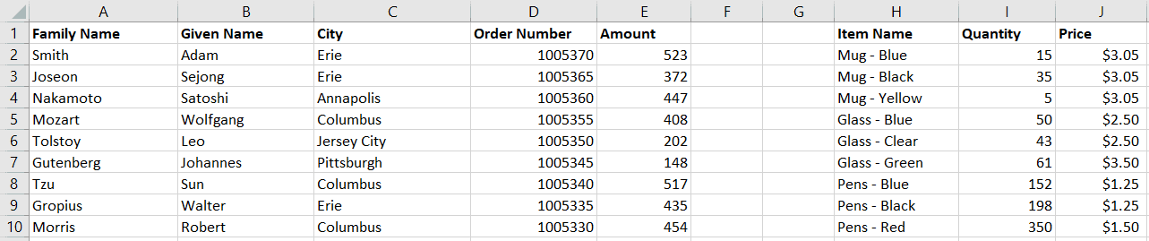
Example 1 — Using Range, Cells, Columns & Rows property — refer Image 1:

Sub CellsColumnsRowsProperty()
‘using Range, Cells, Columns & Rows property — refer Image 1:
Dim ws As Worksheet
Dim rng As Range
Dim r As Integer, c As Integer, n As Integer, i As Integer, j As Integer
‘set worksheet:
Set ws = Worksheets(«Sheet1»)
‘activate worksheet:
ws.activate
‘enter numbers starting from 1 in each row, for a 5 row & 5 column range (A1:E5):
For r = 1 To 5
n = 1
For c = 1 To 5
Cells(r, c).Value = n
n = n + 1
Next c
Next r
‘set range to A1:E5, wherein the numbers have been entered as above:
Set rng = Range(Cells(1, 1), Cells(5, 5))
‘set background color of each even number column to yellow and of each odd number column to green:
For i = 1 To 5
If i Mod 2 = 0 Then
rng.Columns(i).Interior.Color = vbYellow
Else
rng.Columns(i).Interior.Color = vbGreen
End If
Next i
‘set font color to red and set font to bold for of even number rows:
For j = 1 To 5
If j Mod 2 = 0 Then
rng.Rows(j).Font.Bold = True
rng.Rows(j).Font.Color = vbRed
End If
Next j
‘set font for all cells of the range to italics:
rng.Cells.Font.Italic = True
End Sub
To return the number of the first row in a range, use the Range.Row Property. If the specified range contains multiple areas, this property will return the number of the first row in the first area (Areas property has been explained in detail later in this section). Syntax: RangeObject.Row. To return the number of the first column in a range, use the Range.Column Property. If the specified range contains multiple areas, this property will return the number of the first column in the first area. Syntax: RangeObject.Column.
Examples:
Get the number of the first row in the specified range — returns 4:
MsgBox ActiveSheet.Range(«B4»).Row
MsgBox Worksheets(«Sheet1»).Range(«B4:D7»).Row
Get the number of the first column in the specified range — returns 2:
MsgBox ActiveSheet.Range(«B4:D7»).Column
Get the number of the last row in the specified range — returns 7:
Explanation: Range(«B4:D7»).Rows.Count returns 4 (the number of rows in the range). Range(«B4:D7»).Rows(Range(«B4:D7»).Rows.Count) or Range(«B4:D7»).Rows(4), returns the last row in the specified range.
MsgBox Range(«B4:D7»).Rows(Range(«B4:D7»).
Rows.Count).Row
Example 2: Using Row Property, Column Property & Rows Property, determine row number & column number, and alternate rows — refer Image 2.

Sub RowColumnProperty()
‘Using Row Property, Column Property & Rows Property, determine row number & column number, and alternate rows — refer Image 2.
Dim rng As Range, cell As Range
Dim i As Integer
Set rng = Worksheets(«Sheet1»).Range(«B4:D7»)
‘enter its row number & column number within each cell in the specified range:
For Each cell In rng
cell.Value = cell.Row & «,» & cell.Column
Next
‘set background color of each alternate row of the specified range:
For i = 1 To rng.Rows.count
If i Mod 2 = 1 Then
rng.Rows(i).Interior.Color = vbGreen
Else
rng.Rows(i).Interior.Color = vbYellow
End If
Next
End Sub
Also refer to Example 23, of using the End & Row properties to determine the last used row or column with data.
You can get a Range reference in vba language by using the Range.Address Property, which returns the address of a Range as a string value. This property is read-only.
Examples of using the Address Property:
Returns $B$2:
MsgBox Range(«B2»).Address
Returns $B$2,$C$3:
MsgBox Range(«B2,C3»).Address
Returns $A$1:$B$2,$C$3,$D$4:
Dim strRng As String
Range(«A1:B2,C3,D4»).Select
strRng = Selection.Address
MsgBox strRng
Returns $B2:
MsgBox Range(«B2»).Address(RowAbsolute:=False)
Returns B$2:
MsgBox Range(«B2»).Address(ColumnAbsolute:=False)
Returns R2C2:
MsgBox Range(«B2»).Address(ReferenceStyle:=xlR1C1)
Includes the worksheet (active sheet — «Sheet1») & workbook («Book1.xlsm») name, and returns [Book1.xlsm]Sheet1!$B$2:
MsgBox Range(«B2»).Address(External:=True)
Returns R[1]C[-1] — Range(«B2») is 1 row and -1 columns relative to Range(«C1»):
MsgBox Range(«B2»).Address(RowAbsolute:=False, ColumnAbsolute:=False, ReferenceStyle:=xlR1C1, RelativeTo:=Range(«C1»))
Returns RC[-2] — Range(«A1») is 0 row and -2 columns relative to Range(«C1»):
MsgBox Cells(1, 1).Address(RowAbsolute:=False, ColumnAbsolute:=False, ReferenceStyle:=xlR1C1, RelativeTo:=Range(«C1»))
Activate & Select Cells; the ActiveCell & Selection
The Select method (of the Range object) is used to select a cell or a range of cells in a worksheet — Syntax: RangeObject.Select. Ensure that the worksheet wherein the Select method is applied to select cells, is the active sheet. The ActiveCell Property (of the Application object) returns a single active cell (Range object) in the active worksheet. Remember that the ActiveCell property will not work if the active sheet is not a worksheet. When a cell(s) is selected in the active window, the Selection property (of the Application object) returns a Range object representing all cells which are currently selected in the active worksheet. A Selection may consist of a single cell or a range of multiple cells, but there will only be one active cell within it, which is returned by using the ActiveCell property. When only a single cell is selected, the ActiveCell property returns this cell. On selecting multiple cells using the Select method, the first referenced cell becomes the active cell, and thereafter you can change the active cell using the Activate method. Both the ActiveCell Property & the Selection property are read-only, and not specifying the Application object qualifier viz. Application.ActiveCell or ActiveCell, Application.Selection or Selection, will have the same effect. To activate a single cell within the current selection, use the Activate Method (of the Range object) — Syntax: RangeObject.Activate, and this activated cell is returned by using the ActiveCell property.
We have discussed above that a Selection may consist of a single cell or a range of multiple cells, whereas there can be only one active cell within the Selection. When you activate a cell outside the current selection, the activated cell becomes the only selected cell. You can also use the Activate method to specify a range of multiple cells, but in effect only a single cell will be activated, and this activated cell will be the top-left corner cell of the range specified in the method. If this top-left cell lies within the selection, the current selection will not change, but if this top-left cell lies outside the selection, then the specified range in the Activate method becomes the new selection.
See below codes which illustrate the concepts of ActiveCell and Selection.
Selection containing a range of cells, and the active cell:
‘selects range C1:F5:
Range(«C1:F5»).Select
‘returns C1, the first referenced cell, as the active cell:
MsgBox ActiveCell.Address
Selection containing a range of cells, and the active cell:
‘selects range C1:F5:
Range(«F5:C1»).Select
‘returns C1, the first referenced cell, as the active cell:
MsgBox ActiveCell.Address
Selection containing a range of cells, and the active cell:
‘selects range C1:F5:
Range(«C5:F1»).Select
‘returns C1, the first referenced cell, as the active cell:
MsgBox ActiveCell.Address
Activate a cell within the current selection:
‘selects range B6:F10:
Range(«B6:F10»).Select
‘returns B6, the first referenced cell, as the active cell:
MsgBox ActiveCell.Address
‘selection remains same — range B6:F10, but the active cell is now C8:
Range(«C8»).Activate
MsgBox ActiveCell.Address
Activate a cell outside the current selection:
‘selects range B6:F10:
Range(«B6:F10»).Select
‘returns B6, the first referenced cell, as the active cell:
MsgBox ActiveCell.Address
‘both the selection and the active cell is now A2:
Range(«A2»).Activate
MsgBox ActiveCell.Address
Select a cell within the current selection:
‘selects range B6:F10:
Range(«B6:F10»).Select
‘returns B6, the first referenced cell, as the active cell:
MsgBox ActiveCell.Address
‘both the selection and the active cell is now C8:
Range(«C8»).Select
MsgBox ActiveCell.Address
Activate a range of cells whose top-left cell is within the current selection:


‘selects range B6:F10 — refer Image 3a:
Range(«B6:F10»).Select
‘returns B6, the first referenced cell, as the active cell:
MsgBox ActiveCell.Address
‘selection remains same — range B6:F10, but the active cell is now C8 — refer Image 3b:
Range(«C8:G12»).Activate
MsgBox ActiveCell.Address
Activate a range of cells whose top-left cell is outside the current selection:

‘selects range B6:F10 — refer Image 3a:
Range(«B6:F10»).Select
‘returns B6, the first referenced cell, as the active cell:
MsgBox ActiveCell.Address
‘selection range changes to range B1:F8, and the active cell is now B1 — refer Image 3c:
Range(«B1:F8»).Activate
MsgBox ActiveCell.Address
Using the Application.Selection Property returns the selected object wherein the selection determines the returned object type. Where the selection is a range of cells, this property returns a Range object, and this Selection — which is a Range object — can comprise of a single cell, or multiple cells or multiple non-contiguous ranges. And as mentioned above, the Select method (of the Range object) is used to select a cell or a range of cells in a worksheet. Therefore, after selecting a range, you can perform actions on the selection of cells by using the Selection object. See below illustration.
Sub SelectionObject()
‘select cells in the active sheet using the Range.Select method:
Range(«A1:B3,D6»).Select
‘perform action (set interior color of cells to red) on the Selection, which is a Range object:
Selection.Interior.Color = vbRed
End Sub
Entire Row & Entire Column Properties, Inserting Cells/Rows/Columns using the Insert Method
Use the Range.EntireRow Property to return an entire row or rows within which the specific range is contained. Using this property returns a Range object referring to the entire row(s). Syntax: RangeObject.EntireRow. Use the Range.EntireColumn Property to return an entire column or columns within which the specific range is contained. Using this property returns a Range object referring to the entire column(s). Syntax: RangeObject.EntireColumn.
Examples of using the EntireRow & EntireColumn Properties
Selects row no. 2:
Range(«A2»).EntireRow.Select
Selects row nos. 2, 3 & 4:
Range(«A2:C4»).EntireRow.Select
Enters value 3 in range A3 ie. in the first cell of row no. 3:
Cells(3, 4).EntireRow.Cells(1, 1).Value = 3
Selects column A:
Range(«A2»).EntireColumn.Select
Selects columns A to C:
Range(«A2:C4»).EntireColumn.Select
Enters value 4 in range D1 ie. in the first cell of column no. 4:
Cells(3, 4).EntireColumn.Cells(1, 1).Value = 4
Use the Range.Insert Method to insert a cell or a range of cells in a worksheet. Syntax: RangeObject.Insert(Shift, CopyOrigin). Both arguments are optional to specify. When you insert cell(s) the other cells are shifted to make way, and you can set a value for the Shift argument to determine the direction in which the other cells are shifted — specifying xlShiftDown (value -4121) will shift the cells down, and xlShiftToRight (value -4161) shifts the cells to the right. Omitting this argument will decide the shift direction based on the shape of the range. Specifying xlFormatFromLeftOrAbove (value 0) for the CopyOrigin argument will copy the format for inserted cell(s) from the above cells or cells to the left, and specifying xlFormatFromRightOrBelow (value 1) will copy format from the below cells or cells to the right.
Illustrating Range.Insert Method — for start data refer Image 4a:


Shifts cells down and copies formatting of inserted cell from above cell — refer image 4b:
Range(«B2»).Insert

Shifts cells to the right and copies formatting of inserted cells from cells to the left — refer image 4c:
Range(«B2:C4»).Insert

Shifts cells down and copies formatting of inserted cells from above cells — refer image 4d:
Range(«B2:D3»).Insert

Shifts cells down and copies formatting of inserted cells from below cells — refer image 4e:
Range(«B2:D3»).Insert CopyOrigin:=xlFormatFromRightOrBelow

Shifts cells to the right and copies formatting of inserted cells from cells to the left — refer image 4f:
Range(«B2:D3»).Insert shift:=xlShiftToRight

Shifts cells to the right and copies formatting of inserted cells from cells to the right — refer image 4g:
Range(«B2:D3»).Insert shift:=xlShiftToRight, CopyOrigin:=xlFormatFromRightOrBelow

Inserts 2 rows — row no 2 & 3 — and copies formatting of inserted rows from above cells — refer image 4h:
Range(«B2:D3»).EntireRow.Insert
Below are some illustrations of inserting entire row(s) or column(s) dynamically in a worksheet.
Example 3: Insert row or column — specify the row / column to insert.
Sub InsertRowColumn()
‘Insert row or column — specify the row / column to insert:
Dim ws As Worksheet
Set ws = Worksheets(«Sheet1»)
‘NOTE: each of the below codes need to be run individually.
‘specify the exact row number to insert — insert a row as row no 12:
ws.Rows(12).Insert
‘specify the range below which to insert a row — insert a row below range C3 ie. as row no 4.
ws.Range(«C3»).EntireRow.Offset(1, 0).Insert
‘specify the exact column number to insert — insert a column as column no 4:
ws.Columns(4).Insert
‘specify the range to the right of which to insert a column — insert a column to the right of range C3 ie. as column no 4.
ws.Range(«C3»).EntireColumn.Offset(0, 1).Insert
End Sub
Example 4: Insert row(s) after a specified value is found.
Sub InsertRow1()
‘insert row(s) after a specified value is found:
Dim ws As Worksheet
Dim rngFind As Range, rngSearch As Range, rngLastCell As Range
Dim lFindRow As Long
Set ws = Worksheets(«Sheet1»)
‘find a value after which to insert a row:
Set rngSearch = ws.Range(«A1:E100»)
‘begin search AFTER the last cell in search range (this will start serach from the first cell in search range):
Set rngLastCell = rngSearch.Cells(rngSearch.Cells.count)
Set rngFind = rngSearch.Find(What:=«ExcelVBA», After:=rngLastCell, LookIn:=xlValues, lookat:=xlWhole)
‘exit procedure if value not found:
If Not rngFind Is Nothing Then
lFindRow = rngFind.Row
MsgBox lFindRow
Else
MsgBox «Value not found!»
Exit Sub
End If
‘NOTE: each of the below codes need to be run individually.
‘if value found is in row no 12, one row will be inserted below as row no 13:
ws.Cells(lFindRow + 1, 1).EntireRow.Insert
‘if value found is in row no 12, one row will be inserted 3 rows below (as row no 15):
ws.Cells(lFindRow + 3, 1).EntireRow.Insert
‘if value found is in row no 12, one row will be inserted 3 rows below (as row no 15):
ws.Cells(lFindRow, 1).Offset(3).EntireRow.Insert
‘if value found is in row no 12, 3 rows will be inserted above (as row nos 12, 13 & 14) and the value found row 12 will be pushed down to row 15:
ws.Cells(lFindRow, 1).EntireRow.Resize(3).Insert
‘alternate:
ws.Range(Cells(lFindRow, 1), Cells(lFindRow + 2, 1)).EntireRow.Insert
‘alternate:
ws.Rows(lFindRow & «:» & lFindRow + 2).EntireRow.Insert Shift:=xlDown
‘if value found is in row no 12, 3 rows will be inserted below (as row nos 13, 14 & 15) and the value found row 12 will remain at the same position:
ws.Cells(lFindRow + 1, 1).EntireRow.Resize(3).Insert
‘alternate:
ws.Range(ws.Cells(lFindRow + 1, 1), ws.Cells(lFindRow + 3, 1)).EntireRow.Insert
‘if value found is in row no 12, 3 rows will be inserted after row no 13 (as row nos 14, 15 & 16) and existing rows 12 & 13 will remain at the same position:
ws.Cells(lFindRow + 2, 1).EntireRow.Resize(3).Insert
End Sub
Example 5: Insert a row, n rows above the last used row.
Sub InsertRow2()
‘insert a row, n rows above the last used row
Dim ws As Worksheet
Dim lRowsC As Long
Set ws = Worksheets(«Sheet1»)
‘determine the last used row in a column (column A):
lRowsC = ws.Cells(Rows.count, «A»).End(xlUp).Row
MsgBox lRowsC
‘set n to the no of rows above the last used row:
n = 5
‘check if there are enough rows before the last used row, else you will get an error:
If lRowsC >= n Then
‘insert a row, n rows above the last used row — if last used row is no 5 before insertion, then insert as row no 1 and the last used row will become no 6 (similarly, if last used row is 27, then insert as row no 23) :
ws.Rows(lRowsC).Offset(-n + 1, 0).EntireRow.Insert
Else
MsgBox «Not enough rows before the last used row!»
End If
End Sub
Example 6: Insert a row each time the searched value is found in a range.
For live code of this example, click to download excel file.
Sub InsertRow3()
‘search value in a range and insert a row each time the value is found.
‘you can set the search range with the variable rngSearch in below code — the code will look within this range to find the value below which row is to be inserted.
Dim ws As Worksheet
Dim rngFind As Range, rngSearch As Range, rngLastCell As Range
Dim strAddress As String
Set ws = Worksheets(«Sheet1»)
‘set search range:
Set rngSearch = ws.Range(«A1:K100»)
MsgBox «Searching for ‘ExcelVBA’ within range: » & rngSearch.Address
‘begin search AFTER the last cell in search range
Set rngLastCell = rngSearch.Cells(rngSearch.Cells.count)
‘find value in specified range, starting search AFTER the last cell in search range:
Set rngFind = rngSearch.Find(What:=«ExcelVBA», After:=rngLastCell, LookIn:=xlValues, lookat:=xlWhole)
If rngFind Is Nothing Then
MsgBox «Value not found!»
Exit Sub
Else
‘save cell address of first value found:
strAddress = rngFind.Address
Do
‘find next occurrence of value:
Set rngFind = rngSearch.FindNext(After:=rngFind)
‘insert row below when value is found (if value is found twice in a row, then 2 rows will be inserted):
rngFind.Offset(1).EntireRow.Insert
‘loop till reaching the first value found range:
Loop While rngFind.Address <> strAddress
End If
End Sub
Example 7: Insert rows (user-defined number) within consecutive values found in a column — refer Images 5a & 5b.
For live code of this example, click to download excel file.


Sub InsertRow4()
‘insert rows (user-defined number) wherever 2 consecutive values are found in a column.
‘set column number in which 2 consecutive values are checked to insert rows, using the variable lCellColumn in below code.
‘set row number from where to start searching consecutive values, using the variable lCellRow in below code.
‘refer Image 5a which shows raw data, and Image 5b after this procedure is executed — a single row (lRowsInsert value entered as 1 in input box) is inserted where consecutive values appear in column 1:
Dim ws As Worksheet
Dim lLastUsedRow As Long, lRowsInsert As Long, lCellRow As Long, lCellColumn As Long
Dim rng As Range
Set ws = Worksheets(«Sheet1»)
ws.Activate
‘set column number in which 2 consecutive values are checked to insert rows:
lCellColumn = 1
‘set row number from where to start searching consecutive values:
lCellRow = 1
‘determine the last used row in the column (column no. lCellColumn):
lLastUsedRow = Cells(Rows.count, lCellColumn).End(xlUp).Row
‘enter number of rows to insert between 2 consecutive values:
lRowsInsert = InputBox(«Enter number of rows to insert»)
If lRowsInsert < 1 Then
MsgBox «Error — please enter a value equal to or greater than 1»
Exit Sub
End If
MsgBox «This code will insert » & lRowsInsert & » rows, wherever consecutive values are found in column number » & lCellColumn & «, starting search from row number » & lCellRow
‘loop till the row number equals the last used row (ie. loop right till the end value in the column):
Do While lCellRow < lLastUsedRow
Set rng = Cells(lCellRow, lCellColumn)
‘in case of 2 consecutive values:
If rng <> «» And rng.Offset(1, 0) <> «» Then
‘enter the user-defined number of rows:
Range(rng.Offset(1, 0), rng.Offset(lRowsInsert, 0)).EntireRow.Insert
lCellRow = lCellRow + lRowsInsert + 1
‘determine the last used row — it is dynamic and changes on insertion of rows:
lLastUsedRow = Cells(Rows.count, lCellColumn).End(xlUp).Row
‘alternate method to determine the last used row, when number of rows inserted is fixed — this is faster than using End(xlUp):
‘lLastUsedRow = lLastUsedRow + lRowsInsert + 1
‘MsgBox lLastUsedRow
Else
lCellRow = lCellRow + 1
End If
Loop
End Sub