
Add time
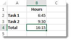
Suppose that you want to know how many hours and minutes it will take to complete two tasks. You estimate that the first task will take 6 hours and 45 minutes and the second task will take 9 hours and 30 minutes.
Here is one way to set this up in the a worksheet.
-
Enter 6:45 in cell B2, and enter 9:30 in cell B3.
-
In cell B4, enter =B2+B3 and then press Enter.

The result is 16:15—16 hours and 15 minutes—for the completion the two tasks.
Tip: You can also add up times by using the AutoSum function to sum numbers. Select cell B4, and then on the Home tab, choose AutoSum. The formula will look like this: =SUM(B2:B3). Press Enter to get the same result, 16 hours and 15 minutes.
Well, that was easy enough, but there’s an extra step if your hours add up to more than 24. You need to apply a special format to the formula result.
To add up more than 24 hours:
-
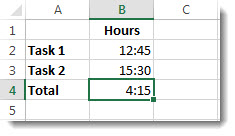
In cell B2 type 12:45, and in cell B3 type 15:30.
-
Type =B2+B3 in cell B4, and then press Enter.
The result is 4:15, which is not what you might expect. This is because the time for Task 2 is in 24-hour time. 15:30 is the same as 3:30.
-
To display the time as more than 24 hours, select cell B4.
-
On the Home tab, in the Cells group, choose Format, and then choose Format Cells.
-
In the Format Cells box, choose Custom in the Category list.
-
In the Type box, at the top of the list of formats, type [h]:mm;@ and then choose OK.
Take note of the colon after [h] and a semicolon after mm.

The result is 28 hours and 15 minutes. The format will be in the Type list the next time you need it.
Subtract time
Here’s another example: Let’s say that you and your friends know both your start and end times at a volunteer project, and want to know how much time you spent in total.
Follow these steps to get the elapsed time—which is the difference between two times.
-
In cell B2, enter the start time and include “a” for AM or “p” for PM. Then press Enter.
-
In cell C2, enter the end time, including “a” or “p” as appropriate, and then press Enter.
-
Type the other start and end times for your friends, Joy and Leslie.
-
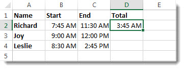
In cell D2, subtract the end time from the start time by entering the formula =C2-B2, and then press Enter.
-
In the Format Cells box, click Custom in the Category list.
-
In the Type list, click h:mm (for hours and minutes), and then click OK.
Now we see that Richard worked 3 hours and 45 minutes.
-
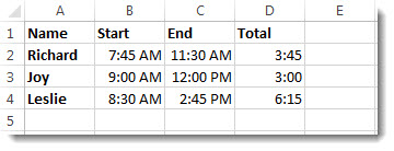
To get the results for Joy and Leslie, copy the formula by selecting cell D2 and dragging to cell D4.
The formatting in cell D2 is copied along with the formula.
To subtract time that’s more than 24 hours:
It is necessary to create a formula to subtract the difference between two times that total more than 24 hours.
Follow the steps below:
-
Referring to the above example, select cell B1 and drag to cell B2 so that you can apply the format to both cells at the same time.
-
In the Format Cells box, click Custom in the Category list.
-
In the Type box, at the top of the list of formats, type m/d/yyyy h:mm AM/PM.
Notice the empty space at the end of yyyy and at the end of mm.
The new format will be available when you need it in the Type list.
-
In cell B1, type the start date, including month/day/year and time using either “a” or “p” for AM and PM.
-
In cell B2, do the same for the end date.
-
In cell B3, type the formula =(B2-B1)*24.
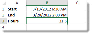
The result is 31.5 hours.
Note: You can add and subtract more than 24 hours in Excel for the web but you cannot apply a custom number format.
Add time
Suppose you want to know how many hours and minutes it will take to complete two tasks. You estimate that the first task will take 6 hours and 45 minutes and the second task will take 9 hours and 30 minutes.
-
In cell B2 type 6:45, and in cell B3 type 9:30.
-
Type =B2+B3 in cell B4, and then press Enter.
It will take 16 hours and 15 minutes to complete the two tasks.
Tip: You can also add up times using AutoSum. Click in cell B4. Then click Home > AutoSum. The formula will look like this: =SUM(B2:B3). Press Enter to get the result, 16 hours and 15 minutes.
Subtract time
Say you and your friends know your start and end times at a volunteer project, and want to know how much time you spent. In other words, you want the elapsed time or the difference between two times.
-
In cell B2 type the start time, enter a space, and then type “a” for AM or “p” for PM, and press Enter. In cell C2, type the end time, including “a” or “p” as appropriate, and press Enter. Type the other start and end times for your friends Joy and Leslie.
-
In cell D2, subtract the end time from the start time by typing the formula: =C2-B2, and then pressing Enter. Now we see that Richard worked 3 hours and 45 minutes.
-
To get the results for Joy and Leslie, copy the formula by clicking in cell D2 and dragging to cell D4. The formatting in cell D2 is copied along with the formula.
 Dates and times are two of the most common data types people work with in Excel, but they are also possibly the most frustrating to work with, especially if you are new to Excel and still learning. This is because Excel uses a serial number to represent the date instead of a proper month, day, or year, nevermind hours, minutes, or seconds. It’s made more complicated by the fact that dates are also days of the week, like Monday or Friday, even though Excel doesn’t explicitly store that information in the cells. Here is the definitive guide to working with dates and times in Excel…
How Excel Stores Dates
The source of most of the confusion around dates and times in Excel comes from the way that the program stores the information. You’d expect it to remember the month, the day, and the year for dates, but that’s not how it works…
Excel stores dates as a serial number that represents the number of days that have taken place since the beginning of the year 1900. This means that January 1, 1900 is really just a 1. January 2, 1900 is 2. By the time we get all the way to the present decade, the numbers have gotten pretty big… September 10, 2013 is stored as 41527.
Importantly, any date before January 1, 1900 is not recognized as a date in Excel. There are no “negative” date serial numbers on the number line.
It seems confusing, but it makes it a lot easier to add, subtract, and count days. A week from September 10, 2013 (September 17, 2013), is just 41527 + 7 days, or 41534.
How Excel Stores Times
Excel stores times using the exact same serial numbering format as with dates. Days start at midnight (12:00am or 0:00 hours). Since each hour is 1/24 of a day, it is represented as that decimal value: 0.041666…
That means that 9:00am (09:00 hours) on September 10, 2013 will be stored as 41527.375.
When a time is specified without a date, Excel stores it as if it occurred on January 0, 1900. In other words, 3:00pm (15:00 hours) is stored as 0.625. This can make doing math for time-only values (that have no date) challenging, since subtracting 6 hours (6:00) from 3:00am (03:00 hours) will become negative and count as an error: 0.125 – 0.25 = -0.125, which is displayed as #########.
Minutes and seconds in Excel work the same way as hours…
A minute is 1/60 of an hour, which is 1/24 of a day, or 1/1440 of a day in total, which calculates to 0.00069444…
A second is 1/60 of an minute, which is 1/60 of an hour, which is 1/24 of a day, or 1/86400 of a day in total, which calculates to 0.00001157407…
Working with Dates and Times
DATE() and TIME()
Serial numbers aren’t all that intuitive to use. Fortunately, Excel has a set of functions to make it easier to find and use dates and times, starting with DATE and TIME. The syntax is as follows:
=DATE(year, month, day)
=TIME(hours, minutes, seconds)
For both functions, specify the year, month, and day, or hours, minutes, and seconds as numbers. For example, September 10, 2013 can be entered as:
=DATE(2013,9,10)
It will be stored as 41527, which means that it is technically storing 12:00am on September 10, 2013.
For times, 6:00pm (18:00 hours) can be entered as:
=TIME(18,0,0)
It will be stored as 0.75, which means that it is technically storing 6:00pm on January 0, 1900.
If we want to represent a specific time and date, we can add the two functions together. For example, 6:00pm (18:00 hours) on September 10, 2013 can be entered as:
=DATE(2013,9,10)+TIME(18,0,0)
It will be calculate as 41527.75, which means Excel is storing exactly the date we want…
Additional Date and Time Setting Functions
Excel has a few additional functions to make declaring dates easier.
TODAY()
The TODAY function always returns the current date’s serial number. The TODAY function is just entered as:
=TODAY()
This article was written at 6:30pm (18:30 hours) on September 24, 2013, and the TODAY function calculated to 41541. That means that it is technically storing 12:00am on September 24, 2013.
NOW()
A similar function called NOW always returns the current date and time’s serial number. The NOW function is just entered as:
=NOW()
Again, at 6:30pm (18:30 hours) on September 24, 2013, the function calculated to 41541.77081333… NOW stores the exact time and date, down to the second.
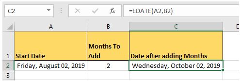
EDATE() and EOMONTH()
The EDATE function gives the date the specified number of months away from the input date. The EOMONTH function gives the date of the last day of the month. It can do so for the current month or a number of months in the future or the past. The syntax for each is as follows:
=EDATE(start_date, months)
=EOMONTH(start_date, months)
The start_date can be any date-formatted cell reference or date serial number.
The months field can be any number, though only the integer value will be used (e.g. it treats 2.8 as 2).
The EDATE and EOMONTH functions strip the time value from the date. For example, For example, if cell A1 stores September 10, 2013, we can get the value 2 months ahead as follows:
=EDATE(A1,2)
Returns 12:00am (0:00 hours) on November 10, 2013, or 41588. This function works even though the months have different numbers of days (September and November have 30, October has 31).
=EOMONTH(A1,2)
Returns 12:00am (0:00 hours) on November 30, 2013, or 41588. Again, this function works even though the months have different numbers of days.
WORKDAY()
Occasionally, it may be useful to count ahead based on work-days (Monday-Friday) instead of all 7 days of the week… For that, Excel has provided WORKDAY. The syntax for WORKDAY is as follows:
=WORKDAY(start_date, days, [holidays])
The start_date is as above.
The days input is the number of workdays ahead (or behind) of the present day you would like to move.
The [holidays] input is optional, but lets you disqualify specific days (like Thanksgiving or Christmas, for example), which might otherwise fall during the work week. These are date serial numbers provided in an array bounded by brackets: { }. To specify multiple holidays, the dates must be held in cells – it is not possible to put multiple DATE functions in an array.
For example, let’s find the date 6 work days before 6:00pm (18:00 hours) on September 10, 2013 (stored in cell A1). Monday, September 2nd is Labor Day, so let’s include that as a holiday:
=WORKDAY(A1,-6,DATE(2013,9,2))
Returns 12:00am (0:00 hours) on August 30, 2013, or 41516. (Note that the function strips the time portion of the date.)
WORKDAY.INTL() (Excel 2010 and newer)
For newer versions of Excel (2010 and later), there is another version of WORKDAY called WORKDAY.INTL. WORKDAY.INTL works just like WORKDAY, but it adds the ability to customize the definition of the “weekend”. The syntax for WORKDAY.INTL is as follows:
=WORKDAY.INTL(start_date, days, [weekend], [holidays])
The start_date, days, and [holidays] inputs work just like the normal WORKDAY function.
The [weekend] input has the following options:
Retrieving Dates in Excel
DAY(), MONTH(), and YEAR()
Now we know how define dates, but we still need to be able to work with them. Serial numbers don’t make it easy to extract months, years, and days, nevermind hours, minutes, and seconds. That’s why Excel has specific functions for pulling out each of these values. For working with the calendar, there is DAY, MONTH, and YEAR. The syntax is simple:
=DAY(serial_number)
=MONTH(serial_number)
=YEAR(serial_number)
The serial_number in each can be any date-formatted cell reference. For example, if cell A1 stores September 10, 2013, we can use each of the formulas in turn:
=DAY(A1)
Returns 10 as a numeric value.
=MONTH(A1)
Returns 9 as a numeric value.
=YEAR(A1)
Returns 2013 as a numeric value.
We could have also given the direct serial number for September 10, 2013:
=DAY(41527)
Returns 10 as a numeric value.
Retrieving Times in Excel
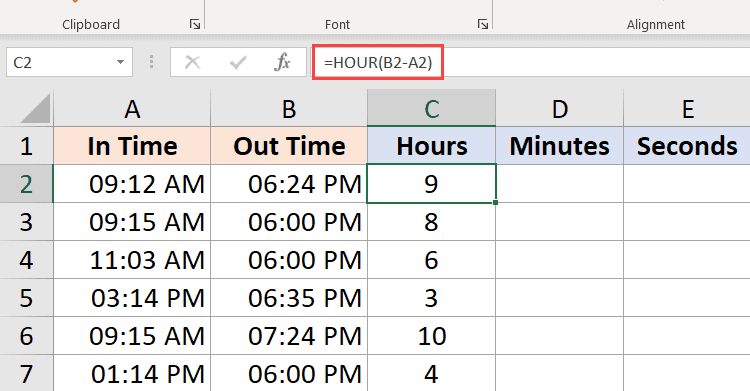
HOUR(), MINUTE(), and SECOND()
For times, the process is very similar. Excel has function to retrieve the hours, minutes, and seconds from a time stamp, conveniently named HOUR, MINUTE, and SECOND. The syntax is identical:
=HOUR(serial_number)
=MINUTE(serial_number)
=SECOND(serial_number)
The serial_number in each can be any time/date-formatted cell reference. For example, if A1 stores 6:15:30pm (18:15 hours, 30 seconds) on September 10, 2013, we can use each of the formulas in turn:
=HOUR(A1)
Returns 18 as a numeric value.
=MINUTE(A1)
Returns 15 as a numeric value.
=SECOND(A1)
Returns 30 as a numeric value.
We could have also given the direct serial number for 6:15:30pm (18:15 hours, 30 seconds) on September 10, 2013:
=SECOND(41527.7607638889)
Returns 30 as a numeric value.
Additional Date Retrieving Functions
WEEKDAY() and WEEKNUM()
Dates don’t just have month and year information. They also encode indirect information… September 10, 2013 happens to also be a Tuesday. Excel has a few of functions to work with the week aspect of dates: WEEKDAY and WEEKNUM. The syntax is as follows:
=WEEKDAY(serial_number, [return_type])
=WEEKNUM(serial_number, [return_type])
The serial_number in each can be any date-formatted cell reference. Since [return_type] is optional, each function assumes that each week starts on Sunday. If cell A1 stores September 10, 2013 (a Tuesday), we can use each of the formulas in turn:
=WEEKDAY(A1)
Returns 3, since Tuesday is the 3rd day of a week that starts on Sunday.
=WEEKNUM(A1)
Returns 37, since September 10, 2013 is in the 37th week of 2013, when you start counting weeks from Sunday.
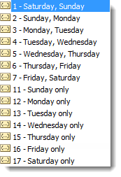
The [return_type] allows you to specify a different default week arrangement. You could let the week start on Monday and run until Sunday, or Saturday until Friday, for example. Excel is annoying, however, and makes the entry different for WEEKDAY and WEEKNUM. The full list of options for WEEKDAY is as follows:
Options 2 and 11 are functionally the same – the first is just there for backwards compatibility with earlier versions of Excel.
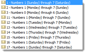
The full list of options for WEEKNUM is as follows:
Counting and Tracking Dates
Dates can be added and subtracted like normal numbers because they’re stored as serial numbers. That lets you count the days between two different dates. Sometimes, though, you need to count by a different metric.
NETWORKDAYS()
Above, we learned about WORKDAY, which lets you move back and forth a set number of workdays, ignoring weekends and holidays. But what if you need to measure the number of workdays between two dates? For that, Excel provides NETWORKDAYS. The formula syntax is as follows:
=NETWORKDAYS(start_date, end_date, [holidays])
The start_date and end_date can be any date-formatted cell reference.
The [holidays] input is optional, but lets you disqualify specific days (like Thanksgiving or Christmas, for example), which might otherwise fall during the work week. These are date serial numbers provided in an array bounded by brackets: { }. To specify multiple holidays, the dates must be held in cells – it is not possible to put multiple DATE functions in an array.
For example, if A1 contains 6:00pm (18:00 hours) on September 10, 2013 and B1 contains 9:00am (9:00 hours) on December 2, 2013, we can use NETWORKDAYS to find the number of workdays between the two dates.
Let’s exclude Columbus Day (October 14, 2013), Veterans Day (November 11, 2013), and Thanksgiving Day (November 28, 2013) as holidays. To do so, we have to store those dates in other cells. Let’s put them in C1, C2, and C3:
=DATE(2013,10,14)
=DATE(2013,11,11)
=DATE(2013,11,28)
Now, we can combine them in the function:
=NETWORKDAYS(A1,B1,C1:C3)
The function returns 57 as a numeric value.
NETWORKDAYS.INTL() (Excel 2010 and newer)
For newer versions of Excel (2010 and later), there is another version of NETWORKDAYS called NETWORKDAYS.INTL. NETWORKDAYS.INTL works just like NETWORKDAYS, but it adds the ability to customize the definition of the “weekend”. The syntax for NETWORKDAYS.INTL is as follows:
=NETWORKDAYS.INTL(start_date, end_date, [weekend], [holidays])
The start_date, end_date, and [holidays] inputs work just like the normal WORKDAY function.
The [weekend] input has the following options:
YEARFRAC()
Sometimes it’s useful to measure how much time has passed in years, but subtracting the YEAR function will only round down to the nearest full year. YEARFRAC takes two dates and provides the portion of the year between them. The syntax is as follows:
=YEARFRAC(start_date, end_date, [basis])
The start_date and end_date can be any date-formatted cell reference.
The [basis] input is optional, but lets you specify the “rules” for measuring the difference. Most of the time, you’ll want to use option 1, but here is the full list:
 For example, if A1 contains September 10, 2013 and B1 contains December 2, 2013, we can use YEARFRAC to find the decimal portion of a year between the two dates:
=YEARFRAC(A1,B1,1)
Returns 0.227397260273973.
DATEDIF() (Undocumented Function)
The YEARFRAC function gives you the difference between dates as a fraction of a year, but sometimes you need more control. There is a powerful hidden function in Excel called DATEDIF that can do much more. It can tell you the number of years, months, or days between two dates. It can also track based on only partial inputs, ignoring years or months when calculating days. The syntax for DATEDIF is as follows:
=DATEDIF(start_date, end_date, unit)
The start_date and end_date can be any date-formatted cell reference.
The unit input asks you to specify a string that represents the type of output you want. This is slightly cumbersome, since you must wrap the input in quotes (” “).
For example, if A1 contains September 10, 2012 and B1 contains December 2, 2013, we can use DATEDIF to find the number of full years between the two dates:
=DATEDIF(A1,B1,"Y")
Returns 1 as a numeric value.
Using the same start_date and end_date inputs, here are the output possibilities for DATEDIF using different unit parameters:
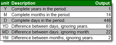
Every time, the unit must be put in quotes (e.g. “Y” or “MD”).
Converting Dates and Times from Text
DATEVALUE() and TIMEVALUE()
All of the above functions work perfectly with date-formatted serial numbers in Excel. Unfortunately, dates and times are often imported into worksheets as text. Most of the assorted functions like MONTH and HOUR are reasonably intelligent about converting on the fly. Occasionally it’s useful to build a date value through concatenation. The two functions Excel provides for this purpose are DATEVALUE and TIMEVALUE. The syntax for each is as follows:
=DATEVALUE(date_text)
=TIMEVALUE(time_text)
The date_text and time_text accept any text string that looks like a date or time.
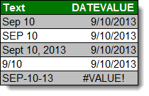
This is how DATEVALUE responds to various date_text inputs:
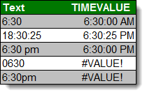
This is how TIMEVALUE responds to various time_text inputs:
Converting Dates and Times to Text
TEXT()
Getting data converted to dates and times is great, but you may also need to get it back out. Sometimes, you need a special format. Other times, you need to look for a date in a text string, and have to match using string tools like FIND and SEARCH. There is one master function for converting dates and times to text strings in Excel, called TEXT. The syntax for TEXT is as follows:
=TEXT(value, format_text)
The value can be any date or time-formatted cell reference.
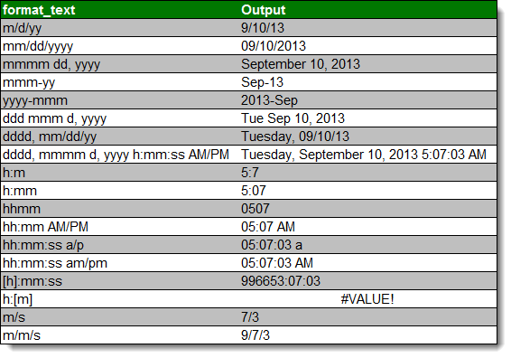
The format_text input has a large number of options, summarized here:
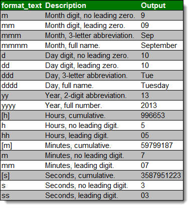
The outputs can be combined with simple formatting characters to produce standard date formats. Using the date 5:07:03am (05:07 hours, 3 seconds) on September 10, 2013, here are examples of possible outputs:
A Common Problem
One issue people frequently run into is that Excel occasionally misinterprets text fields as dates. An example is here:
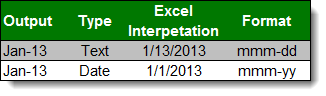
Be careful when entering dates, especially if you are importing from other data sources, to make sure that your “Jan-13” is being stored as January 1, 2013 and not January 13, 2013!
Get the latest Excel tips and tricks by joining the newsletter!
 Andrew Roberts has been solving business problems with Microsoft Excel for over a decade. Excel Tactics is dedicated to helping you master it.
Join the newsletter to stay on top of the latest articles. Sign up and you’ll get a free guide with 10 time-saving keyboard shortcuts!
Other posts in this series…
Since dates and times are stored as numbers in the back end in Excel, you can easily use simple arithmetic operations and formulas on the date and time values.
For example, you can add two different time values or date values or you can calculate the time difference between two given dates/times.
In this tutorial, I will show you a couple of ways to perform calculations using time in Excel (such as calculating the time difference, adding or subtracting time, showing time in different formats, and doing a sum of time values)
How Excel Handles Date and Time?
As I mentioned, dates and times are stored as numbers in a cell in Excel. A whole number represents a complete day and the decimal part of a number would represent the part of the day (which can be converted into hours, minutes, and seconds values)
For example, the value 1 represents 01 Jan 1900 in Excel, which is the starting point from which Excel starts considering the dates.
So, 2 would mean 02 Jan 1990, 3 would mean 03 Jan 1900 and so on, and 44197 would mean 01 Jan 2021.
Note: Excel for Windows and Excel for Mac follow different starting dates. 1 in Excel for Windows would mean 1 Jan 1900 and 1 in Excel for Mac would mean 1 Jan 1904
If there are any digits after a decimal point in these numbers, Excel would consider those as part of the day and it can be converted into hours, minutes, and seconds.
For example, 44197.5 would mean 01 Jan 2021 12:00:00 PM.

So if you’re working with time values in Excel, you would essentially be working with the decimal portion of a number.
And Excel gives you the flexibility to convert that decimal portion into different formats such as hours only, minutes only, seconds only, or a combination of hours, minutes, and seconds
Now that you understand how time is stored in Excel, let’s have a look at some examples of how to calculate the time difference between two different dates or times in Excel
Formulas to Calculating Time Difference Between Two Times
In many cases, all you want to do is find out the total time that has elapsed between the two-time values (such as in the case of a timesheet that has the In-time and the Out-time).
The method you choose would depend on how the time is mentioned in a cell and in what format you want the result.
Let’s have a look at a couple of examples
Simple Subtraction of Calculate Time Difference in Excel
Since time is stored as a number in Excel, find the difference between 2 time values, you can easily subtract the start time from the end time.
End Time – Start Time
The result of the subtraction would also be a decimal value that would represent the time that has elapsed between the two time-values.
Below is an example where I have the start and the end time and I have calculated the time difference with a simple subtraction.

There is a possibility that your results are shown in the time format (instead of decimals or in hours/minutes values). In our above example, the result in cell C2 shows 09:30 AM instead of 9.5.
That’s perfectly fine as Excel tries to copy the format from the adjacent column.
To convert this into a decimal, change the format of the cells to General (the option is in the Home tab in the Numbers group)
Once you have the result, you can format it in different ways. For example, you can show the value in hours only or minutes only or a combination of hours, minutes, and seconds.
Below are the different formats you can use:
| Format | What it Does |
| h | Shows only the hours elapsed between the two dates |
| hh | Shows hours in double-digit (such as 04 or 12) |
| hh:mm | Shows hours and minutes elapsed between the two dates, such as 10:20 |
| hh:mm:ss | Shows hours, minutes, and seconds elapsed between the two dates, such as 10:20:36 |
And if you’re wondering where and how to apply these custom date formats, follow the below steps:
- Select the cells where you want to apply the date format
- Hold the Control key and press the 1 key (or Command + 1 if using Mac)
- In the Format Cells dialog box that opens, click on the Number tab (if not selected already)

- In the left pane, click on Custom
- Enter any of the desired format code in the Type field (in this example, I am using hh:mm:ss)
- Click OK


The above steps would change the formatting and show you the value based on the format.

Note that custom number formatting does not change the value in the cell. It only changes the way a value is being displayed. So, I can choose to only show the hour value in a cell, while it would still have the original value.
Pro tip: If the total number of hours exceeds 24 hours, use the following custom number format instead: [hh]:mm:ss
Calculate the Time Difference in Hours, Minutes, or Seconds
When you subtract the time values, Excel returns a decimal number that represents the resulting time difference.
Since every whole number represents one day, the decimal part of the number would represent that much part of the day which can easily be converted into hours or minutes, or seconds.
Calculating Time Difference in Hours
Suppose you have the dataset as shown below and you want to calculate the number of hours between the two-time values

Below is the formula that will give you the time difference in hours:
=(B2-A2)*24
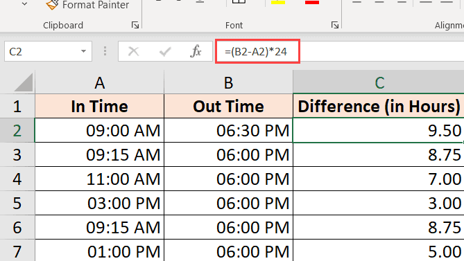
The above formula will give you the total number of hours elapsed between the two-time values.
Sometimes, Excel tries to be helpful and will give you the result in time format as well (as shown below).

You can easily convert this into Number format by clicking on the Home tab, and in the Number group, selecting Number as the format.

If you only want to return the total number of hours elapsed between the two times (without any decimal part), use the below formula:
=INT((B2-A2)*24)

Note: This formula only works when both the time values are of the same day. If the day changes (where one of the time values is of another date and the second one of another date), This formula will give wrong results. Have a look at the section where I cover the formula to calculate the time difference when the date changes later in this tutorial.
Calculating Time Difference in Minutes
To calculate the time difference in minutes, you need to multiply the resulting value by the total number of minutes in a day (which is 1440 or 24*60).
Suppose you have a data set as shown below and you want to calculate the total number of minutes elapsed between the start and the end date.
Below is the formula that will do that:
=(B2-A2)*24*60

Calculating Time Difference in Seconds
To calculate the time difference in seconds, you need to multiply the resulting value by the total number of seconds in a day (which is or 24*60*60 or 86400).
Suppose you have a data set as shown below and you want to calculate the total number of seconds that have elapsed between the start and end date.
Below is the formula that will do that:
=(B2-A2)*24*60*60

Calculating time difference with the TEXT function
Another easy way to quickly get the time difference without worrying about changing the format is to use the TEXT function.
The TEXT function allows you to specify the format right within the formula.
=TEXT(End Date - Start Date, Format)
The first argument is the calculation you want to do, and the second argument is the format in which you want to show the result of the calculation.
Suppose you have a dataset as shown below and you want to calculate the time difference between the two times.
Here are some formulas that will give you the result with different formats
Show only the number of hours:
=TEXT(B2-A2,"hh")

The above formula will only give you the result that shows the numbers of hours elapsed between the two-time values. If your result is 9 hours and 30 minutes, it will still show you 9 only.
Show the number of total minutes
=TEXT(B2-A2,"[mm]")

Show the number of total seconds
=TEXT(B2-A2,"[ss]")

Show Hours and Minutes
=TEXT(B2-A2,"[hh]:mm")

Show Hours, Minutes, and Seconds
=TEXT(B2-A2,"hh:mm:ss")

If you’re wondering what’s the difference between hh and [hh] in the format (or mm and [mm]), when you use the square brackets, it would give you the total number of hours between the two dates, even if the hour value is higher than 24. So if you subtract two date values where the difference is more than24 hours, using [hh] will give you the total number of hours and hh will only give you the hours elapsed on the day of the end date.
Get the Time Difference in One-Unit (Hours/Minutes) and Ignore Others
If you want to calculate the time difference between the two time-values in only the number of hours or minutes or seconds, then you can use the dedicated HOUR, MINUTE, or SECOND function.
Each of these functions takes one single argument, which is the time value, and returns the specified time unit.
Suppose you have a data set as shown below, and you want to calculate the total number of hours minutes, and seconds that have elapsed between these two times.

Below are the formulas to do this:
Calculating Hours Elapsed Between two times
=HOUR(B2-A2)
Calculating Minutes from the time value result (excluding the completed hours)
=MINUTE(B2-A2)

Calculating Seconds from the time value result (excluding the completed hours and minutes)
=SECOND(B2-A2)

A couple of things that you need to know when working with these HOURS, MINUTE, and SECOND formulas:
- The difference between the end time and the start time cannot be negative (which is often the case when the date changes). In such cases, these formulas would return a #NUM! error
- These formulas only use the time portion of the resulting time value (and ignore the day portion). So if the difference in the end time and the start time is 2 Days, 10 Hours, 32 Minutes, and 44 Seconds, the HOUR formula will give 10, the MINUTE formula will give 32, and the SECOND formula will give 44
Calculate elapsed time Till Now (from the start time)
If you want to calculate the total time that has elapsed between the start time and the current time, you can use the NOW formula instead of the End time.
NOW function returns the current date and the time in the cell in which it is used. It’s one of those functions that does not take any input argument.
So, if you want to calculate the total time that has elapsed between the start time and the current time, you can use the below formula:
=NOW() - Start Time
Below is an example where I have the start times in column A, and the time elapsed till now in column B.

If the difference in time between the start date and time and the current time is more than 24 hours, then you can format the result to show the day as well as the time portion.
You can do that by using the below TEXT formula:
=TEXT(NOW()-A2,"dd hh:ss:mm")
You can also achieve the same thing by changing the custom formatting of the cell (as covered earlier in this tutorial) so that it shows the day as well as the time portion.
In case your start time only has the time portion, then Excel would consider it as the time on 1st January 1990.
In this case, if you use the NOW function to calculate the time elapsed till now, it is going to give you the wrong result (as the resulting value would also have the total days that have elapsed since 1st Jan 1990).
In such a case, you can use the below formula:
=NOW()- INT(NOW())-A2
The above formula uses the INT function to remove the day portion from the value returned by the now function, and this is then used to calculate the time difference.
Note that NOW is a volatile function that updates whenever there is a change in the worksheet, but it does not update in real-time
Calculate Time When Date Changes (calculate and display negative times in Excel)
The methods covered so far work well if your end time is later than the start time.
But the problem arises when your end time is lower than the start time. This often happens when you are filling timesheets where you only enter the time and not the entire date and time.
In such cases, if you’re working in a one night shift and the date changes, there is a possibility that your end time would be earlier than your start time.
For example, if you start your work at 6:00 PM in the evening, and complete your work & time out at 9:00 AM in the morning.
If you only working with time values, then subtracting the start time from the end time is going to give you a negative value of 9 hours (9 – 18).
And Excel cannot handle negative time values (and for that matter nor can humans, unless you can time travel)
In such cases, you need a way to figure out that the day has changed and the calculation should be done accordingly.
Thankfully, there is a really easy fix for this.
Suppose you have a dataset as shown below, where I have the start time and the end time.

As you would notice that sometimes the start time is in the evening and the end time is in the morning (which indicates that this was an overnight shift and the day has changed).
If I use the below formula to calculate the time difference, it will show me the hash signs in the cells where the result is a negative value (highlighted in yellow in the below image).
=B2-A2

Here is an IF formula that whether the time difference value is negative or not, and in case it is negative then it returns the right result
=IF((B2-A2)<0,1-(A2-B2),(B2-A2))

While this works well in most cases, it still falls short in case the start time and the end time is more than 24 hours apart. For example, someone signs in at 9:00 AM on day 1 and sign-out at 11:00 AM on day 2.
Since this is more than 24 hours, there is no way to know whether the person has signed out after 2 hours or after 26 hours.
While the best way to tackle this would be to make sure that the entries include the date as well as the time, but if it’s just the time that you’re working with, then the above formula should take care of most of the issues (considering it’s unlikely for anyone to work for more than 24 hours)
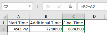
Adding/ Subtracting Time in Excel
So far, we have seen examples where we had the start and the end time, and we needed to find the time difference.
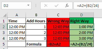
Excel also allows you to easily add or subtract a fixed time value from the existing date and time value.
For example, let’s say you have a list of queued tasks where each task takes the specified time, and you want to know when each task will end.
In such a case, you can easily add the time that each task is going to take to the start time to know at what time is the task expected to be completed.
Since Excel stores date and time values as numbers, you have to ensure that the time you are trying to add abides by the format that Excel already follows.
For example, if you add 1 to a date in Excel, it is going to give you the next date. This is because 1 represents an entire day in Excel (which is equal to 24 hours).
So if you want to add 1 hour to an existing time value, you cannot go ahead and simply add 1 to it. you have to make sure that you convert that hour value into the decimal portion that represents one hour. and the same goes for adding minutes and seconds.
Using the TIME Function
Time function in Excel takes the hour value, the minute value, and the seconds value and converts it into a decimal number that represents this time.
For example, if I want to add 4 hours to an existing time, I can use the below formula:
=Start Time + TIME(4,0,0)

This is useful if you know how many hours, minutes, and seconds you want to add to an existing time and simply use the TIME function without worrying about the correct conversion of the time into a decimal value.
Also, note that the TIME function will only consider the integer part of the hour, minute, and seconds value that you input. For example, if I use 5.5 hours in the TIME function it would only add five hours and ignore the decimal part.
Also, note that the TIME function can only add values that are less than 24 hours. If your hour value is more than 24, this would give you an incorrect result.
And the same goes with the minutes and the second’s part where the function will only consider values that are less than 60 minutes and 60 seconds
Just like I have added time using the TIME function, you can also subtract time. Just change the + sign to a negative sign in the above formulas
Using Basic Arithmetic
When the time function is easy and convenient to use, it does come with a few restrictions (as covered above).
If you want more control, you can use the arithmetic method that I’ll cover here.
The concept is simple – convert the time value into a decimal value that represents the portion of the day, and then you can add it to any time value in Excel.
For example, if you want to add 24 hours to an existing time value, you can use the below formula:
=Start_time + 24/24
This just means that I’m adding one day to the existing time value.
Now taking the same concept forward let’s say you want to add 30 hours to a time value, you can use the below formula:
=Start_time + 30/24
The above formula does the same thing, where the integer part of the (30/24) would represent the total number of days in the time that you want to add, and the decimal part would represent the hours/minutes/seconds
Similarly, if you have a specific number of minutes that you want to add to a time value then you can use the below formula:
=Start_time + (Minutes to Add)/24*60
And if you have the number of seconds that you want to add, then you can use the below formula:
=Start_time + (Minutes to Add)/24*60*60
While this method is not as easy as using the time function, I find it a lot better because it works in all situations and follows the same concept. unlike the time function, you don’t have to worry about whether the time that you want to add is less than 24 hours or more than 24 hours
You can follow the same concept while subtracting time as well. Just change the + to a negative sign in the formulas above
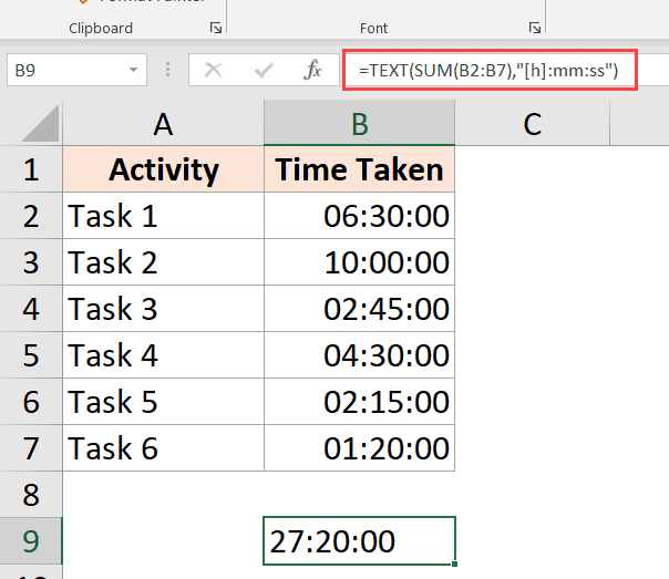
How to SUM time in Excel
Sometimes you may want to quickly add up all the time values in Excel. Adding multiple time values in Excel is quite straightforward (all it takes is a simple SUM formula)
But there are a few things you need to know when you add time in Excel, specifically the cell format that is going to show you the result.
Let’s have a look at an example.
Below I have a list of tasks along with the time each task will take in column B, and I want to quickly add these times and know the total time it is going to take for all these tasks.

In cell B9, I have used a simple SUM formula to calculate the total time all these tasks are going to take, and it gives me the value as 18:30 (which means that it is going to take 18 hours and 20 minutes to complete all these tasks)

All good so far!
How to SUM over 24 hours in Excel
Now see what happens when I change at the time it is going to take Task 2 to complete from 1 hour to 10 hours.

The result now says 03:20, which means that it should take 3 hours and 20 minutes to complete all these tasks.
This is incorrect (obviously)
The problem here is not Excel messing up. The problem here is that the cell is formatted in such a way that it will only show you the time portion of the resulting value.
And since the resulting value here is more than 24 hours, Excel decided to convert the 24 hours part into a day remove it from the value that is shown to the user, and only display the remaining hours, minutes, and seconds.
This, thankfully, has an easy fix.
All you need to do is change the cell format to force it to show hours even if it exceeds 24 hours.
Below are some formats that you can use:
| Format | Expected Result |
| [h]:mm | 28:30 |
| [m]:ss | 1710:00 |
| d “D” hh:mm | 1 D 04:30 |
| d “D” hh “Min” ss “Sec” | 1 D 04 Min 00 Sec |
| d “Day” hh “Minute” ss “Seconds” | 1 Day 04 Minute 00 Seconds |
You can change the format by going to the format cells dialog box and applying the custom format, or use the TEXT function and use any of the above formats in the formula itself
You can use the below the TEXT formula to show the time, even when it’s more than 24 hours:
=TEXT(SUM(B2:B7),"[h]:mm:ss")
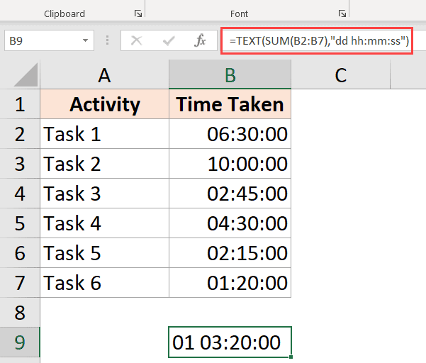
or the below formula if you want to convert the hours exceeding 24 hours to days:
=TEXT(SUM(B2:B7),"dd hh:mm:ss")
Results Showing Hash (###) Instead of Date/Time (Reasons + Fix)
In some cases, you may find that instead of showing you the time value, Excel is displaying the hash symbols in the cell.
Here are some possible reasons and the ways to fix these:
The column is not wide enough
When a cell doesn’t have enough space to show the complete date, it may show the hash symbols.
It has an easy fix – change the column width and make it wider.
Negative Date Value
A date or time value cannot be negative in Excel. in case you are calculating the time difference and it turns out to be negative, Excel will show you hash symbols.
The way to fixes to change the formula to give you the right result. For example, if you are calculating the time difference between the two times, and the date changes, you need to adjust the formula to account for it.
In other cases, you may use the ABS function to convert the negative time value into a positive number so that it’s displayed correctly. Alternatively, you can also an IF formula to check if the result is a negative value and return something more meaningful.
In this tutorial, I covered topics about calculating time in Excel (where you can calculate the time difference, add or subtract time, show time in different formats, and sum time values)
I hope you found this tutorial useful.
Other Excel tutorials you may also like:
- Convert Time to Decimal Number in Excel (Hours, Minutes, Seconds)
- How to Remove Time from Date/Timestamp in Excel
- How to Calculate the Number of Days Between Two Dates in Excel
- Combine Date and Time in Excel
- How to Calculate Years of Service in Excel
- How to Convert Seconds to Minutes in Excel
Purpose
Create a time with hours, minutes, and seconds
Return value
A decimal number representing a particular time in Excel.
Usage notes
The TIME function creates a valid Excel time based with supplied values for hour, minute, and second. Like all Excel time, the result is a number that represents a fractional day. The TIME function will only return time values up to one full day, between 0 (zero) to 0.99999999, or 0:00:00 to 23:59:59. To see results formatted as time, apply a time-based number format.
Examples
=TIME(3,0,0) // 3 hours
=TIME(0,3,0) // 3 minutes
=TIME(0,0,3) // 3 seconds
=TIME(8,30,0) // 8.5 hours
The TIME function can interpret units in larger increments. For example, both of the formulas below return a result of 2 hours:
=TIME(0,120,0) // 2 hours
=TIME(0,0,7200) // 2 hours
However, when total time reaches 24 hours, the TIME function will «reset» to zero.
=TIME(12,0,0) // 12 hours
=TIME(36) // 12 hours
In this way, TIME behaves like a 24 hour clock that resets when it crosses midnight. Notably, TIME will not handle numeric inputs larger 32,767. For example, even though there are 86,400 seconds in a day, the following formula (which represents 12 hours) will fail with a #NUM! error:
=TIME(0,0,43200) // returns #NUM!
As a workaround, you can convert hours, minutes, and seconds directly to Excel time with a formula:
=hours/24+minutes/1440+seconds/86400
The result is the same as the TIME function up to 24 hours. Over 24 hours, this formula will continue to accumulate time, unlike the TIME function.
Notes
- When total time reaches 24 hours, the TIME function will «reset» to zero.
- The largest number that TIME will allow for hour, minute, or second is 32,767. Larger values will return a #NUM! error.
Date and time in excel are treated a bit differently in excel than in other spreadsheets software. If you don’t know how Excel date and time work, you may face unnecessary errors.
So, in this article, we will learn everything about the date and time of Excel. We will learn, what are dates in excel, how to add time in excel, how to format date and time in excel, what are date and time functions in excel, how to do date and time calculations (adding, subtracting, multiplying etc. with dates and times).
What is Date and Time in Excel?
Many of you may already know that Excel dates and time are nothing but serial numbers. A date is a whole number and time is a fractional number. Dates in excel have different regional formatting. For example, in my system, it is mm/dd/YYYY (we will use this format throughout the article). You may be using the same date format or you could be using dd/mm/YYYY date format.
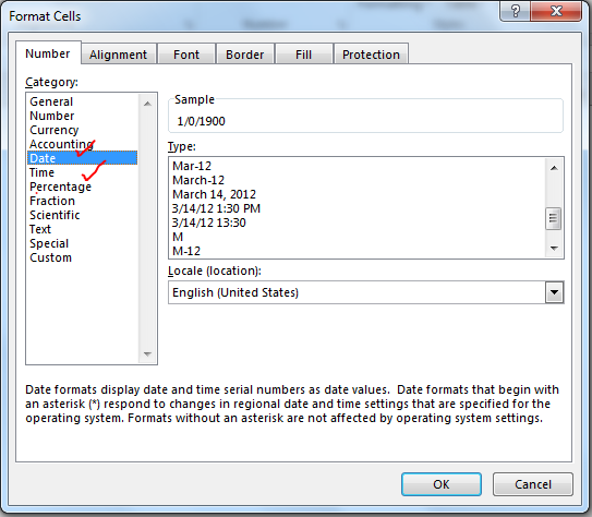
Date Formatting of Cell
There are multiple options available to format a date in Excel. Select a cell that may contain a date and press CTRL+1. This will open the Format Cells dialogue box. Here you can see two formatting options as Date and Time. In these categories, there are multiple date formattings available to suit your requirements.
 Dates:
Dates in Excel are mare serial numbers starting from 1-Jan-1900. A day in excel is equal to 1. Hence 1-Jan-1900 is 1, 2-Jan-1900 is 2, and 1-Jan-2000 is 36526.
Fun Fact: 1900 was not a leap year but excel accepts 29-Feb-1900 as a valid date. It was a desperate glitch to compete Lotus 1-2-3 back in those days.
Shortcut to enter static today’s date in excel is CTRL+; (Semicolon).
To add or subtract a day from a date you just need to subtract or add that number of days to that date.
Time:
Excel by default follows the hh:mm format for time (0 to 23 format). The hours and minutes are separated by a colon without any spaces in between. You can change it to hh:mm AM/PM format. The AM/PM must have 1 space from the time value. To include seconds, you can add :ss to hh:mm (hh:mm:ss). Any other time format is invalid.
Time is always associated with a date. The date comes before the time value separated with a space from time. If you don’t mention a date before time, by default it takes the first date of excel (which is 1/1/1900). Time in excel is a fractional number. It is shown on the right side of the decimal.
Hours:
Since 1 day is equal to 1 in excel and 1 day consists of 24 hours, 1 hour is equal to 1/24 in excel. What does that mean? It means that if you want to add or subtract 1 hour to time, you need to add or subtract 1/24. See the image below.
 you can say that 1 hour is equal to 0.041666667 (1/24).
Calculate hours between time in Excel
Minutes:
From the explanation of the hour in excel, you must have guessed that 1 Minute in excel is equal to 1/(24×60) (or 1/1440 or 0.000694444).
If you want to add a minute to an excel time, add 1/(24×60). See the image below. Sometimes you get the need to Calculate Minutes Between Dates & Time In Excel, you can read it here.
 Seconds:
Yes, a second in Excel is equal to 1/(24x60x60). To add or subtract seconds from a time, you just need to do the same things as we did in minutes and hours.
Date and Time in one cell
Dates and times are linked together. A date is always associated with a valid date and time is always associated with a valid excel date. Even if you are not able to see one of them.
If you only enter a time in a cell, the date of that cell will 1-Jan-1900, even if you are not able to see it. If you format that cell as a date-time format, you can see the associated date. Similarly, if you don’t mention time with the date, by default 12:00 AM is attached. See the image below.
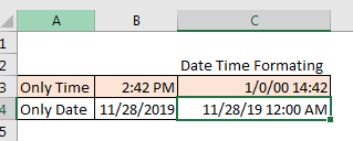
In the image above, we have time only in B3 and date only in B4. When we format these cells as mm/dd/yy hh:mm, we get both, time and date in both cells.
So, while doing date and time calculations in excel, keep this in check.
No Negative Time
As I told you the date and time in excel starts from 1-Jan-1900 12:00 AM. Any time before this is not a valid date in excel. If you subtract a value from a date that leads to before 1-Jan-1900 12:00, even one second, excel will produce ###### error. I have talked about it here and in Convert Date and Time from GMT to CST. It happens when we try to subtract something that leads to before 1 Jan-1900 12:00. Try it yourself. Write 12:00 PM and subtract 13 hours from it. see what you get.
Calculations with Dates and Time in Excel
Adding Days to a date:
Adding days to a date in excel is easy. To add a day to date just add 1 to it. See the image below.
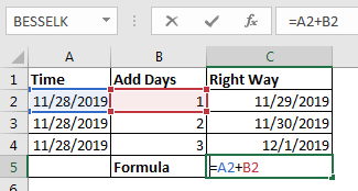
You should not add two dates to get the future date, as it will sum up the serial numbers of those days and you may get a date far in the future.
Subtracting Days from Date:
If you want to get a backdate from a date a few days before, then just subtract that number of days from the date and you will get backdate. For example, if I want to know what date was before 56 days since TODAY then I would write this formula in the cell.
This will return us the date of 56 before the current date.
Note: Remember that you can not have a date before 1/Jan/1900 in excel. If you get ###### error, this could be the reason.
Days between two dates:
To calculate days between two dates we just need to subtract the start date from the end date. I have already done an article on this topic. Go and check it out here. You can also use the Excel DAYS Function to calculate days between a start date and end date.
Adding Times:
There’s been a lot of queries on how to add time to excel as many people get confusing results when they do it. There are two types of addition in times. One is adding time to another time. In this case, both times are formatted as hh:mm time format. In this case, you can simply add these times.
The second case is when you don’t have additional time in time format. You just have numbers of hours, minutes and seconds to add. In that case, you need to convert those numbers to their time equivalents. Note these points to add hours, minutes and seconds to a date/time.
- To add N hours to an X time use formula =X+(N/24) (As 1=24 hours)
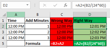
- To Add N minutes to X time use formula = X+(N/(24*60))
- To Add N Second to X time use formula = X+(N/(24*60*60))
Subtracting Times
It’s the same as adding time, just make sure that you don’t end up with a negative time value when subtracting, because there is no such thing as a negative number in excel.
Note: When you add or subtract time in excel that exceeds 24 hours of difference, excel will roll to the next or previous date. For example, if you subtract 2 hours from 29-Jan-2019 1:00 AM then it will roll back to 28-Jan-2019 11:00 PM. If you subtract 2 hours from 1:00 AM (does not have the date mentioned), Excel will return ###### error. I have told the reason at the beginning of the article.
Adding Months to a Date:
You can’t just add multiples of 30 to add months to date as different months have a different number of days. You need to be careful while adding months to Date. To add months to a date in excel, we use EDATE function of excel. Here I have a separate article on adding months to a date in different scenarios.
 Adding years to date:
Just like adding months to a date, it is not straightforward to add years to date. We need to use YEAR, MONTH, DAY function to add years to date. You can read about adding years to date here.
If you want to calculate years between dates then you can use this.
Excel Date and Time Handling Functions:
Since date and time are special in Excel, Excel provides special functions to handle them. Here I am mentioning a few of them.
- TODAY(): This function returns today’s date dynamically.
- DAY(): Returns Day of the month (returns number 1 to 31).
- DAYS(): Used to count the number of days between two dates.
- MONTH(): Used to get the month of the date (returns number 1 to 12).
- YEAR(): Returns year of the date.
- WEEKNUM(): Returns the weekly number of a date, in a year.
- WEEKDAY(): Returns the day number in a week (1 to 7) of the supplied date.
- WORKDAY(): Used to calculate working days.
- TIMEVALUE(): Used to extract Time value (serial number) from a text formatted date and time.
- DATEVALUE(): Used to extract date value (serial number) from a text formatted date and time.
These are some of the most useful data and time functions in excel. There are plenty more date and time functions. You can check them out here.
Date and Time Calculations
If I explain all of them here, this article will get too long. I have divided these time calculation techniques in excel into separate articles. Here I am mentioning them. You can click on them to read.
- Calculate days, months and years
- Calculate age from date of birth
- Multiplying time values and numbers.
- Get Month name from Date in Excel
- Get day name from Date in Excel
- How to get a quarter of the year from date
- How to Add Business Days in Excel
- Insert Date Time Stamp with VBA
So yeah guys, this is all about the date and time in excel you need to know about. I hope this article was useful to you. If you have any queries or suggestions, write them down in the comments section below.
Excel defaults to date and time functions: HOUR, MINUTE and SECOND. Consider in detail these three functions in action on specific examples. How, when and where they can be effectively applied, making up various formulas from these functions for working with time.
Examples of using the functions HOUR, MINUTE and SECOND for calculations in Excel
The HOUR function in Excel is designed to determine the hour value from the transmitted time as a parameter and returns data from a range of numeric values from 0 to 23, depending on the format of the temporary record.
The function MINUTE in Excel is used to get the minutes from the transmitted data, which characterizes the time, and returns data from a range of numeric values from 0 to 59.
The SECOND function in Excel is used to get the seconds from data in a time format and returns numeric values from 0 to 59.
Monitoring the daily time clock in Excel using the HOUR function
Example 1. Get the current time, determine how many hours have passed since the beginning of the current day, how many hours left before the beginning of a new day.
Source table:
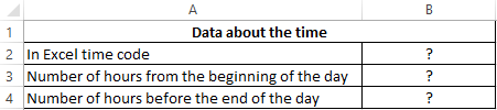
Let’s define the current moment in the Excel time code:
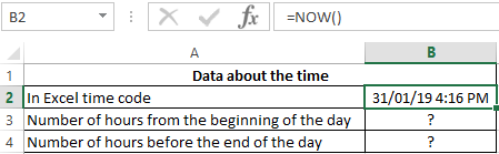
Calculate the number of hours from the beginning of the day:
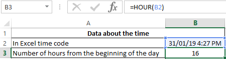
- B2 — the current date and time, expressed in the format Date.
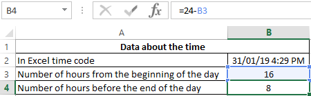
Determine the number of hours before the end of the day:
Argument Description:
- 24 — the number of hours per day;
- B3 is the current time in hours, expressed as a numerical value.
Note: The example demonstrates that the result of the work of the HOUR function is a number on which you can perform any arithmetic operation.
Conversion of numbers to time format using the functions HOUR and MINUTE
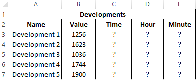
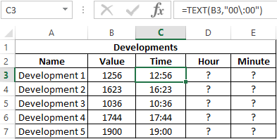
Example 2. From the application, moments of passing certain events that were recognized by Excel as ordinary numbers were loaded (for example, 13:05 was recognized as the number 1305). It is necessary to convert the obtained values into the time format, select the hours and minutes.
Source data table:
To convert the data, use the function:
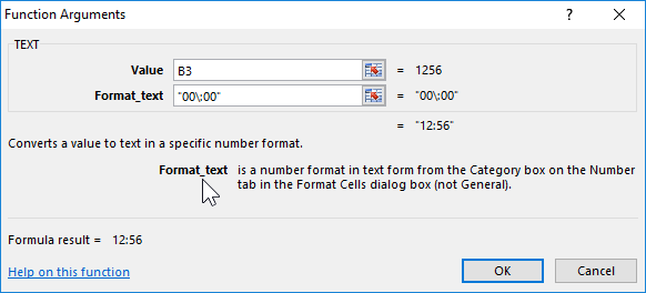
=TEXT(B3,»00:00″)
Argument Description:
- B3 — the value recognized by Excel as a normal number;
- «00:00» is the time format.
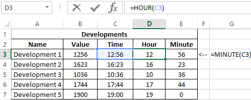
As a result, we get:
Using the functions HOUR and MINUTE, select the desired values. Similarly, we define the required values for the remaining events:
Example of using the SECOND function in Excel
Example 3. The work day starts at 8:00 am. One worker was systematically late for the previous 10 working days for a few seconds. Determine the total time the employee is late.
Enter the data in the table:
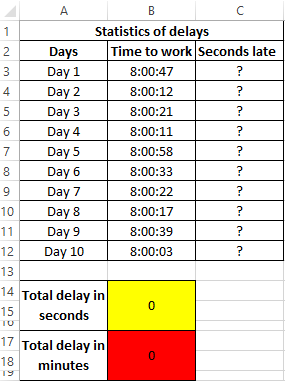
Determine the delay in seconds. Where B3 — data on the time of arrival at work on the first day. Similarly, we define the seconds of delay for the following days:
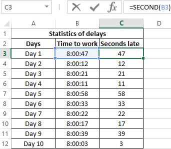
Determine the total number of seconds of delay:
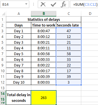
Where C3:C12 is an array of cells containing seconds of late values. We define the integer value of the minutes of delay, knowing that in 1 min = 60 seconds. As a result, we get:
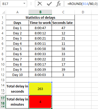
That is, the total lateness of an employee for 10 days was 263 seconds, which is more than 4 minutes.
Features syntax functions HOUR, MINUTE and SECOND in Excel
The HOUR function has the following syntax entry:
=HOUR(serial_number)
- serial_number is the only function argument (required) that characterizes time data that contains data about the clock.
Notes:
- If a string with text that does not contain time information is passed as an argument to the HOUR function, the error code #VAL! Will be returned.
- If the logical data type (TRUE, FALSE) or a reference to an empty cell was passed as an argument to the HOUR function, the value 0 will be returned.
- There are several permitted data formats that the HOUR function accepts:
- In Excel time code (range of values from 0 to 2958465), while the integers correspond to days, fractional — hours, minutes and seconds. For example, 43284.5 is the number of days elapsed between the current moment and the starting point of reference in Excel (01/01/1900 is a conditional date). Fractional part 0.5 corresponds to 12 hours (half of the day).
- In the form of a text string, for example =HOUR(“11:57”). The result of the function — the number 11.
- In the format of the Date and Time Excel. For example, the function will return the values of the clock if, as an argument, it receives a reference to the cell containing the value “07/03/18 11:24” in the date format.
- As a result of the function that returns data in a time format. For example, the function =HOUR(TIMEVALUE(“1:34”)) returns the value 1.
The MINUTE function has the following syntax:
=MINUTE(serial_number)
- serial_number is a required argument describing the value from which the minutes will be calculated.
Notes:
- As in the case of the HOUR function, the MINUTE function accepts text and numeric data in the format of Dates and Times.
- If the argument of this function is an empty text string (“”) or a string containing text (“some text”), the error #VALUE! Will be returned.
- The function supports date format in Excel time code (for example, =MINUTE(0.34) returns the value 9).
The syntax of the SECOND function in Excel is:
=SECOND(serial_number)
- serial_number is the only argument represented as data from which the seconds will be calculated (required for filling).
Download examples HOUR, MINUTE and SECOND to work with time in Excel
Notes:
- The SECOND function works with text and numeric data types representing Date and Time in Excel.
- Error #VALUE! will occur in cases where the argument is a text string that does not contain data characterizing the time.
- The function also calculates seconds from the number represented in the Excel time code (for example, =SECOND(9,567) returns the value 29).
Содержание
- Работа с функциями даты и времени
- ДАТА
- РАЗНДАТ
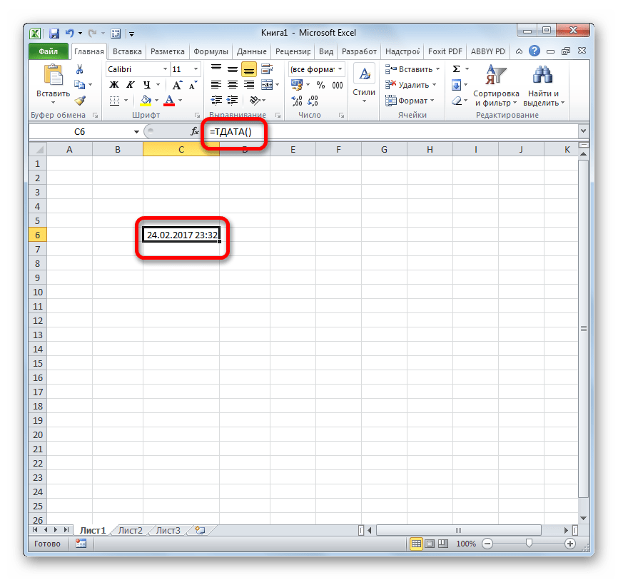
- ТДАТА
- СЕГОДНЯ
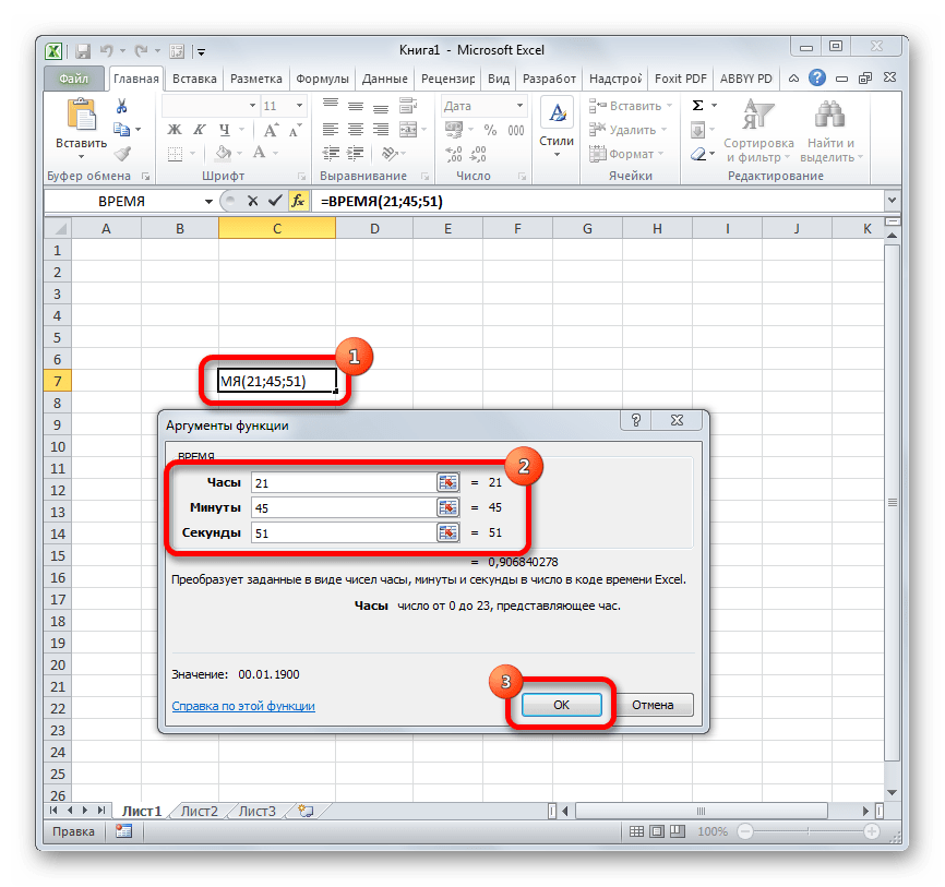
- ВРЕМЯ
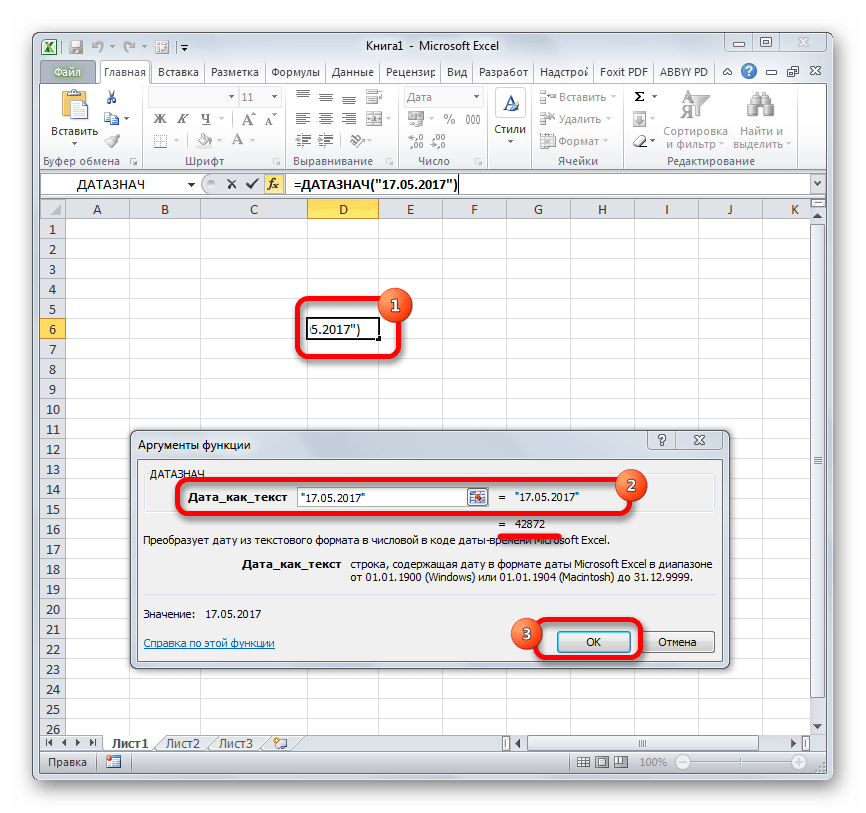
- ДАТАЗНАЧ
- ДЕНЬНЕД
- НОМНЕДЕЛИ
- ДОЛЯГОДА
- Вопросы и ответы
Одной из самых востребованных групп операторов при работе с таблицами Excel являются функции даты и времени. Именно с их помощью можно проводить различные манипуляции с временными данными. Дата и время зачастую проставляется при оформлении различных журналов событий в Экселе. Проводить обработку таких данных – это главная задача вышеуказанных операторов. Давайте разберемся, где можно найти эту группу функций в интерфейсе программы, и как работать с самыми востребованными формулами данного блока.
Работа с функциями даты и времени
Группа функций даты и времени отвечает за обработку данных, представленных в формате даты или времени. В настоящее время в Excel насчитывается более 20 операторов, которые входят в данный блок формул. С выходом новых версий Excel их численность постоянно увеличивается.
Любую функцию можно ввести вручную, если знать её синтаксис, но для большинства пользователей, особенно неопытных или с уровнем знаний не выше среднего, намного проще вводить команды через графическую оболочку, представленную Мастером функций с последующим перемещением в окно аргументов.
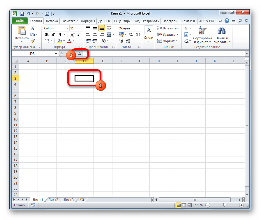
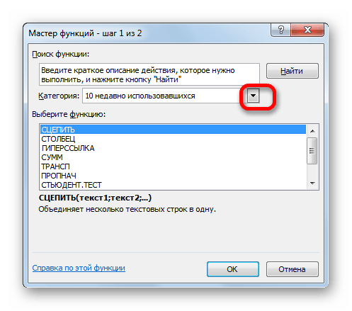
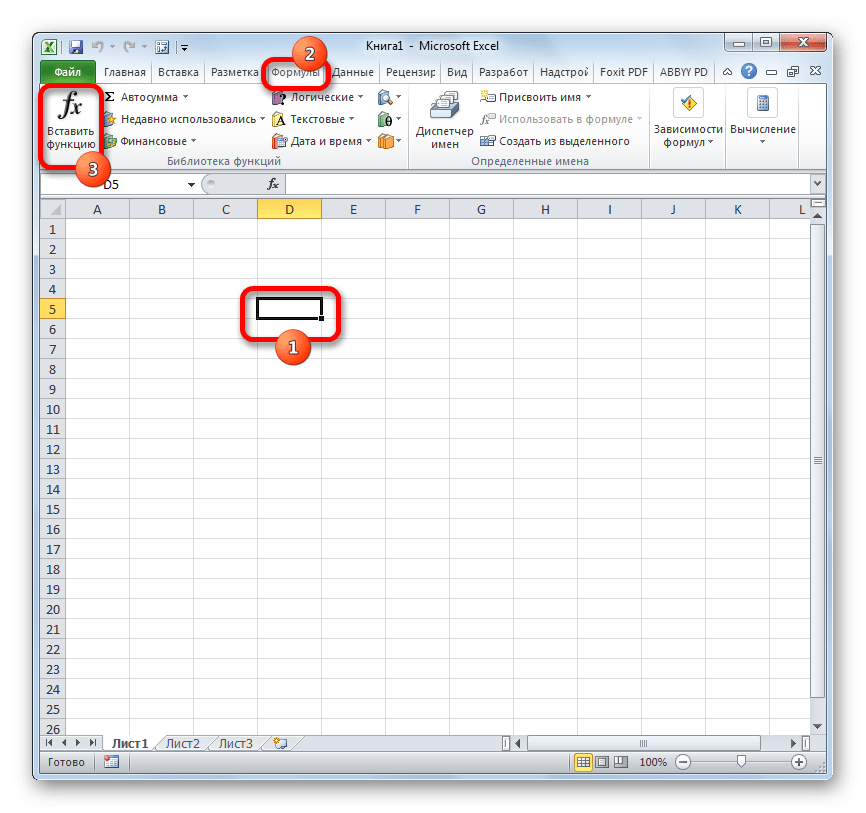
- Для введения формулы через Мастер функций выделите ячейку, где будет выводиться результат, а затем сделайте щелчок по кнопке «Вставить функцию». Расположена она слева от строки формул.
- После этого происходит активация Мастера функций. Делаем клик по полю «Категория».
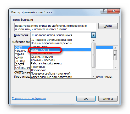
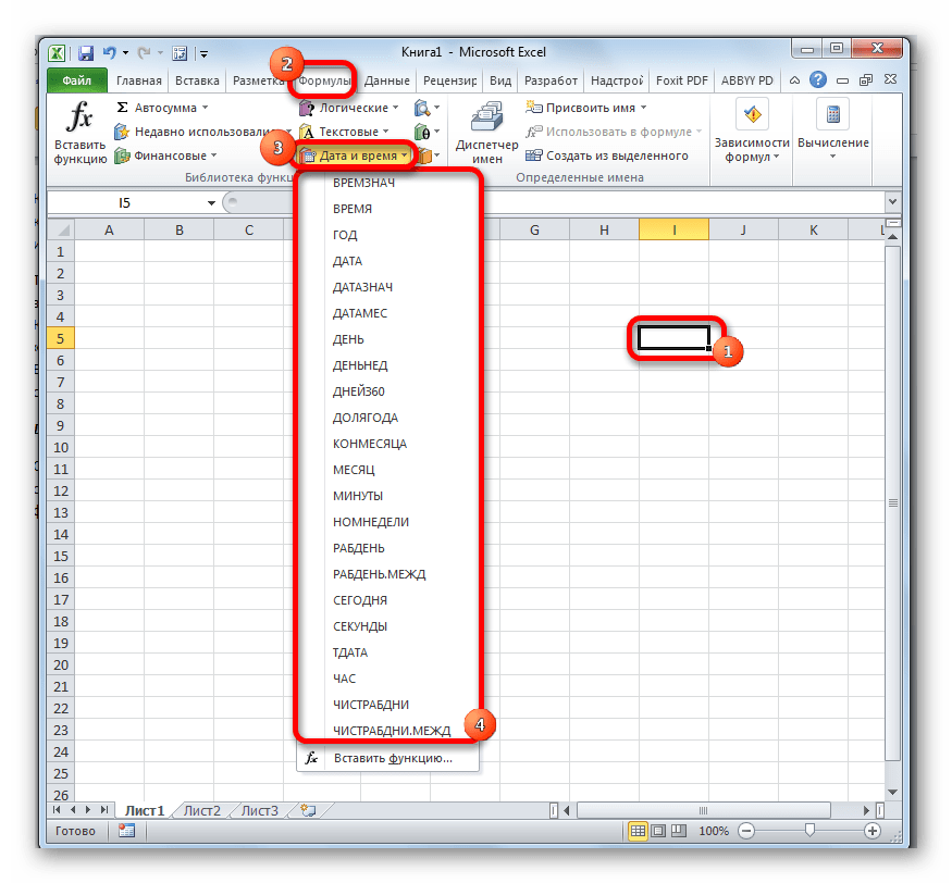
- Из открывшегося списка выбираем пункт «Дата и время».
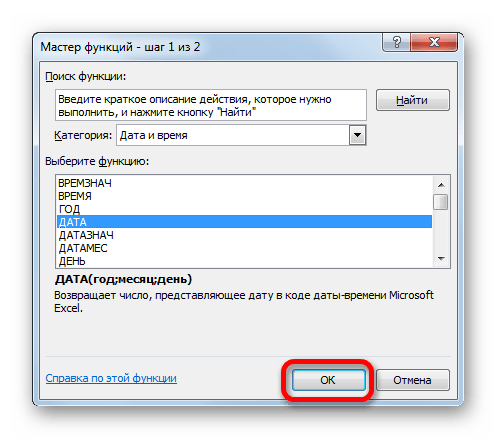
- После этого открывается перечень операторов данной группы. Чтобы перейти к конкретному из них, выделяем нужную функцию в списке и жмем на кнопку «OK». После выполнения перечисленных действий будет запущено окно аргументов.
Кроме того, Мастер функций можно активировать, выделив ячейку на листе и нажав комбинацию клавиш Shift+F3. Существует ещё возможность перехода во вкладку «Формулы», где на ленте в группе настроек инструментов «Библиотека функций» следует щелкнуть по кнопке «Вставить функцию».
Имеется возможность перемещения к окну аргументов конкретной формулы из группы «Дата и время» без активации главного окна Мастера функций. Для этого выполняем перемещение во вкладку «Формулы». Щёлкаем по кнопке «Дата и время». Она размещена на ленте в группе инструментов «Библиотека функций». Активируется список доступных операторов в данной категории. Выбираем тот, который нужен для выполнения поставленной задачи. После этого происходит перемещение в окно аргументов.
Урок: Мастер функций в Excel
ДАТА
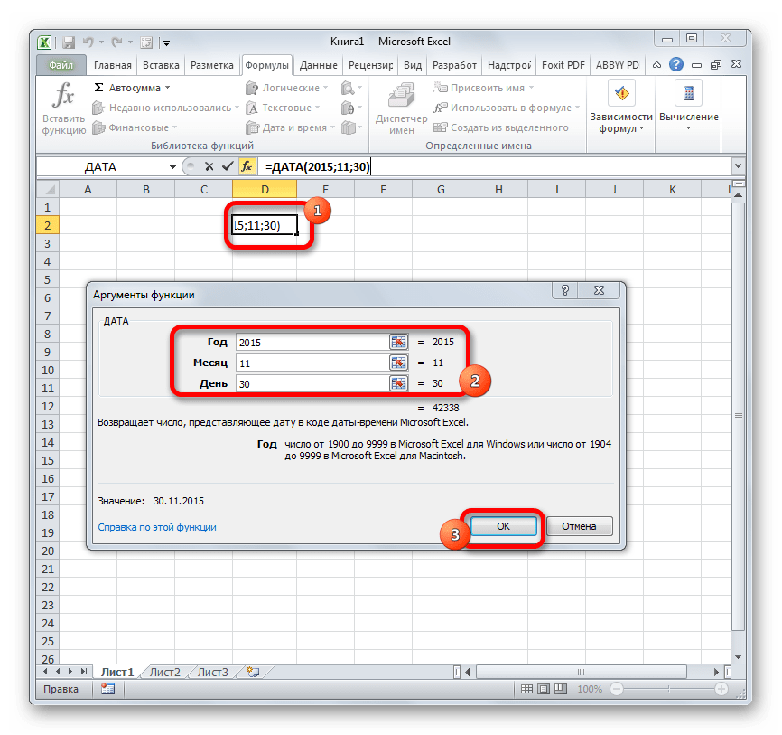
Одной из самых простых, но вместе с тем востребованных функций данной группы является оператор ДАТА. Он выводит заданную дату в числовом виде в ячейку, где размещается сама формула.
Его аргументами являются «Год», «Месяц» и «День». Особенностью обработки данных является то, что функция работает только с временным отрезком не ранее 1900 года. Поэтому, если в качестве аргумента в поле «Год» задать, например, 1898 год, то оператор выведет в ячейку некорректное значение. Естественно, что в качестве аргументов «Месяц» и «День» выступают числа соответственно от 1 до 12 и от 1 до 31. В качестве аргументов могут выступать и ссылки на ячейки, где содержатся соответствующие данные.

Для ручного ввода формулы используется следующий синтаксис:
=ДАТА(Год;Месяц;День)
Близки к этой функции по значению операторы ГОД, МЕСЯЦ и ДЕНЬ. Они выводят в ячейку значение соответствующее своему названию и имеют единственный одноименный аргумент.
РАЗНДАТ
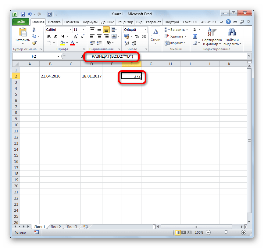
Своего рода уникальной функцией является оператор РАЗНДАТ. Он вычисляет разность между двумя датами. Его особенность состоит в том, что этого оператора нет в перечне формул Мастера функций, а значит, его значения всегда приходится вводить не через графический интерфейс, а вручную, придерживаясь следующего синтаксиса:
=РАЗНДАТ(нач_дата;кон_дата;единица)
Из контекста понятно, что в качестве аргументов «Начальная дата» и «Конечная дата» выступают даты, разницу между которыми нужно вычислить. А вот в качестве аргумента «Единица» выступает конкретная единица измерения этой разности:
- Год (y);
- Месяц (m);
- День (d);
- Разница в месяцах (YM);
- Разница в днях без учета годов (YD);
- Разница в днях без учета месяцев и годов (MD).
Урок: Количество дней между датами в Excel
ЧИСТРАБДНИ
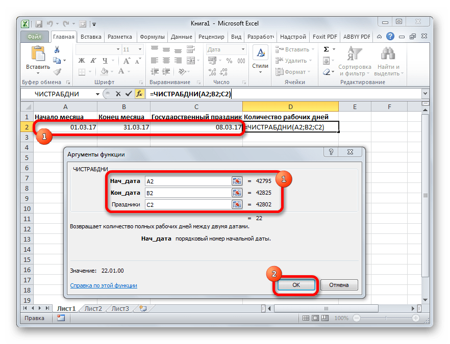
В отличии от предыдущего оператора, формула ЧИСТРАБДНИ представлена в списке Мастера функций. Её задачей является подсчет количества рабочих дней между двумя датами, которые заданы как аргументы. Кроме того, имеется ещё один аргумент – «Праздники». Этот аргумент является необязательным. Он указывает количество праздничных дней за исследуемый период. Эти дни также вычитаются из общего расчета. Формула рассчитывает количество всех дней между двумя датами, кроме субботы, воскресенья и тех дней, которые указаны пользователем как праздничные. В качестве аргументов могут выступать, как непосредственно даты, так и ссылки на ячейки, в которых они содержатся.
Синтаксис выглядит таким образом:
=ЧИСТРАБДНИ(нач_дата;кон_дата;[праздники])
ТДАТА
Оператор ТДАТА интересен тем, что не имеет аргументов. Он в ячейку выводит текущую дату и время, установленные на компьютере. Нужно отметить, что это значение не будет обновляться автоматически. Оно останется фиксированным на момент создания функции до момента её перерасчета. Для перерасчета достаточно выделить ячейку, содержащую функцию, установить курсор в строке формул и кликнуть по кнопке Enter на клавиатуре. Кроме того, периодический пересчет документа можно включить в его настройках. Синтаксис ТДАТА такой:
=ТДАТА()
СЕГОДНЯ
Очень похож на предыдущую функцию по своим возможностям оператор СЕГОДНЯ. Он также не имеет аргументов. Но в ячейку выводит не снимок даты и времени, а только одну текущую дату. Синтаксис тоже очень простой:
=СЕГОДНЯ()
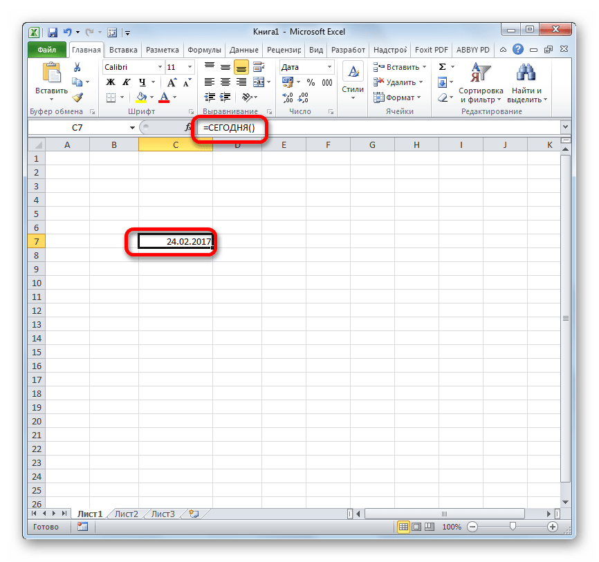
Эта функция, так же, как и предыдущая, для актуализации требует пересчета. Перерасчет выполняется точно таким же образом.
ВРЕМЯ
Основной задачей функции ВРЕМЯ является вывод в заданную ячейку указанного посредством аргументов времени. Аргументами этой функции являются часы, минуты и секунды. Они могут быть заданы, как в виде числовых значений, так и в виде ссылок, указывающих на ячейки, в которых хранятся эти значения. Эта функция очень похожа на оператор ДАТА, только в отличии от него выводит заданные показатели времени. Величина аргумента «Часы» может задаваться в диапазоне от 0 до 23, а аргументов минуты и секунды – от 0 до 59. Синтаксис такой:
=ВРЕМЯ(Часы;Минуты;Секунды)
Кроме того, близкими к этому оператору можно назвать отдельные функции ЧАС, МИНУТЫ и СЕКУНДЫ. Они выводят на экран величину соответствующего названию показателя времени, который задается единственным одноименным аргументом.
ДАТАЗНАЧ
Функция ДАТАЗНАЧ очень специфическая. Она предназначена не для людей, а для программы. Её задачей является преобразование записи даты в обычном виде в единое числовое выражение, доступное для вычислений в Excel. Единственным аргументом данной функции выступает дата как текст. Причем, как и в случае с аргументом ДАТА, корректно обрабатываются только значения после 1900 года. Синтаксис имеет такой вид:
=ДАТАЗНАЧ (дата_как_текст)
ДЕНЬНЕД
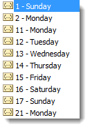
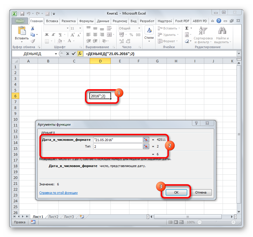
Задача оператора ДЕНЬНЕД – выводить в указанную ячейку значение дня недели для заданной даты. Но формула выводит не текстовое название дня, а его порядковый номер. Причем точка отсчета первого дня недели задается в поле «Тип». Так, если задать в этом поле значение «1», то первым днем недели будет считаться воскресенье, если «2» — понедельник и т.д. Но это не обязательный аргумент, в случае, если поле не заполнено, то считается, что отсчет идет от воскресенья. Вторым аргументом является собственно дата в числовом формате, порядковый номер дня которой нужно установить. Синтаксис выглядит так:
=ДЕНЬНЕД(Дата_в_числовом_формате;[Тип])
НОМНЕДЕЛИ
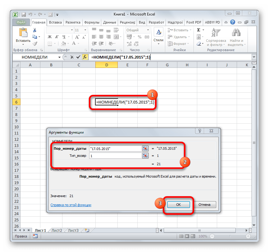
Предназначением оператора НОМНЕДЕЛИ является указание в заданной ячейке номера недели по вводной дате. Аргументами является собственно дата и тип возвращаемого значения. Если с первым аргументом все понятно, то второй требует дополнительного пояснения. Дело в том, что во многих странах Европы по стандартам ISO 8601 первой неделей года считается та неделя, на которую приходится первый четверг. Если вы хотите применить данную систему отсчета, то в поле типа нужно поставить цифру «2». Если же вам более по душе привычная система отсчета, где первой неделей года считается та, на которую приходится 1 января, то нужно поставить цифру «1» либо оставить поле незаполненным. Синтаксис у функции такой:
=НОМНЕДЕЛИ(дата;[тип])
ДОЛЯГОДА
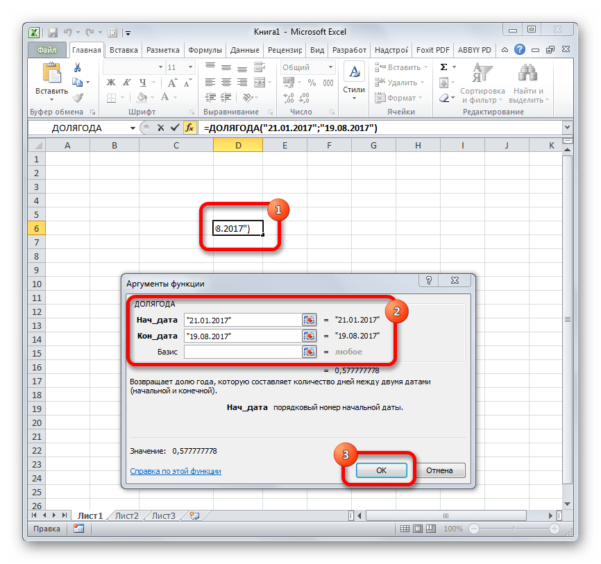
Оператор ДОЛЯГОДА производит долевой расчет отрезка года, заключенного между двумя датами ко всему году. Аргументами данной функции являются эти две даты, являющиеся границами периода. Кроме того, у данной функции имеется необязательный аргумент «Базис». В нем указывается способ вычисления дня. По умолчанию, если никакое значение не задано, берется американский способ расчета. В большинстве случаев он как раз и подходит, так что чаще всего этот аргумент заполнять вообще не нужно. Синтаксис принимает такой вид:
=ДОЛЯГОДА(нач_дата;кон_дата;[базис])
Мы прошлись только по основным операторам, составляющим группу функций «Дата и время» в Экселе. Кроме того, существует ещё более десятка других операторов этой же группы. Как видим, даже описанные нами функции способны в значительной мере облегчить пользователям работу со значениями таких форматов, как дата и время. Данные элементы позволяют автоматизировать некоторые расчеты. Например, по введению текущей даты или времени в указанную ячейку. Без овладения управлением данными функциями нельзя говорить о хорошем знании программы Excel.
Skip to content
В статье рассматривается, как в Excel посчитать время. Вы найдете несколько полезных формул чтобы посчитать сумму времени, разницу во времени или сколько времени прошло и многое другое.
Ранее мы внимательно рассмотрели особенности формата времени Excel и возможности основных функций времени. Сегодня мы углубимся в вычисления времени в Excel, и вы узнаете еще несколько формул для эффективного управления временем в ваших таблицах.
Как посчитать разницу во времени в Excel (прошедшее время)
Для начала давайте посмотрим, как можно быстро посчитать в Excel сколько прошло времени, т.е. найти разницу между временем начала и временем окончания. И, как это часто бывает, существует несколько способов для расчета времени. Какую из них выбрать, зависит от вашего набора данных и того, какого именно результата вы пытаетесь достичь. Итак, давайте посмотрим несколько вариантов.
Вычесть одно время из другого
Как вы, наверное, знаете, время в Excel — это обычные десятичные числа, отформатированные так, чтобы они выглядели как время. И поскольку это числа, вы можете складывать и вычитать время так же, как и любые другие числовые значения.
Самая простая и очевидная формула Excel чтобы посчитать время от одного момента до другого:
= Время окончания — Время начала
В зависимости от ваших данных, формула разницы во времени может принимать различные формы, например:
| Формула | Пояснение |
| =A2-B2 | Вычисляет разницу между временами в ячейках A2 и B2. |
| =ВРЕМЗНАЧ(«21:30») — ВРЕМЗНАЧ («8:40») | Вычисляет разницу между указанными моментами времени, которые записаны как текст. |
| =ВРЕМЯ(ЧАС(A2); МИНУТЫ(A2); СЕКУНДЫ(A2)) — ВРЕМЯ (ЧАС (B2); МИНУТЫ (B2); СЕКУНДЫ (B2)) | Вычисляет разницу во времени между значениями в ячейках A2 и B2, игнорируя разницу в датах, когда ячейки содержат значения даты и времени. |
Помня, что во внутренней системе Excel время представлено дробной частью десятичного числа, вы, скорее всего, получите результаты, подобные этому скриншоту:

В зависимости оп применяемого форматирования, в столбце D вы можете увидеть десятичные дроби (если установлен формат Общий). Чтобы сделать результаты более информативными, вы можете настроить отображаемый формат времени с помощью одного из следующих шаблонов:
| Формат | Объяснение |
| ч | Прошедшее время отображается только в часах, например: 4. |
| ч:мм | Прошедшие часы и минуты отображаются в формате 4:50. |
| ч:мм:сс | Прошедшие часы, минуты и секунды отображаются в формате 4:50:15. |
Чтобы применить пользовательский формат времени, используйте комбинацию клавиш Ctrl + 1, чтобы открыть диалоговое окно «Формат ячеек», выберите «Пользовательский» и введите шаблон формата в поле «Тип». Подробные инструкции вы можете найти в статье Создание пользовательского формата времени в Excel .
А теперь давайте разберем это на простых примерах. Если время начала находится в столбце B, а время окончания — в столбце A, вы можете использовать эту простую формулу:
=$A2-$B2
Прошедшее время отображается по-разному в зависимости от использованного формата времени, как видно на этом скриншоте:

Примечание. Если время отображается в виде решеток (#####), то либо ячейка с формулой недостаточно широка, чтобы вместить полученный результат, либо итогом ваших расчетов времени является отрицательное число. Отрицательное время в Экселе недопустимо, но это ограничение можно обойти, о чем мы поговорим далее.
Вычисление разницы во времени с помощью функции ТЕКСТ
Еще один простой метод расчета продолжительности между двумя временами в Excel — применение функции ТЕКСТ:
- Рассчитать часы между двумя временами: =ТЕКСТ(A2-B2; «ч»)
- Рассчитать часы и минуты: =ТЕКСТ(A2-B2;»ч:мм»)
- Посчитать часы, минуты и секунды: =ТЕКСТ(A2-B2;»ч:мм:сс»)
Как видно на скриншоте ниже, вы сразу получаете время в нужном вам формате. Специально устанавливать пользовательский формат ячейки не нужно.

Примечание:
- Значение, возвращаемое функцией ТЕКСТ, всегда является текстом. Обратите внимание на выравнивание по левому краю содержимого столбцов C:E на скриншоте выше. В некоторых случаях это может быть существенным ограничением, поскольку вы не сможете использовать полученное «текстовое время» в других вычислениях.
- Если результатом является отрицательное число, ТЕКСТ возвращает ошибку #ЗНАЧ!.
Как сосчитать часы, минуты или секунды
Чтобы получить разницу во времени только в какой-то одной единице времени (только в часах, минутах или секундах), вы можете выполнить следующие вычисления.
Как рассчитать количество часов.
Чтобы представить разницу в часах между двумя моментами времени в виде десятичного числа, используйте следующую формулу:
=( Время окончания — Время начала ) * 24
Если начальное время записано в A2, а время окончания – в B2, вы можете использовать простое выражение B2-A2, чтобы вычислить разницу между ними, а затем умножить результат на 24. Это даст количество часов:
=(B2-A2)* 24
Чтобы получить количество полных часов, используйте функцию ЦЕЛОЕ, чтобы округлить результат до ближайшего целого числа:
=ЦЕЛОЕ((B2-A2) * 24)
Пример расчета разницы во времени только в одной единице измерения вы видите на скриншоте ниже.

Считаем сколько минут в интервале времени.
Чтобы вычислить количество минут между двумя метками времени, умножьте разницу между ними на 1440, что соответствует количеству минут в одном дне (24 часа * 60 минут = 1440).
=( Время окончания — Время начала ) * 1440
Как показано на скриншоте выше, формула может возвращать как положительные, так и отрицательные значения. Отрицательные возникают, когда время окончания меньше времени начала, как в строке 5:
=(B2-A2)*1440
Как сосчитать количество секунд.
Чтобы посчитать разницу в секундах между двумя моментами времени, вы умножаете разницу во времени на 86400, что соответствует числу секунд в одном дне (24 часа * 60 минут * 60 секунд = 86400).
=( Время окончания — Время начала ) * 86400
В нашем примере расчет выглядит следующим образом:
=(B2-A2)* 86400
Примечание. Чтобы результаты отображались правильно, к ячейкам с вашей формулой разницы во времени следует применить общий либо числовой формат.
Как посчитать разницу в каждой единице времени.
Чтобы найти разность между двумя точками времени и выразить ее только в одной определенной единице времени, игнорируя остальные, используйте одну из следующих функций.
- Разница в часах без учета минут и секунд:
=ЧАС(B2-A2)
- Разница в минутах без учета часов и секунд:
=МИНУТЫ(B2-A2)
- Разница в секундах без учета часов и минут:
=СЕКУНДЫ(B2-A2)
При использовании функций Excel ЧАС, МИНУТЫ и СЕКУНДЫ помните, что результат не может превышать 24 для часов, и 60 – для минут и секунд.

В данном случае не играет роли, сколько дней прошло с даты начала до даты окончания. Учитывается только дробная часть числа, то есть время.
Примечание. Однако,если в ячейку вы записали не просто время, а дату и время, и при этом дата окончания окажется меньше даты начала (т. е. результатом будет отрицательное число), то вы увидите ошибку #ЧИСЛО!.
Как перевести секунды в часы, минуты и секунды
Часто случается, что длительность какого-то события представлена в каких-то одних единицах времени. К примеру, различные приборы зачастую возвращают измеренное ими время в секундах. И это число нам нужно перевести в привычный формат времени – в часы, минуты и секунды, а при необходимости – еще и в дни.
Давайте рассмотрим небольшой пример.
Предположим, зафиксирована продолжительность события 284752 секунд. Переведем число секунд в дни, часы, минуты и секунды.
Вот как это будет:
Дни:
=ЦЕЛОЕ(A2/(60*60*24))
Часы:
=ЦЕЛОЕ(A2/(60*60)) — ЦЕЛОЕ(A2/(60*60*24))*24
Минуты:
=ЦЕЛОЕ(A2/60) — ЦЕЛОЕ(A2/(60*60))*60
Секунды – это просто две последние цифры:
=—ПРАВСИМВ(A2;2)
Если нужно рассчитать время только в часах, минутах и секундах, то изменим формулу подсчета часов:
=ЦЕЛОЕ(A2/(60*60))
Конечно, здесь результат может быть больше 24.
Минуты и секунды подсчитываем, как и прежде.
Еще один вариант перевода секунд в дни, часы, минуты и секунды вы можете посмотреть на скриншоте ниже.

Расчет времени с момента начала до настоящего момента
Чтобы рассчитать, сколько времени прошло с какой-то даты до настоящего момента, вы просто используете функцию ТДАТА, чтобы вернуть сегодняшнюю дату и текущее время, а затем вычесть из них дату и время начала.
Предположим, что начальная дата и время находятся в A2, выражение =ТДАТА()-A2 возвращает следующие результаты, при условии, что вы применили соответствующий формат времени к столбцу B (в этом примере «ч:мм») :

Если прошло больше чем 24 часа, используйте один из этих форматов времени , например Д «дн.» ч:мм:сс, как показано на скриншоте ниже:

Если ваши начальные данные содержат только время без дат, вам нужно использовать функцию ВРЕМЯ, чтобы правильно рассчитать, сколько времени прошло. Например, следующая формула возвращает время, истекшее с момента, указанного в ячейке A2, и до текущего момента:
=ВРЕМЯ(ЧАС(ТДАТА()); МИНУТЫ(ТДАТА()); СЕКУНДЫ(ТДАТА())) — A2

Примечание. Прошедшее время не обновляется в режиме реального времени, оно заново рассчитывается только при повторном открытии или пересчете рабочей книги. Чтобы принудительно обновить результат, нажмите либо Shift + F9, чтобы пересчитать активную таблицу, или F9 для пересчета всех открытых книг. Еще один способ быстрого пересчета – внесите изменения в любую ячейку вашего рабочего листа.
Отображение разницы во времени как «XX дней, XX часов, XX минут и XX секунд».
Это, вероятно, самая удобная формула для расчета разницы во времени в Excel. Вы используете функции ЧАС, МИНУТЫ и СЕКУНДЫ для возврата соответствующих единиц времени, и функцию ЦЕЛОЕ для вычисления разницы в днях. Затем вы объединяете все эти функции в одно выражение вместе с текстовыми пояснениями:
=ЦЕЛОЕ(B2-A2)&» дн., «&ЧАС(B2-A2)&» час., «&МИНУТЫ(B2-A2)&» мин. и «&СЕКУНДЫ(B2-A2)&» сек.»
Вот как это может выглядеть:

Чтобы скрыть нулевые результаты в формуле разницы во времени в Excel, встройте в нее четыре функции ЕСЛИ:
=ЕСЛИ(ЦЕЛОЕ(B2-A2)>0; ЦЕЛОЕ(B2-A2) & » дн., «;»») &
ЕСЛИ(ЧАС(B2-A2)>0; ЧАС(B2-A2) & » час., «;»») &
ЕСЛИ(МИНУТЫ(B2-A2)>0; МИНУТЫ(B2-A2) & » мин. и «;»») &
ЕСЛИ(СЕКУНДЫ(B2-A2)>0; СЕКУНДЫ(B2-A2) & » сек.»;»»)
Синтаксис может показаться чрезмерно сложным, но это работает 

Кроме того, вы можете рассчитать разницу во времени, просто вычитая время начала из времени окончания (например =B2-A2 ), а затем применив к ячейке следующий формат времени:
Д «дн.,» ч «час.,» м «мин. и » с «сек.»

Преимущество этого подхода заключается в том, что вашим результатом будет обычное значение времени, которое вы можете задействовать в других расчетах, в то время как результатом сложной формулы, описанной выше, является текст.
Недостатком же здесь является то, что пользовательский формат времени не может различать нулевые и ненулевые значения и игнорировать нули.
Как рассчитать и отобразить отрицательное время в Excel
При расчете разницы во времени в Excel вы иногда можете получить результат в виде ошибки ######, если вдруг она представляет собой отрицательное число. Это происходит, если время начала больше, чем время окончания события. Такое часто случается, если рассчитывают продолжительность каких-то событий без учета даты. Получается, что время окончания меньше, чем время начала, поскольку это просто время следующего дня. К примеру, мы начинаем работу в 17 часов и заканчиваем на следующий день в 10 часов.
Но есть ли способ правильно отображать отрицательное время в Excel? Конечно, способ есть, и даже не один.
Способ 1. Измените систему дат Excel на систему дат 1904 года.
Самый быстрый и простой способ нормально отображать отрицательное время (со знаком минус) — это перейти на систему дат 1904 года. Для этого нажмите « Файл» > «Параметры» > «Дополнительно », прокрутите вниз до раздела « При расчете этой книги» и поставьте галочку в поле «Использовать систему дат 1904».

Нажмите OK , чтобы сохранить новые настройки, и теперь отрицательные величины времени будут отображаться правильно, как отрицательные числа:

Как видите, время начала больше, чем время окончания, и результат получен со знаком «минус».
Способ 2. Рассчитать отрицательное время в Excel с помощью формул
Если изменить систему дат по умолчанию в Excel нецелесообразно, вы можете заставить отрицательное время отображаться правильно, используя одну из следующих формул:
=ЕСЛИ(A2-B2>0; A2-B2; «-» & ТЕКСТ(ABS(A2-B2);»ч:мм»))
=ЕСЛИ(A2-B2>0; A2-B2; ТЕКСТ(ABS(A2-B2);»-ч:мм»))
Они обе проверяют, является ли отрицательной разница во времени (A2-B2). Если она меньше нуля, первая формула вычисляет абсолютное значение (без учёта знака) и объединяет этот результат со знаком «минус». Вторая формула делает точно такой же расчет, но использует отрицательный формат времени «-ч::мм «.

Примечание. Имейте в виду, что в отличие от первого метода, который обрабатывает отрицательное время как отрицательное число, результатом функции ТЕКСТ всегда является текстовая строка, которую нельзя использовать в математических вычислениях.
Если же текстовый формат для вас нежелателен, то вы можете определить разницу во времени в абсолютном выражении, игнорируя знаки.
На случай если время окончания меньше, чем время начала, мы можем проверить это при помощи функции ЕСЛИ.
=ЕСЛИ(B2<A2;B2+1;B2)-A2
Если разница во времени отрицательная, ко времени окончания добавляем 1 день (24 часа). В результате получим правильную разницу во времени, но без знака «минус».
Сложение и вычитание времени в Excel
По сути, есть 2 способа сложения и вычитания времени в Excel:
- При помощи функции ВРЕМЯ.
- Применяя арифметические вычисления, основанные на количестве часов (24), минут (1440) и секунд (86400) в одних сутках.
Функция ВРЕМЯ(часы; минуты; секунды) делает вычисления времени в Excel очень простыми, однако не позволяет добавлять или вычитать более 23 часов, 59 минут или 59 секунд.
Если вы работаете с большими временными интервалами, то используйте один из способов, описанных ниже.
Как добавить или вычесть часы
Чтобы добавить часы к заданному времени в Excel, вы можете взять на вооружение одну из следующих формул.
Функция ВРЕМЯ для добавления до 24 часов
= Время начала + ВРЕМЯ( N часов ; 0 ; 0)
Например, если ваше время начала записано в ячейке A2, и вы хотите добавить к нему 2 часа, формула выглядит следующим образом:
=A2 + ВРЕМЯ(4; 0; 0)

Примечание. Если вы попытаетесь добавить более 23 часов с помощью функции ВРЕМЯ, указанные часы будут разделены на 24, а остаток от деления будет добавлен к времени начала. Например, если вы попытаетесь добавить 28 часов к «10:00» (ячейка A2) с помощью формулы =A4 + ВРЕМЯ(28; 0; 0), результатом будет «14:00», т. е. A2 + 4 часа.
Как добавить любое количество часов (меньше или больше 24 часов)
Следующая формула не имеет ограничений на количество часов, которые вы хотите добавить:
= Время начала + ( N часов / 24)
Например, чтобы добавить 36 часов к времени начала в ячейке A2:
=A2 + (36/24)

Чтобы вычесть часы из заданного времени, вы используете аналогичные формулы и просто заменяете «+» знаком «-»:
Например, чтобы вычесть 40 часов из времени в ячейке A2, можно употребить формулу:
=A2-(40/24)
Если вычитаем менее чем 24 часа, то используйте функцию ВРЕМЯ:
=A2 — ВРЕМЯ(4; 0; 0)
Как прибавить или вычесть минуты
Чтобы добавить минуты к заданному времени, используйте те же методы, которые мы только что использовали для добавления часов.
Чтобы добавить или вычесть менее 60 минут
Используйте функцию ВРЕМЯ и укажите минуты, которые вы хотите добавить или вычесть, во втором аргументе:
= Время начала + ВРЕМЯ(0; N минут ; 0)
Вот несколько примеров для расчета минут в Excel:
Чтобы добавить 30 минут ко времени в A2: =A2 + ВРЕМЯ(0;30;0)
Чтобы вычесть 50 минут из времени в A2: =A2 — ВРЕМЯ(0;50;0)
Как добавить или вычесть более 60 минут
При расчете разделите количество минут на 1440, то есть на количество минут в сутках, и прибавьте получившееся число к времени начала:
= Время начала + ( N минут / 1440)
Чтобы вычесть минуты из времени, просто замените плюс знаком минус. Например:
Чтобы добавить 600 минут: =A2 + (600/1440)
Чтобы вычесть 600 минут: =A2 — (600/1440)
Как прибавить или вычесть секунды
Подсчеты с секундами в Excel выполняются аналогичным образом как с минутами. Ограничение здесь, как вы понимаете, 60 секунд.
Чтобы добавить менее 60 секунд к заданному времени, вы можете использовать функцию ВРЕМЯ:
= Время начала + ВРЕМЯ(0; 0; N секунд )
Чтобы добавить более 59 секунд, используйте следующую формулу:
= Время начала + ( N секунд / 86400)
86400 – это количество секунд в сутках.
Чтобы вычесть секунды, используйте те же формулы, только со знаком минус (-) вместо плюса (+).
Это может выглядеть примерно так:
Чтобы добавить 50 секунд к A2: =A2 + ВРЕМЯ(0;0;50)
Чтобы добавить 1500 секунд к A2: =A2 + (1500/86400)
Чтобы вычесть 25 секунд из A2: =A2 — ВРЕМЯ(0;0;25)
Чтобы вычесть 2500 секунд из A2: =A2 — (2500/86400)
Примечание:
- Если вычисленное время отображается в виде десятичного числа, примените настраиваемый формат даты/времени к ячейкам.
- Если после применения пользовательского форматирования в ячейке отображается #########, то скорее всего, ячейка недостаточно широка для отображения даты и времени. Чтобы исправить это, увеличьте ширину столбца, дважды щелкнув или перетащив правую его границу.
Как суммировать время в Excel
Формула суммирования времени в Excel — это обычная функция СУММ, и применение правильного формата времени к результату — это то, что помогает получить верный результат.
Предположим, у вас есть сведения об отработанном времени в столбце B, и вы хотите его суммировать, чтобы посчитать общее количество рабочих часов за неделю. Вы пишете простую формулу СУММ
=СУММ(B2:B8)
Затем устанавливаете в ячейке нужный формат времении получаете результат, как на скриншоте ниже.

В некоторых случаях формат времени по умолчанию работает просто отлично, но иногда вам может понадобиться более тонкая настройка шаблона, например, для отображения общего времени в виде минут и секунд или только секунд. Хорошей новостью является то, что никаких других вычислений не требуется. Все, что вам нужно сделать, это применить правильный формат времени к ячейке.
Щелкните правой кнопкой мыши ячейку и выберите «Формат ячеек» в контекстном меню или нажмите Ctrl + 1, чтобы открыть диалоговое окно «Формат ячеек». Выберите «Пользовательский» и введите один из следующих форматов времени в поле «Тип»:
- Чтобы отобразить общее время в часах и минутах: [ч]:мм
- Чтобы отобразить общее время в минутах и секундах: [м]:сс
- Чтобы отобразить общее время в секундах: [сс]
Примечание. Вышеупомянутые пользовательские форматы времени работают только для положительных значений. Если результатом ваших расчетов времени является отрицательное число, например, когда вы вычитаете большее время из меньшего, результат будет отображаться как #####. Чтобы по-другому отображать отрицательное время, см. раздел Пользовательский формат для отрицательных значений времени .
Кроме того, имейте в виду, что формат времени, примененный к ячейке, изменяет только представление на дисплее, не изменяя содержимое ячейки. На самом деле это обычное время, которое хранится в виде десятичной дроби во внутренней системе Excel. Это означает, что вы можете свободно ссылаться на него в других формулах и вычислениях.
Вот как вы можете рассчитывать время в Excel. Чтобы узнать о других способах управления датами и временем в Excel, я рекомендую вам ознакомиться с ресурсами в конце этой статьи. Я благодарю вас за чтение и надеюсь увидеть вас в нашем блоге.
 Как перевести время в число — В статье рассмотрены различные способы преобразования времени в десятичное число в Excel. Вы найдете множество формул для преобразования времени в часы, минуты или секунды. Поскольку Microsoft Excel использует числовую систему для работы с временем, вы можете…
  Формат времени в Excel — Вы узнаете об особенностях формата времени Excel, как записать его в часах, минутах или секундах, как перевести в число или текст, а также о том, как добавить время с помощью…
  Как вывести месяц из даты — На примерах мы покажем, как получить месяц из даты в таблицах Excel, преобразовать число в его название и наоборот, а также многое другое. Думаю, вы уже знаете, что дата в…
 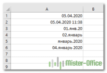 Как быстро вставить сегодняшнюю дату в Excel? — Это руководство показывает различные способы ввода дат в Excel. Узнайте, как вставить сегодняшнюю дату и время в виде статической метки времени или динамических значений, как автоматически заполнять столбец или строку…
  Количество рабочих дней между двумя датами в Excel — Довольно распространенная задача: определить количество рабочих дней в период между двумя датами – это частный случай расчета числа дней, который мы уже рассматривали ранее. Тем не менее, в Excel для…
If you use Excel regularly, I’m sure you’ve come across dates and times in your cells. Data often has a record of when it was created or updated, so knowing how to work with this data is essential.
Here are three key skills that you’ll learn in this tutorial:
- How to format dates in Excel so that they appear in your preferred style
- Formulas to calculate the number of days, months, and years between two dates
- An Excel date formula to log today’s date, and a keyboard shortcut to add the current time
Microsoft Excel can basically do anything with data, if you just know how. This tutorial is another key step to adding skills to your Excel toolbelt. Let’s get started.
Excel Date and Time Formulas (Quick Video Tutorial)
This screencast will walk you through how to work with dates and times in Excel. I cover formatting dates to different styles, as well as Excel date formulas to calculate and work with dates. Make sure to download the free Excel workbook with exercises that I’ve attached to this tutorial.
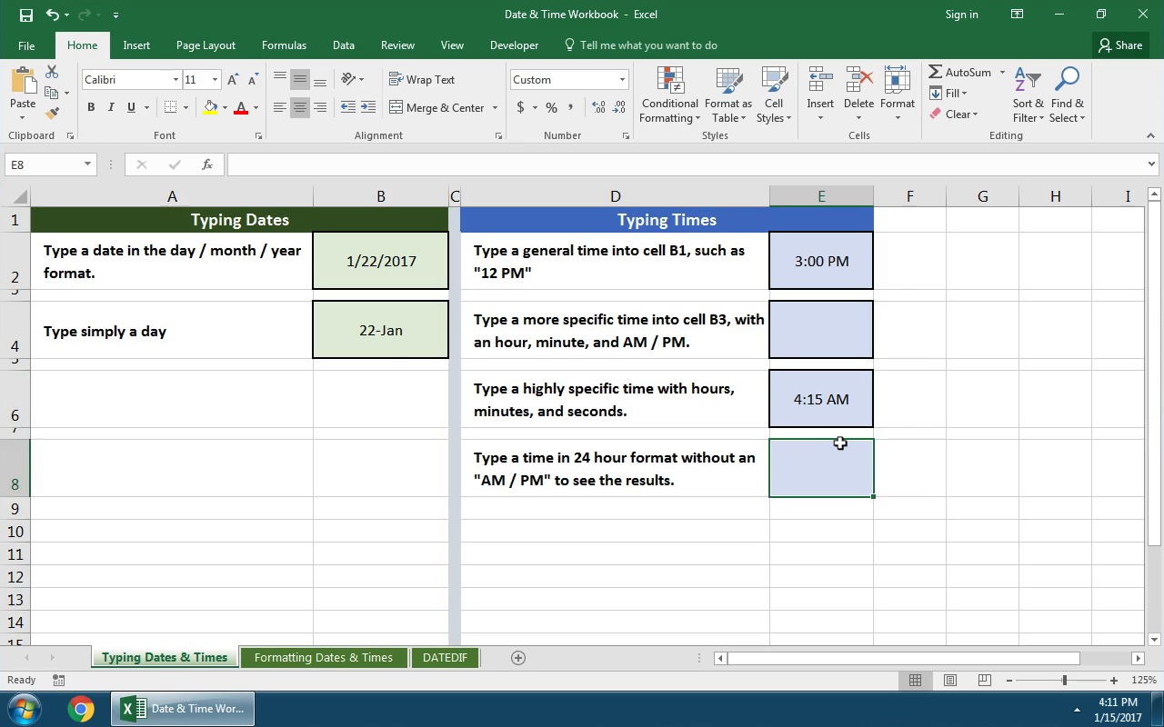
Keep reading for a written reference guide on how to format dates and times in Excel, and work with them in your formulas. I’ll even share several tips that weren’t covered in the screencast.
Typing Dates and Times in Excel
For this part of the tutorial, use the tab titled «Typing Dates & Times» in the example workbook.
One of the keys to working with dates and times in Excel is capturing the data correctly. Here’s how to type dates and times in your Excel spreadsheets:
1. How to Type Dates
I recommend typing dates in the same format that your system uses. For our American readers, a full date would be in the «day/month/year» format. European style dates are «month/day/year.»


When I’m typing dates, I always type in the full date with the month, day and year. If I only want to show the month and the year, I’ll simply format it that way (more on that in a minute.)
2. How to Type Times
It’s easy to type times in Excel. We can specify anything from just an hour of the day, to the exact second that something took place.
If I wanted to log the time as 4PM, I’d type «4 pm» into a cell in Excel and then press enter:


Notice once we press enter, Excel converts what we’ve typed into a hours : minutes: seconds data format.
Here’s how to log a more specific time in your spreadsheet:


The key is to use colons to separate the section of the time data, and then add a space plus «AM» or «PM.»
3. How to Type Date-Time Together
You can also type combinations of dates and times in Excel for highly specific timestamps.
To type a date-time combination, simply use what we’ve already learned about typing dates, and typing times.


Notice that Excel has converted the time to a 24 hour format when it’s used in conjunction with a date, by default. If you want to change the style of this date, keep reading.
Bonus: Excel Keyboard Shortcut for Current Time
One of my favorite Excel keyboard shortcuts inserts the current time into a spreadsheet. I use this formula often, when I’m noting the time I made a change to my data. Try it out:
Control + Shift + ;
Formatting Dates in Excel
For this part of the tutorial, use the tab titled «Formatting Dates & Times» in the example workbook.
What can you do when your dates are European style dates? That is, they’re in a day-month-year format, and you need to convert them to the more familiar month-day-year format?

In the screenshot above, what might surprise you is that all six of those cells contain exactly the same data — «1/22/2017.» What differs is how they’re formatted in Excel. The original data is identical, but it can be formatted to show in a variety of ways.
In most cases, it’s better to use formatting to modify the style of our dates. We don’t need to modify the data itself — just change how it’s presented.
Format Excel Cells
To change the appearance of our date and time data, make sure that you’re working on the Home tab of Excel. On the Ribbon (menu at the top of Excel), find the section labeled Number.
There’s a small arrow in the lower right corner of the section. Click it to open the Format Cells menu.


The Format Cells menu has a variety of options for styling your dates and times. You could turn «1/22/2017» into «Sunday, January 22nd» with just formatting. Then, you could grab the format painter and change all of your cell styles.


Spend some time exploring this menu and trying out the different styles for your Excel dates and times.
Get Data From Dates and Times
Let’s say that we have a list of data that has very specific dates and times, and we want to get simpler versions of those formulas. Maybe we have a list of exact transaction dates, but we want to work with them at a higher level, grouping them by year or month.
You can get the year from a date with this Excel formula:
=YEAR(CELL)


To get just the month from a date cell, use the following Excel formula:
=MON(CELL)


Find the Difference Between Dates and Times
For this part of the tutorial, use the tab titled «DATEDIF» in the example workbook.
While formats are used to change how dates and times are presented, formulas in Excel are used to modify, calculate, or work with dates and times programatically.
The DATEDIF formula is powerful for calculating differences between days. Give the formula two dates and and it will return the number of days, months, and years between two dates. Let’s look at how to use it.
1. Days Between Dates
This Excel date formula will calculate the number of days between two dates:
=DATEDIF(A1,B1,"d")
The formula takes two cells, separated by commas, and then uses a «d» to calculate the difference in days.


Here are some ideas for how you could use this Excel date formula to your advantage:
- Calculate the difference between today and your birthday to start a birthday countdown
- Use a DATEDIF to calculate the difference between two dates and divide your stock portfolio’s growth by the number of days to calculate the growth (or loss!) per day
2. Months Between Dates
DATEDIF also calculates the number of months between two dates. This date formula in Excel is very similar, but substitutes an «m» for «d» to calculate the difference in months:
=DATEDIF(A1,B1,"m")
However, there’s a quirk in the way Excel applies DATEDIF: it calculates whole months between dates. See the screenshot below.


To me, there are three months between January 1st and March 31st (all of January, all of February, and almost all of March.) However, because Excel uses whole months, it only considers January and February as completed, whole months, so the result is «2.»
Here’s my preferred way to calculate the number of months between two dates. We’ll find the date difference in days, and then divide it by the average number of days in a month — 30.42 .
=(DATEDIF(A1,B1,"d")/30.42)
Let’s apply our modified DATEDIF to two dates:


Much better. The output of 2.99 is very close to 3 full months, and this will be much more useful in future formulas.
The official Excel documentation has a complex method to calculate months between dates, but this is a simple and easy way to get it pretty close. Writing a good Excel formula is about finding the sweet spot of precision and simplicity, and this formula does both.
3. Years Between Dates
Finally, let’s calculate the number of years between two dates. The official way to calculate years between dates is with the following formula:
=DATEDIF(A1,B1,"y")
Notice that this is the same as our past DATEDIF formulas, but we’ve simply substituted the last part of the formula with «y» to calculate the number of years between two dates. Let’s see it in action:


Notice that this works like the DATEDIF for months: it counts only full years that have passed. I’d rather include partial years passing as well. Here’s a better DATEDIF for years:
=(DATEDIF(A1,B2,"d")/365)
Basically, we’re just getting the date difference in days, and then dividing it by 365 to calculate it as a year. Here’s the results:


DATEDIF is extremely powerful, but watch out for how it works: it’s going to only calculate full months or years that have passed by default. Use my modified versions for more precision in the results.
Bonus: Work Days Between Dates
The Excel date formulas covered above focus on the number of business days between dates. However, it’s sometimes helpful to just calculate the number of workdays (basically weekdays) between two dates.
In this case, we’ll use =NETWORKDAYS to calculate the number of workdays between two dates.
=NETWORKDAYS(A1,B1)
In the screenshot below, I show an example of using NETWORKDAYS. You can see the calendar showing how the formula calculated a result of «4.»


If you have known holidays in the timeframe that you want to exclude, check out the official NETWORKDAYS documentation.
Recap and Keep Learning
Dates and times are ubiquitous to spreadsheets. Excel date formulas and formatting options are helpful. The techniques in this tutorial can take your Excel skills to the next level so that you can incorporate date-driven data seamlessly into your spreadsheets.
You’ve added one skill to your Excel toolbox — why stop here? Chain Excel formulas and skills to create powerful spreadsheets. To keep learning more about working with Excel spreadsheets, check out these other resources:
- IF Statements are logic built into your spreadsheet that show results based on conditions. You could combine an IF Statement with a date range to show data based on a date or time. Check out this tutorial to learn them.
- You could combine the VLOOKUP tutorial with date and time formulas to match values based on a date or time.
- Find and Remove Duplicates is an Excel function used in combination with date and time data, as it’s often one of the best bits of data to check for duplicates.
How do you work with calendar and time data in your Excel spreadsheets? Are there are any Excel date or time formulas that I’m missing from this tutorial that you use regularly? If so, let me know in the comments.