
Excel for Microsoft 365 Excel for Microsoft 365 for Mac Excel 2021 Excel 2021 for Mac Excel 2019 Excel 2019 for Mac Excel 2016 Excel 2016 for Mac Excel 2013 Excel 2010 Excel 2007 More…Less
To make managing and analyzing a group of related data easier, you can turn a range of cells into an Excel table (previously known as an Excel list).

Note: Excel tables should not be confused with the data tables that are part of a suite of what-if analysis commands. For more information about data tables, see Calculate multiple results with a data table.
Learn about the elements of an Excel table
A table can include the following elements:
-
Header row By default, a table has a header row. Every table column has filtering enabled in the header row so that you can filter or sort your table data quickly. For more information, see Filter data or Sort data.

You can turn off the header row in a table. For more information, see Turn Excel table headers on or off.
-
Banded rows Alternate shading or banding in rows helps to better distinguish the data.
-
Calculated columns By entering a formula in one cell in a table column, you can create a calculated column in which that formula is instantly applied to all other cells in that table column. For more information, see Use calculated columns in an Excel table.
-
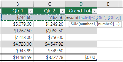
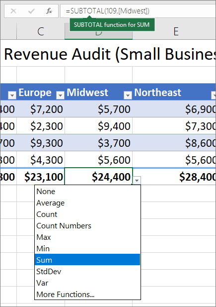
Total row Once you add a total row to a table, Excel gives you an AutoSum drop-down list to select from functions such as SUM, AVERAGE, and so on. When you select one of these options, the table will automatically convert them to a SUBTOTAL function, which will ignore rows that have been hidden with a filter by default. If you want to include hidden rows in your calculations, you can change the SUBTOTAL function arguments.
For more information, also see Total the data in an Excel table.
-
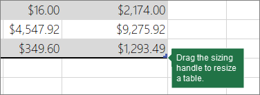
Sizing handle A sizing handle in the lower-right corner of the table allows you to drag the table to the size that you want.
For other ways to resize a table, see Resize a table by adding rows and columns.
Create a table
You can create as many tables as you want in a spreadsheet.
To quickly create a table in Excel, do the following:
-
Select the cell or the range in the data.
-
Select Home > Format as Table.
-
Pick a table style.
-
In the Format as Table dialog box, select the checkbox next to My table as headers if you want the first row of the range to be the header row, and then click OK.
Also watch a video on creating a table in Excel.
Working efficiently with your table data
Excel has some features that enable you to work efficiently with your table data:
-
Using structured references Instead of using cell references, such as A1 and R1C1, you can use structured references that reference table names in a formula. For more information, see Using structured references with Excel tables.
-
Ensuring data integrity You can use the built-in data validation feature in Excel. For example, you may choose to allow only numbers or dates in a column of a table. For more information on how to ensure data integrity, see Apply data validation to cells.
Export an Excel table to a SharePoint site
If you have authoring access to a SharePoint site, you can use it to export an Excel table to a SharePoint list. This way other people can view, edit, and update the table data in the SharePoint list. You can create a one-way connection to the SharePoint list so that you can refresh the table data on the worksheet to incorporate changes that are made to the data in the SharePoint list. For more information, see Export an Excel table to SharePoint.
Need more help?
You can always ask an expert in the Excel Tech Community or get support in the Answers community.
See Also
Format an Excel table
Excel table compatibility issues
Need more help?
Want more options?
Explore subscription benefits, browse training courses, learn how to secure your device, and more.
Communities help you ask and answer questions, give feedback, and hear from experts with rich knowledge.
Microsoft Excel is convenient for creating tables and doing calculations. Its working area is a set of cells to be filled with data. Consequently, the data can be formatted, used for building graphs, charts, summary reports.
For a beginner, working with tables in Excel may seem complicated at the first glance. It is differs considerably from the principles of table construction in Word. However, let us start from the very basics: creating and formatting tables. By the time you reach the end of this article, you will understand there is no better tool for creating tables than Excel.
Creating a table in Excel: a dummy’s guide
Working with Excel tables for dummies does not tolerate haste. There are different ways to create a table for a specific purpose, and each of them has its advantages. Therefore, let us start with assessing the situation visually.
Look carefully at the work sheet of the table processor:
It is a set of cells in columns and rows. Essentially, it’s a table. The columns are marked with letters. The rows are designated with numbers. There are no borders.
First of all, let’s learn to work with cells, rows and columns.
How to select a column and a row
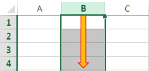
To select the entire column, left-click on the letter that marks it.
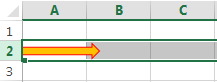
To select a row, click on the number it’s designated with.
To select several columns or rows, left-click on the name, hold down the button and drag the pointer.
To select a column with the help of hot keys, place the cursor in any cell of the column and press Ctrl + Space. The key combination Shift + Space is used to select a row.
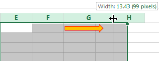
How to resize cells
If your information does not fit in the table, you need to resize the cells.
- You can move them manually by grabbing the cell boundary with the left mouse button.
- If the cell contains a long word, you can double-click on the boundary of the column/row. The program will expand its boundary automatically.
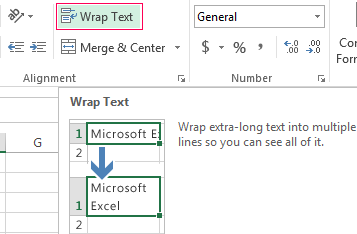
- If you need to increase the height of a row preserving the column width, use the button «Wrap Text» in the tool bar.
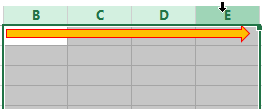
To change the column width and the row height in a certain range, resize 1 column/row (by dragging its boundaries manually) – and all the selected columns and rows will be resized automatically.
Important note. To go back to the previous size, you can press the «Undo Typing» button or the hot-key combination CTRL+Z. However, it works only if used immediately. Later on, it will not help.
To bring the rows to their initial boundaries, open the tool menu: «HOME»-«Format» and choose «AutoFit Row Height».
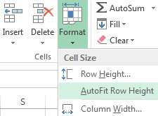
This method does not work for columns. Click «Format» — « AutoFit Row Width» Memorize this number. Select any cell in the column that needs to go back to the initial size. Click «Format» — «Column Width» again and enter the value suggested by the program (as a rule, it’s 8.43 – the number of characters in the Calibri font, size 11 pt). OK.
How to insert a column or row
Select the column/row to the right of/below the place where the insertion needs to be made. That is, the new column will appear to the left of the selected cell. The new row will be pasted above it.
Right-click on the cell and select «Insert» in the drop-down menu (or hit the hot-key combination CTRL+SHIFT+»=»).
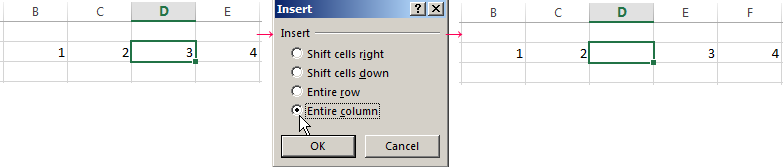
Select «Entire column» and press OK.
Hint. To insert a new column quickly, select a column in the desired position and hit CTRL+SHIFT+PLUS.
All these skills will come handy when building a table in Excel. You will need to resize the cells and insert rows/columns in the process.
Creating a table with formulas step by step
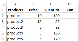
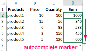
- Fill in the header manually by entering the column headings. Fill in the rows by entering your data. Apply the acquired knowledge in practice: expand the column boundaries, adjust the row height.
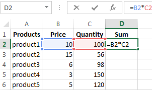
- To fill in the «Sum» column, place the cursor in its first cell. Enter «=». In such a way, we inform Excel: a formula will be here. Select the cell B2 (with the first price). Enter the multiplication symbol (*). Select the cell C2 (with the quantity). Press ENTER.
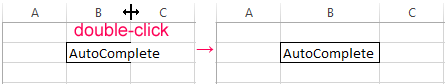
- When you hover the pointer over the cell containing the formula, a small cross will appear in its bottom right corner. It points out the autocomplete marker. Grab it with the left mouse button and drag it to the end of the column. The formula will be copied into every cell.
- Designate the boundaries of your table. Select the range containing your data. Click the button «HOME»-«Border» (on the main page in the «Font» menu). And click «All Borders».
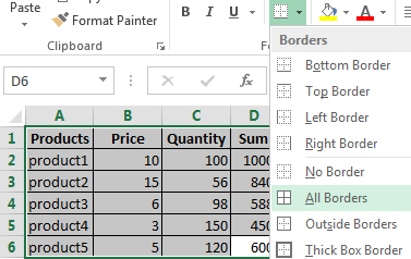
Now the column and row borders will be visible when you print the table.
The «Font» menu allows you to format the data in your Excel table the way you would do it in Word.
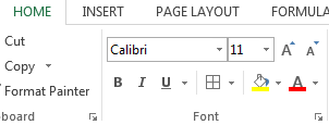
For example, change the font size and highlight the header in bold. You may also apply center alignment, word wrap, etc.
Creating a table in Excel: a step-by-step instruction
You already know the simplest way to create tables. However, Excel can offer a more convenient variant (in terms of the subsequent formatting and work with the data).
Let us construct a smart (dynamic) table:
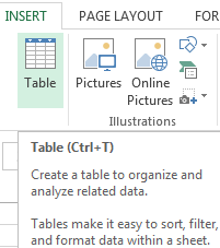
- Go to the «INSERT» tab – the «Table» tool (or press the hot-key combination CTRL+T).
- This will open a dialog window, in which you need to enter the data range. Check the box for a table with headings. Click OK. It’s no big deal if you don’t enter the proper range on the first try. The smart table is flexible, dynamic.
Important note. You can also take an alternative route: start with selecting the range of cells, then press the «Table» button.
Now enter your data into the ready framework. If you need an additional column, place the cursor in the heading cell. Make the entry and press ENTER. The range will expand automatically.

If you need additional rows, grab the autocomplete marker in the bottom right corner and drag it downward.
How to work with a table in Excel
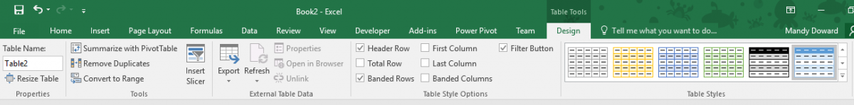
With the release of new versions of the program, working with tables in Excel has become more interesting and dynamic. After a smart table has been formed on the spreadsheet, the tool «TABLE TOOLS» — «DESIGN» becomes available.
Here you can name the table or resize it.
Various styles are available to you, as well as the opportunity to transform the table into a regular range or a consolidated sheet.
MS Excel dynamic electronic tables offer immense opportunities. Let us begin with the basic skills of data entry and autocompletion:
- Select a cell by clicking on it with the left mouse button. Enter the text/numeric value. Press ENTER. If you need to change the value, place the cursor in the cell again and enter the new data.
- When you enter a value repetitively, Excel will recognize it. You will only need to enter several symbols and press enter.
- In a smart table, to apply a formula to the entire column, enter it in the first cell. The program will copy the formula in other cells automatically.
- To calculate the totals, select the column containing the values plus an empty cell for the future total and click the «Sum» button (the «Editing» tool group on the «HOME» tab, or press the hot-key combination ALT+»=»).
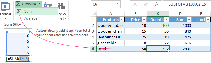
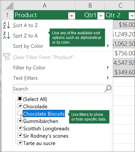
When you click on the little arrow to the right of every subheading in the header, you obtain access to the additional tools for working with the data in the table.
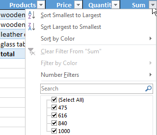
Sometimes the user has to work with huge tables, in which you need to scroll several thousand rows to see the totals. Deleting the rows is not an option (you will still need the data later). However, you can hide them. To this end, use number filters (depicted in the image above). Uncheck the values that need to be hidden.
What are Excel Tables?
Tables in Excel helps group related data into one or more rows and/or columns. Once a table is created, Excel assigns a unique name to the columns and the table itself. Such names are used as structured references, which make it easy to apply Excel formulas. Therefore, tables eliminate the need to create named ranges in Excel.
For example, the following image shows a usual data range on the left side and an Excel table on the right side. Notice the alternately colored excel rowsThe two different methods to add colour to alternative rows are adding alternative row colour using Excel table styles or highlighting alternative rows using the Excel conditional formatting option.read more and structured references (in cell J2) of the latter.
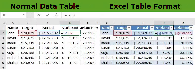
The purpose of creating tables is to make the data manageable, organized, and fit for analysis. Apart from structured references, tables offer several benefits like quick sorting and filtering, automatic expansion, easy formatting, readable formulas, and so on. Tables are extremely helpful when working with large databases.
Table of contents
- What are Excel Tables?
- How to Create Tables in Excel?
- How to Customize Tables in Excel?
- #1–Change the Name of the Table
- #2–Change the Color of the Table
- What are the Advantages of Creating Tables in Excel?
- #1–Creates Structured References Automatically
- #2–Is Dynamic in Nature
- #3–Makes it Easy to Work With PivotTables
- #4–Freezes Header Row Automatically
- #5–Helps add a Total Row Containing Functions
- #6–Eases Restoring to Usual Data Range Without Losing the Table Style
- #7–Helps add Slicers for Filtering Data
- #8–Assists in Creating Reports in Power BI
- How to Turn off Structured References in Excel?
- Frequently Asked Questions
- Recommended Articles
How to Create Tables in Excel?
You can download this Excel Tables Template here – Excel Tables Template
The steps to create a table in Excel are listed as follows:
- Ensure that the raw data does not contain any empty rows and/or columns. Further, each column should have a unique heading. If any two columns have the same headers, Excel automatically changes one of these headers once a table is created.
The raw data is shown in the following image.
Note: A column header should not contain any Excel formulas.

- Select any cell of the raw data and press the shortcut “Ctrl+T.” Both keys of the shortcut should be pressed together.
Note: Alternatively, after selecting a cell of the raw data, click “table” from the Insert tab of Excel. This option is in the “tables” group of the Excel ribbon.

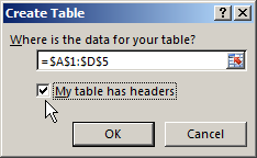
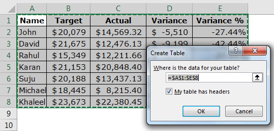
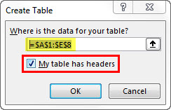
- The “create table” dialog box opens, as shown in the following image. Excel automatically selects the range for the table. Check whether this range is correct or not. If not, it can be edited.

- Select or deselect the checkbox of “my table has headers.” If selected, Excel will treat the content of the first row (row 1) as column headers.
In the preceding table, row 1 does contain column headers. So, we have selected the option “my table has headers.” Next, click “Ok.”

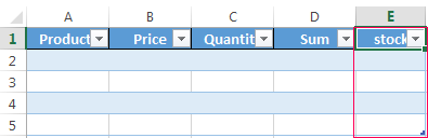
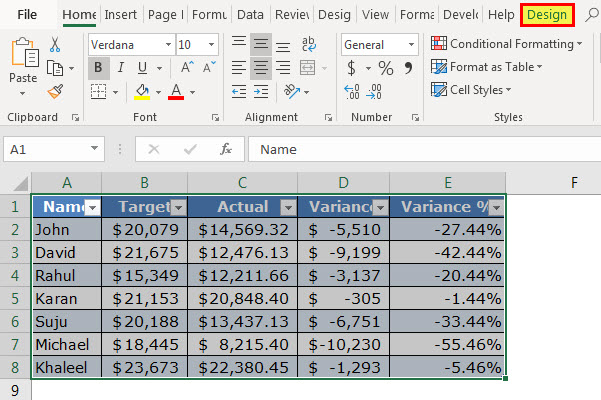
- An Excel table has been created. It is shown in the following image. Notice that the banded rows and filters (to the right of each column header) appear automatically.
Note: In Excel, banded rows are those in which color or shading is applied alternately.


How to Customize Tables in Excel?
A table can be customized by changing its name and/or the default color (or table style). Let us learn how this is done.
#1–Change the Name of the Table
When a table is created, Excel assigns a default name like “table1,” “table2,” etc., depending on whether it is the first or the second table of the current workbook.
Working with such default names may become confusing, especially when there are lots of tables. So, the solution is to assign unique names to each table.
The steps for changing the name of the Excel table are listed as follows:
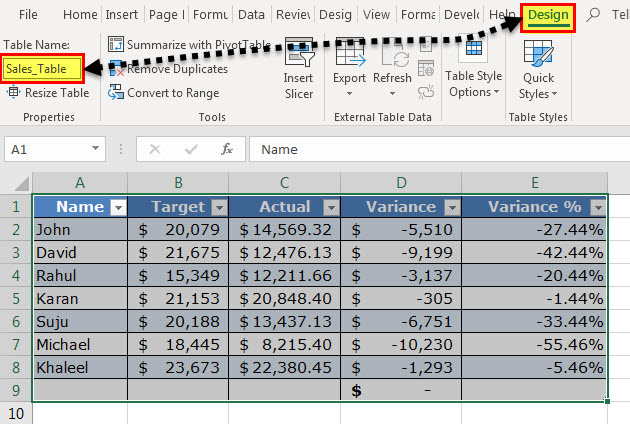
Step 1: Select the entire table. Once selected, the Design tab appears on the Excel ribbonRibbons in Excel 2016 are designed to help you easily locate the command you want to use. Ribbons are organized into logical groups called Tabs, each of which has its own set of functions.read more. This tab is shown within a red box in the following image.
Note: In place of the entire table, even if a single cell is selected, the Design tab will become visible.
Step 2: In the Design tab, perform the following tasks:
- Click inside the box under “table name.” This box is displayed in the “properties” group at the leftmost side of the ribbon.
- Enter the desired name in this box.
- Press the “Enter” key.
Our table has been named “Sales_Table.” This is shown in the following image.
Rules Governing the Table Names
While naming a table, the following points should be considered:
- The name should always begin with a letter, a backslash () or an underscore (_).
- The name cannot be the single letter “r” (or “R”) or “c” (or “C”).
- The name should not consist of any spaces. Instead, one can use an underscore (_) or a period (.) to separate the words.
- The name can contain numbers, but cell references should be avoided.
- The name can contain a maximum of 255 characters.
- The name of the table should be unique. In case of a duplicate name, a message will be displayed saying that a unique name should be chosen.
Note: A name is said to be duplicate if two tables within the same workbook have the same names. Further, Excel does not distinguish between the uppercase and lowercase letters in the name of a table. So, the names “abc” or “ABC” are considered the same by Excel.
#2–Change the Color of the Table
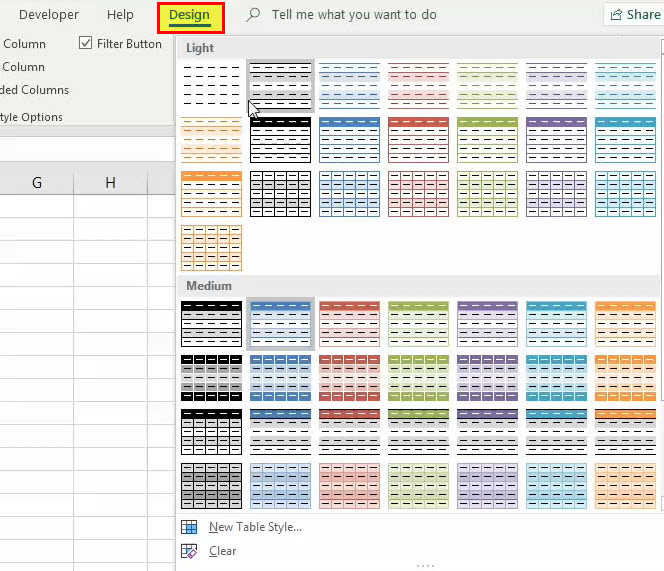
When a table is created, Excel assigns it a default color. To change the color of the table, its style needs to be changed. Excel displays a list of different table styles from which one can choose the desired option.
The steps to change the color (or style) of a table are listed as follows:
Step 1: Select either a cell of the table or the entire table. We have selected the latter. The Design tab becomes visible, as shown in the following image.

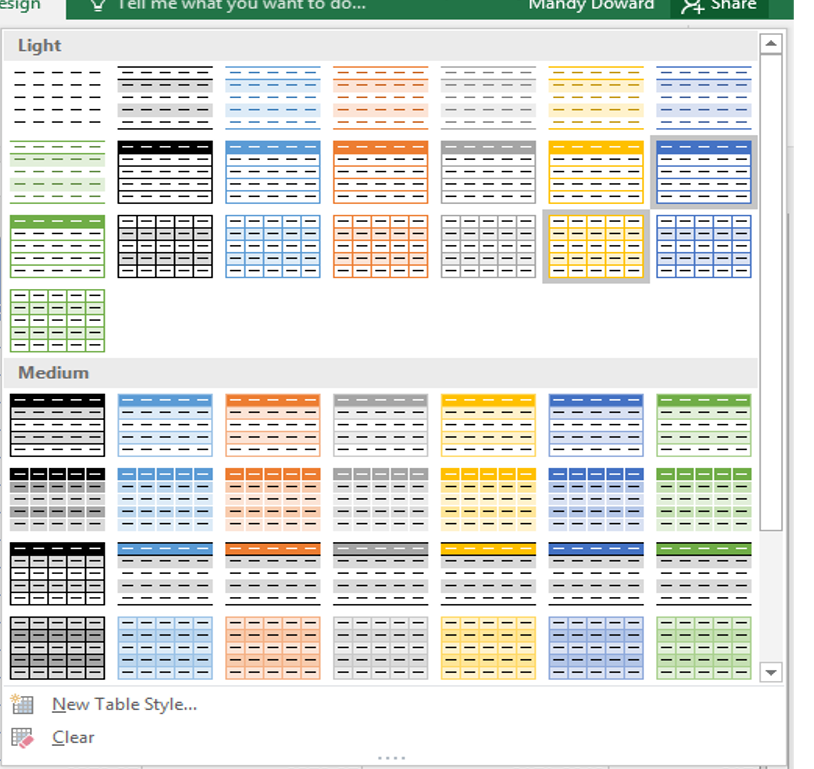
Step 2: Choose the desired color (or style) from the “table styles” group of the Design tab. To expand the list of table styles, click the “more” button displayed at the bottom right side. One can also click “new table style” to view more styles.
The following image shows the expanded list of table styles. Once the desired style is chosen, it will be applied to the entire table.
Note: The default table style of the workbook can be changed by the user. For making this change, perform the listed steps:
- Select the desired table style from the list of table styles.
- Right-click the selected table style and choose “set as default” from the context menu.
What are the Advantages of Creating Tables in Excel?
Let us discuss eight advantages of creating tables in Excel.
#1–Creates Structured References Automatically
An Excel table uses structured referencesIn Excel, structured references define data sets in columns by giving names instead of cell address. You may use the column name instead of the cell address in the formula; this makes work easier.read more for referencing one or more cells. This is in contrast with the direct cell addresses used in a normal data range. A structured reference is a combination of table and column names that are used in Excel formulasThe term «basic excel formula» refers to the general functions used in Microsoft Excel to do simple calculations such as addition, average, and comparison. SUM, COUNT, COUNTA, COUNTBLANK, AVERAGE, MIN Excel, MAX Excel, LEN Excel, TRIM Excel, IF Excel are the top ten excel formulas and functions.read more.
The major benefits of using structured references are listed as follows:
- They automatically update when new entries are added or deleted from the table.
- They are automatically created when one or more cells of the table are selected.
- They can be used both within and outside the table, thus making it easy to locate tables in a workbook.
- They are used to autofill the calculated columns. A calculated column is an additional column added to the existing Excel table. It uses a single formula that expands on its own in the remaining part of the column. This implies that when a formula is entered in one cell of a calculated column, it need not be dragged to the remaining cells of the column. Rather, the formula is automatically entered in all cells (called autofill), unlike a usual data range which requires one to drag the fill handleThe fill handle in Excel allows you to avoid copying and pasting each value into cells and instead use patterns to fill out the information. This tiny cross is a versatile tool in the Excel suite that can be used for data entry, data transformation, and many other applications.read more.
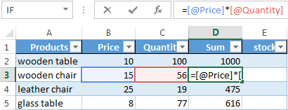
Example of point “d”: The range A2:B7 is an Excel table containing random numbers. To create column C as a calculated column, enter the SUM formula in cell C3, which adds the numbers of cells A3 and B3. Use structured references in this formula. Once the formula is entered, press the “Enter” key. The outcomes are stated as follows:
- The table (A2:B7) automatically expands to include column C.
- The range C4:C7 is automatically filled with the totals of each row of the table.
The preceding results will be obtained with both structured and regular references. This is because autofilling is a feature of Excel tables. However, with structured references, it is easy to read and understand the formula.
Note that if the user makes a change to the formula of the calculated column, the change is automatically replicated in the entire column.
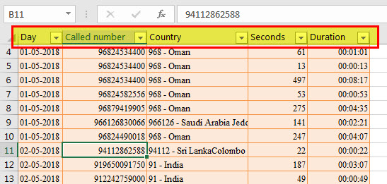
Example of structured references: In the following image, structured references have been used in the SUMIF formula. The “Calls_Table” is the name of the Excel table. “Day” and “duration” are the names of columns A and E respectively. The cell G2 is a direct cell referenceCell reference in excel is referring the other cells to a cell to use its values or properties. For instance, if we have data in cell A2 and want to use that in cell A1, use =A2 in cell A1, and this will copy the A2 value in A1.read more.
Note: In the following image, the black line pointing to cell G2 has been incorrectly placed. It should have pointed to “day,” which is the name of column A. So, please ignore the misplacement.

#2–Is Dynamic in Nature
Any new insertions to the cells below or to the right of the table are automatically included in the Excel table. This implies that the table expands to include such insertions. Likewise, the table contracts when one or more rows and/or columns are deleted from it. Due to automatic expansion and contraction, an Excel table is often considered a dynamic tableDynamic tables in Excel are ones in which the table automatically adjusts its size when a new value is inserted. It can be done in one of two ways: by using the offset function or by creating a data table from the table section.read more.
Expansion implies that the style, formatting, and formulas of the table are automatically applied to the new entries as well. This eliminates the need to format and edit the formulas of individual cells. By default, the formatting stays uniform throughout an Excel table.
Note that the formulas of the table are adjustable as they take into account structured references. In contrast, the formulas of a normal data range do not adjust with insertions or deletions of entries.
Note: To undo table expansion, press the keys “Ctrl+Z” together.
#3–Makes it Easy to Work With PivotTables
It is advised to create a PivotTableA Pivot Table is an Excel tool that allows you to extract data in a preferred format (dashboard/reports) from large data sets contained within a worksheet. It can summarize, sort, group, and reorganize data, as well as execute other complex calculations on it.read more from an Excel table. The major reasons the source data should be an Excel table are listed as follows:
- A PivotTable automatically updates with any changes in the source table. Since Excel tables are dynamic, the data range of the PivotTable also becomes dynamic.
- A single cell of the source table can be selected prior to inserting a PivotTable. In contrast, when the source data is a usual data range, the entire range (or dataset) needs to be selected prior to inserting a PivotTable.
For instance, in the following image, a single cell of the source table has been selected before clicking the “PivotTable” option from the Excel Insert tabIn excel “INSERT” tab plays an important role in analyzing the data. Like all the other tabs in the ribbon INSERT tab offers its own features and tools. Under Insert Tab we have several other groups including tables, illustration, add-ins, charts, Power map, sparklines, filters, etc.read more. Notice that in “table/range,” the name of the source table is reflected.

When one scrolls downwards in a worksheet, the table headers are visible at all times. This is because these headers are automatically fixed or frozen at their respective places.
Fixed headers prevent the user from going back to the top row (row 1) again and again. Such frozen headers can be seen within a red rectangle in the following image.
Notice that the user has scrolled downwards such that rows 4 to 13 are visible along with the header row.
Note: To see the frozen header row, ensure that a cell of the table is selected before scrolling.
#5–Helps add a Total Row Containing Functions
An Excel table shows various functions in the total row. For displaying this row, perform the following steps:
- Select any cell of the Excel table. The Design tab appears on the Excel ribbon.
- From the Design tab, select the checkbox of “total row” displayed in the “table style options” group.
The total row is added immediately below the Excel table. Select any cell of this row to see a drop-down arrow on the right side. When this arrow is clicked, a list containing functions appears, as shown in the following image.
Once a function is selected from the list, the respective formula is automatically entered and the output is shown in a cell of the total row.
Notice that row 9 of the following image is the total row. Further, if a function is selected in cell D9, the corresponding output will also be displayed in this cell. The formula will be visible in the formula bar of the worksheet.

#6–Eases Restoring to Usual Data Range Without Losing the Table Style
An Excel table can be quickly converted to a usual data range. This serves as a benefit when the user requires only the table style and not the functionality of the table. For such conversion, follow either of the listed steps:
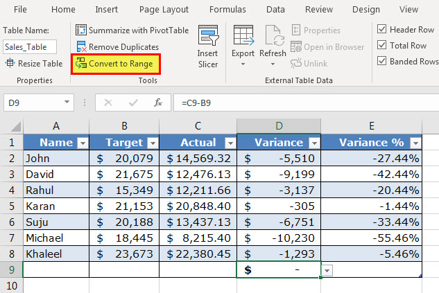
- Select any cell of the table. From the Design tab, click “convert to range” in the tools group.
- Select any cell of the table and right-click it. From the context menu, choose “table” followed by “convert to range.”
The “convert to range” feature of the first pointer is shown in the following image. Once an Excel table is converted to a usual data range, the existing structured references are replaced with the regular cell references. However, the data and formatting of the table are retained in the usual data range.
Note: The “convert to range” feature can be used only when the data to be converted is in the form of an Excel table.
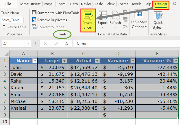
#7–Helps add Slicers for Filtering Data
A slicer helps filter the data of an Excel table. It displays buttons that can be selected or deselected to indicate whether an item is included or excluded from the filter.
Slicers are available in Excel 2013 and the newer Excel versions. The steps to add a slicer to a table are listed as follows:
- Select either a cell within the table or the entire table.
- From the Design tab, select “insert slicer” from the “tools” group.
- The “insert slicer” dialog box opens. Next, select the checkboxes of the columns for which the slicer needs to be created.
- Click “Ok.”
One can have a slicer for each column of the Excel table. Once slicers appear in the worksheet, they can be moved, resized, and formatted according to the requirement.
With a slicer, one can filter and view only particular items (or entries) of the table. To view multiple items of a column, press and hold the “Ctrl” key while selecting the items in the respective slicer.
The following image shows the “insert slicer” option of the Design tab.
Note 1: A slicer can also be added from the “filters” group of the Insert tab of Excel. Click “slicer” in this group and thereafter follow the steps “c” and “d” listed above.
Note 2: A slicer can be used only if the data is in the form of an Excel table.
#8–Assists in Creating Reports in Power BI
Excel tables serve as a source from which data is entered in the Power BI tool. Power BI is a business intelligence tool that helps convert unrelated sources of data into meaningful reports and dashboards. The process of creating reports works as follows:
- Create and upload Excel tables to Power BI.
- Create a report in Power BI by adding visualizations.
- Share the report with other Power BI users or office colleagues.
Excel tables are a preferred data source in Power BI due to the following reasons:
- They allow quick access to the tabular format of the dataset.
- They help ease comparisons within a dataset.
- They can be easily edited and organized prior to being uploaded in Power BI.
How to Turn off Structured References in Excel?
The steps to turn off structured references in Excel are listed as follows:
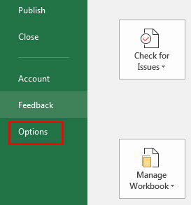
Step 1: Click the File tab of Excel. It is displayed within a red box in the following image.

Step 2: Select “options” shown in the following image.
Step 3: The “Excel options” dialog box opens. Click “formulas” appearing on the left side of the window. Deselect the checkbox of “use table names in formulas.” This is shown in the following image.
Next, click “Ok.” The structured references will be turned off in Excel.
Note: By changing this setting, the structured references used in the existing formulas of the Excel table are not removed. However, the new formulas applied to the table will contain regular cell references instead of structured references. If regular cell references are required in existing formulas too, they will have to be edited manually.
Further, whether the structured references are turned on or off, the changed setting will be applied to all workbooks that the user is working on.

Frequently Asked Questions
1. What are Excel tables and how are they created?
An Excel table displays the data in a tabulated format. Every column should have unique headers (or names) according to the kind of data they contain. Such headers are placed in the top row of the table. The table may or may not be named by the user.
If the columns and table are not named by the user, Excel assigns default names to both of them. These names are used as structured references in all formulas applied within or outside the table (that contain a table reference).
To create a table in Excel, select any cell of the dataset and press the keys “Ctrl+T” or “Ctrl+L.”
2. How to join two tables in Excel?
Two tables that have a common column can be joined with the help of the VLOOKUP function of Excel. The formula is stated as follows:
“=VLOOKUP(lookup_value,entire_lookup_table,return_column,FALSE)”
For instance, the first table is named “table1” and the second table is named “table2.” To pull the data of a single column of “table2” in “table1,” enter the following formula:
“=VLOOKUP($A2,table2,3,FALSE)”
This formula looks up the value of cell A2 in “table2.” It returns an exact match from the third column of “table2.”
One can use either regular or structured references in the given formula. By selecting the cell of the “lookup_value” and the range of the “entire_lookup_table,” Excel will automatically enter structured references in the VLOOKUP formula.
Note 1: Enter the given formula in the first cell to the immediate right of the first table. Once entered, press the “Enter” key. The Excel table expands to include the new column. Consequently, the outputs of the entire column are displayed in the first table.
Note 2: For the given formula to work, the column containing the “lookup_value” should be common to both tables. Moreover, the lookup column (containing the “lookup_value”) should be the leftmost column of the second table. The return column (containing the value to be returned) of the second table should be to the right of the lookup column.
3. When should Excel tables be used and how to locate them in a workbook?
Excel tables should be used in the following situations:
• To arrange data in a tabular format
• To facilitate comparisons of data values
• To improve the readability of the dataset
• To ease data analysis and eventually assist in decision-making
To locate tables in a workbook, click the downward arrow appearing on the right side of the name box. It shows the names of all the tables of the workbook. Clicking on any of these names will select that particular table.
Recommended Articles
This has been a guide to tables in Excel. Here, we explain how to create/insert/customize Excel tables along with examples and advantages. You may also look at these useful functions of Excel–
- Delete Pivot Table ExcelTo delete a pivot table in Excel, you must first select it. Then go to the Analyze menu tab under the Design and Analyze menu tabs and select actions. Then, from the Select option’s drop-down option, select Entire Pivot Table to delete it.read more
- Refresh Pivot Table in ExcelTo refresh pivot tables, you may use the following methods — refresh pivot table by changing data source, refresh pivot table using right click option, auto-refresh pivot table using VBA Code, refresh pivot table when you open the workbook.read more
- Data Table in Excel
- Excel Merge Tables We can use a number of different methods to merge tables in Excel, including the VLOOKUP function, the INDEX function, and the MATCH function.read more
You may think that an Excel Workbook already provides a table of data to you, and in a sense it does, an area consisting of Rows and Columns, with column and row headings and values.
It is, however, possible to create formal Tables from ranges of cells on an Excel worksheet.
Why would we want to do this?
Well, here are a few reasons:
- Automatic Filtering & Sorts
- Predefined formatting and colour schemes to choose from
- Colour banded rows
- Table Headings
- Single table name available to address all the data in that region of a worksheet (dynamic table size)
- Automatic Totals
- Slicers
There are many other benefits too.
Let’s take a look.
Create A Table From a Range of Cells
The screen shot below shows some raw sales data that has been pasted into an Excel Worklbook.
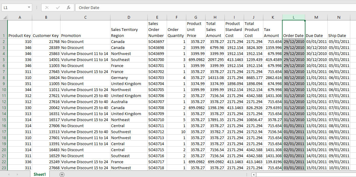
We can quite happily work on this data without converting it to a table. We can:
- Add columns
- Add rows
- Enter formulae into Cells
- Format cells
- Add Validation Rules to cells.
And so on ……
But, ……..
Tables give us just a little bit more.
We will create a table from the above data.
On the Insert ribbon there is a Table option – shown in the screen shot below:
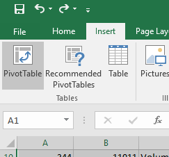
Highlight the area of the worksheet that contains the data along with the column headings and then click on Table:
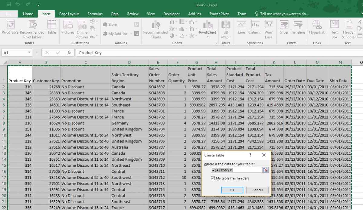
A dialog pops up where you can confirm or alter the area containing the table data. You can also indicate if the table includes column headings (it does in this example).
Clicking on OK results in the table being created with a default Table Style:
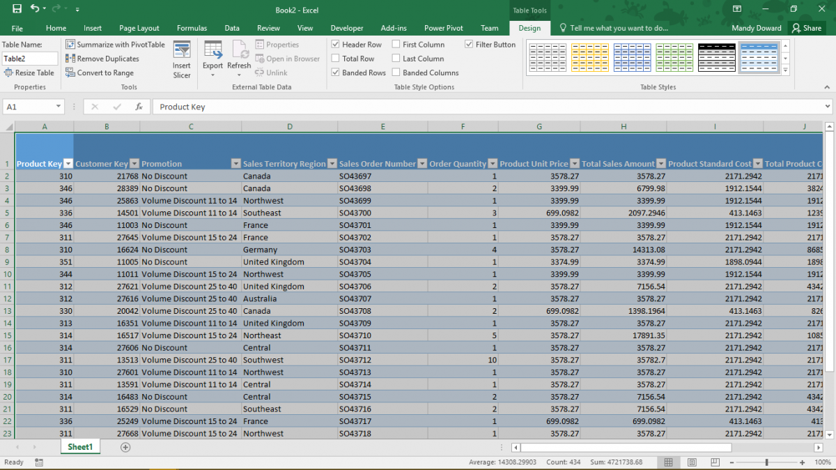
Immediate benefits are:
- Formatted with a Table Style
- Banded formatting for alternate row shading
- Headings that remain frozen at the top of the table as you scroll down records
- Automatic filter drop downs for each column in the table
- Sorting options via the drop downs for each column in the table
- Table Name that can be used to address the whole table
Table Styles & Column Banding
The default blue based table style can be changed via the Table Tools Design Ribbon.
The Table Styles part of the ribbon offers quite a few options for formatting the table:
We will select one of the green themes:
The default styles include Column Banding to make it easier to identify values from a row.
Column Banding can be turned off via the Table Tools Design ribbon:
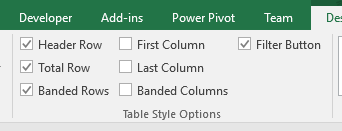
You can see that the Table Style Options section of the ribbon offers tick boxes for Banded Rows (on by default) and Banded Columns.
In the following example we have deselected Banded Rows and selected Banded Columns.
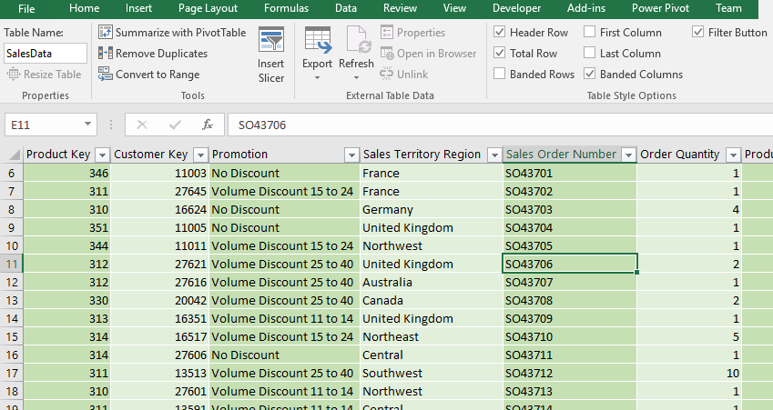
Table Headings
In the screen shot below you can see the default table headings:
When you scroll down the data rows the headings stay displayed at the top of the worksheet area (where you would normally see the Row Letters):
Table Filters & Sort Operations
Every column in the table gets automatic filtering and sort options via the drop down seen to the right of each column name:
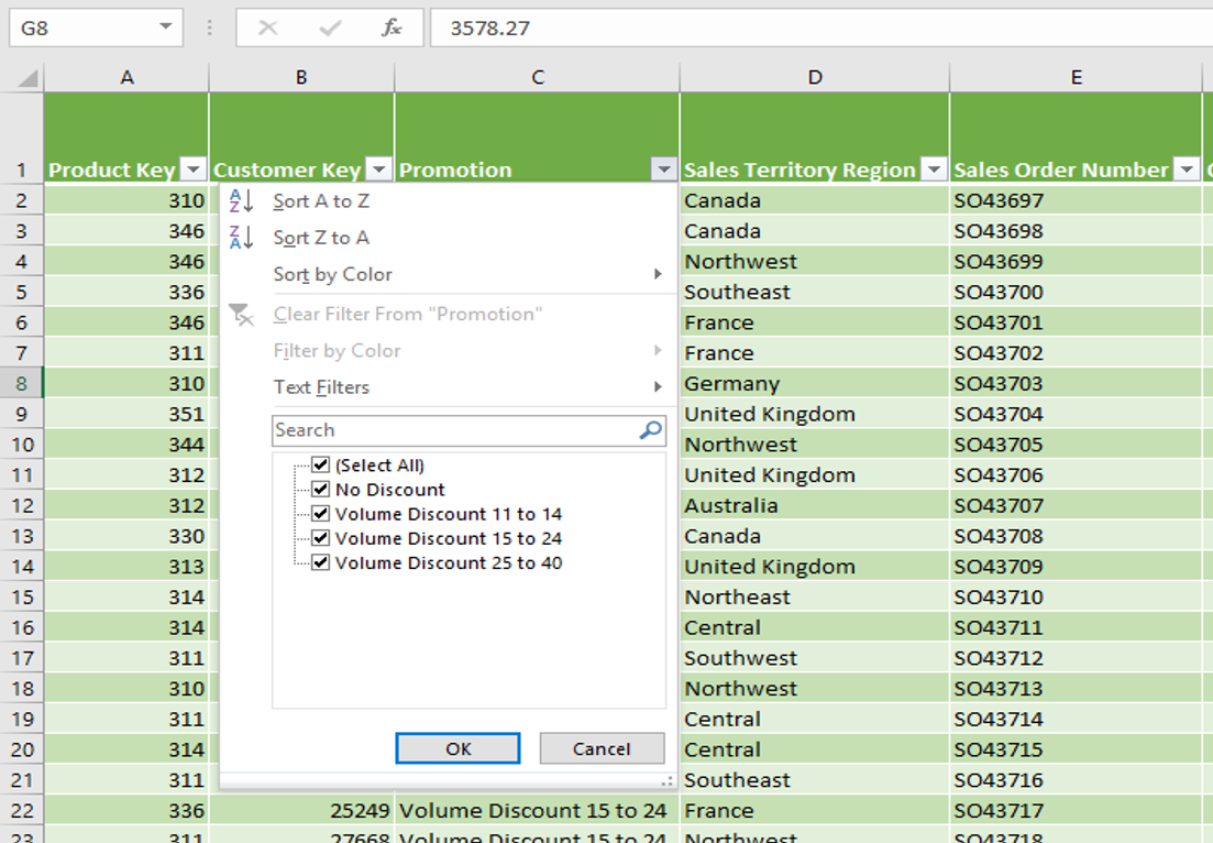
Table Name
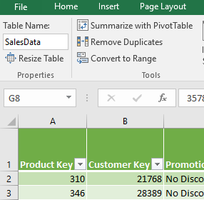
The Table is automatically given a name. This can be changed as shown in the following screen shot, to make it a more easily remembered and relevant name. The following example shows a table renamed as SalesData.
This table name can then be used in any formula or tool that requires the range of cells in the table. This range will also be dynamic so that as the table grows with new rows and columns they will be included in the referencing formulae and tools.
For example, we can use the table name when using the table data as the source for a Pivot Table:
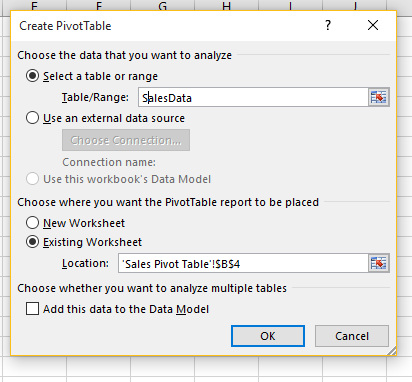
Note that we have used the table name, SalesData, in the Table/Range field instead of referencing the Worksheet and Cell Range.
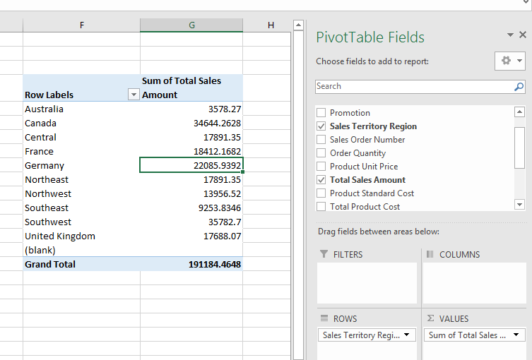
Here is a sample Pivot Table from this source:
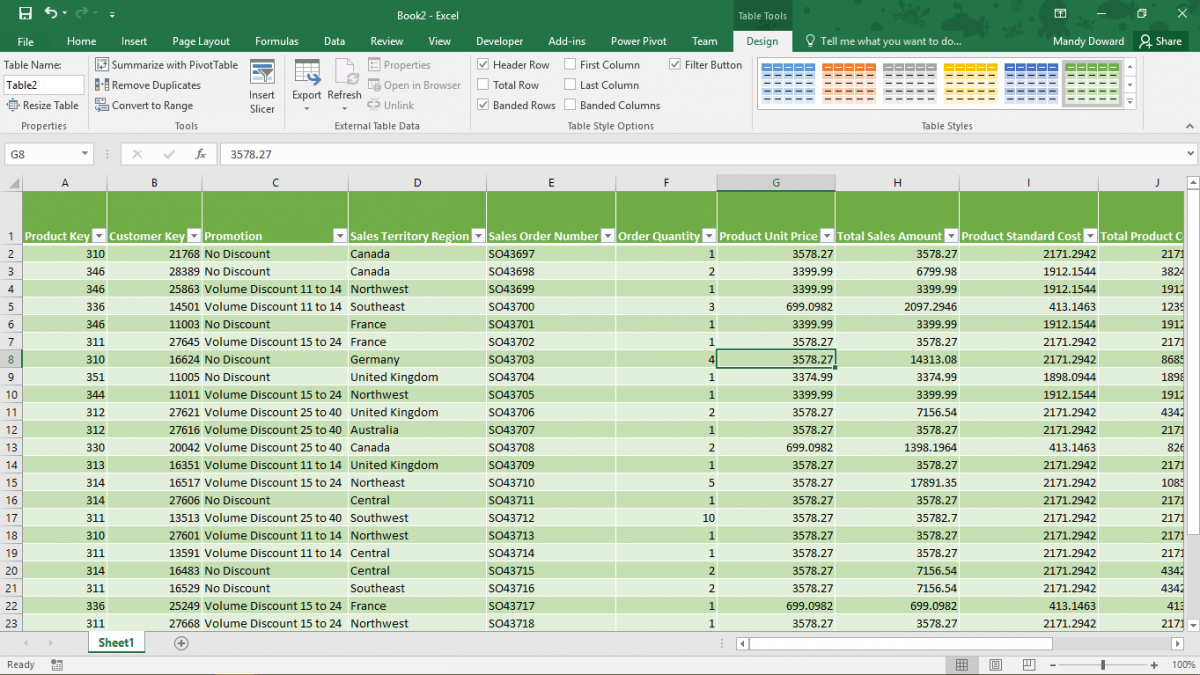
Adding Automatic Totals to an Excel Table
On the Table Tools Design Menu the Table Style Options group has a “Total Row” tick box.
If you tick this box a total row is added to the bottom of the table.
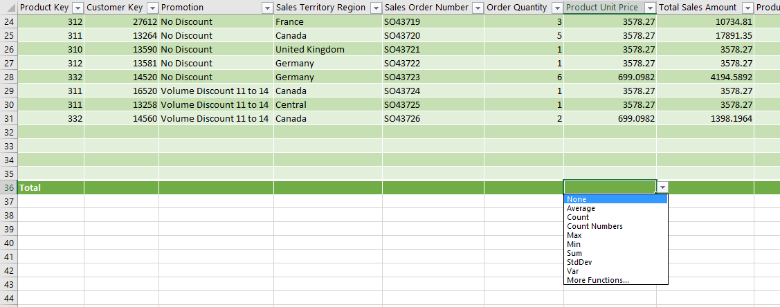
Once the total row has been added you can click in any of the cells in this row and an arrow will appear to the right of it enabling you to access a list of available aggregate functions to choose from. This is shown in the above sreen shot.
The following example shows an average has been added to the Product Unit Price and a total has been added to the Total Sales Amount column:
As new rows are added to the table the totals are automatically updated.
Another big benefit of Excel Table Total Rows is that if filtering is in place the aggrgate function results are automatically updated to reflect the filtered rows rather than just displaying the overall aggregate values.
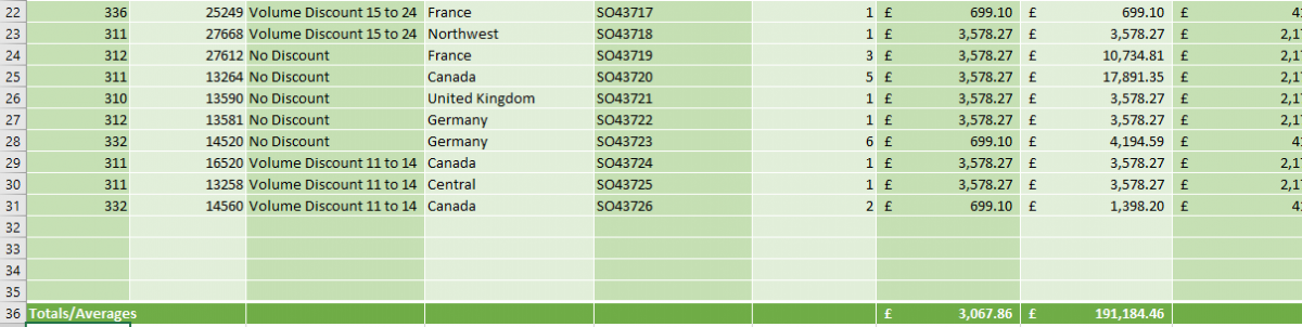
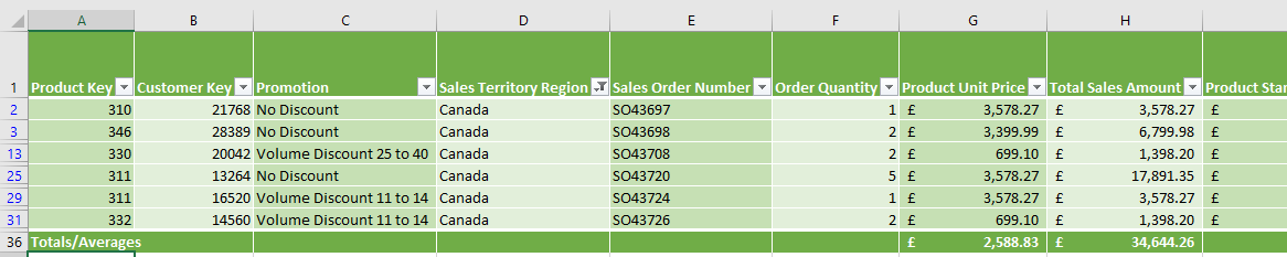
In the following example there is a filter on the Sales Territory Region column, so the Totals row is showing the average product price for Canada and the total sales amount for Canada:
..
Using Slicers With Excel Tables to Filter Data
Slicers are a wonderful way of filtering records. Typically they are used wioth Pivot Tables and Pivot Charts to slice and dice to looik at different sections of business data, whether that be a specific product, a specific set of years or regions, etc.
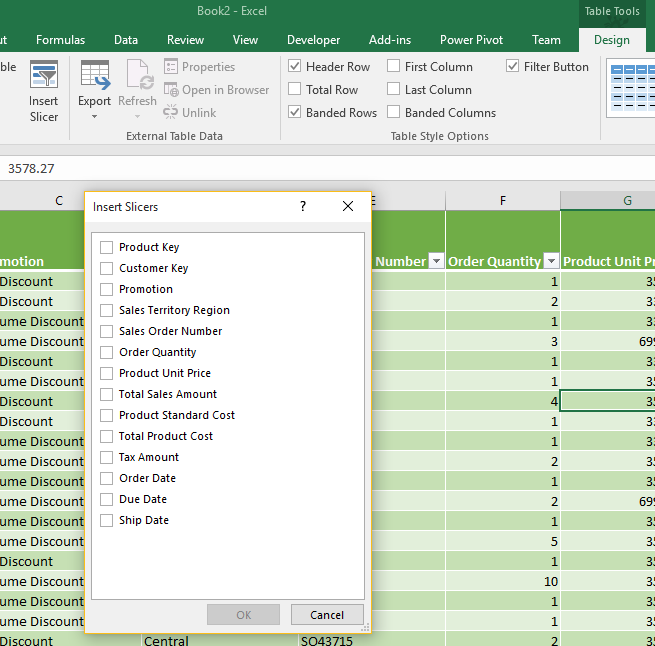
Slicers can be used with Excel Tables too. With the cursor located in a cell that belongs to your Excel table select the Table Tools Design ribbon. In the Tools section of the ribbon you will see an “Insert Slicer” option.
A dialog will open enabling you to select any of the available table columns to be added as slicers:
In the following example you can see that we selected the Promotion column and a slicer has been added to the worksheet:
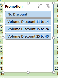
The four promotion values that appear in the table data are listed and selected by default. Filtering of the table can be implemented by clicking on promotion values in the slicer – the records in the table the slicer is linked to will automatically be updated to refelct the filter. More than one value can be selected using a <CTRL> click.
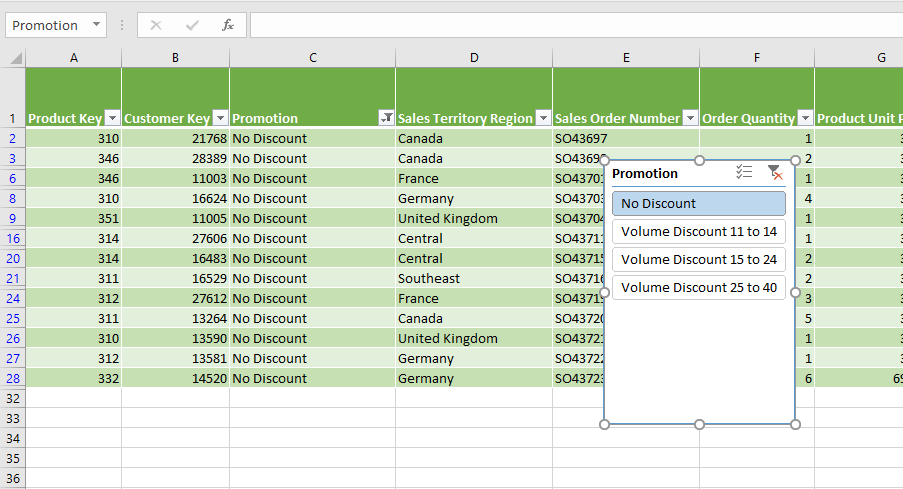
We can see that the slicer has “No Discount” selected and the table indicates a filter on the Promotion column (note the funnel icon to the right of the column name).
You can have many slicers associated with a table.
I hope you have found this article useful.
If you would like to learn more about working in Excel click here to view our courses and dates avaliable.
Did you know that all of our courses are available to attend virtually through platforms such as Teams and Zoom. To find out more about any of our courses or virtual training please email our Sales Director Keith on keith.doward@ptr.co.uk and he would be happy to assist you.
In this post, we’re going to learn everything there is to know about Excel Tables!
Yes, I mean everything and there’s a lot.
This post will tell you about all the awesome features Excel Tables have and why you should start using them.
What is an Excel Table?
Excel Tables are containers for your data.
Imagine a house without any closets or cupboards to store your things, it would be chaos! Excel tables are like closets and cupboards for your data, they help to contain and organize data in your spreadsheets.
In your house, you might put all your plates into one kitchen cupboard. Similarly, you might put all your customer data into one Excel table.
Tables tell excel that all the data is related. Without a table, the only thing relating the data is proximity to each other.
Ok, so what’s so great about Excel Tables other than being a container to organize data? A lot actually. This post will tell you about all the awesome features tables have and should convince you to start using them.
Video Tutorial
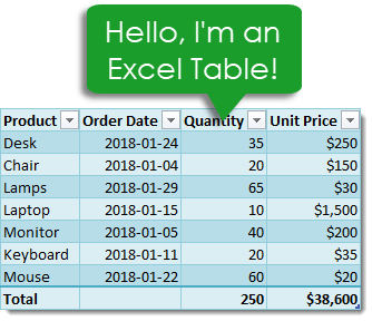
The Parts of a Table
Throughout this post, I’ll be referring to various parts of a table, so it’s probably a good idea that we’re both talking about the same thing.
This is the Column Header Row. It is the first row in a table and contains the column headings that identify each column of data. Column headings must be unique in the table, they cannot be blank and they cannot contain formulas.
This is the Body of the table. The body is where all the data and formulas live.
This is a Row in the table. The body of a table can contain one or more rows and if you try to delete all the rows in a table a single blank row will remain.
This is a Column in the table. A table must contain at least one column.
This is the Total Row of the table. By default, tables don’t include a total row but this feature can be enabled if desired. If it’s enabled, it will be the last row of the table. This row can contain text, formula or remain blank. Each cell in the total row will have a drop down menu that allows selection of various summary formula.
Create a Table from the Ribbon
Creating an Excel Table is really easy. Select any cell inside your data and Excel will guess the range of your data when creating the table. You’ll be able to confirm this range later on. Instead of letting Excel guess the range you can also select the entire range of data in this step.
With the active cell inside your data range, go to the Insert tab in the ribbon and press the Table button found in the Tables section.
The Create Table dialog box will pop up. Excel guesses the range and you can adjust this range if needed using the range selector icon on the right hand side of the Where is the data for your table? input field. You can also adjust this range by manually typing over the range in the input field.
Checking the My table has headers box will tell Excel the first row of data contains the column headers in your table. If this is unchecked Excel will create generic column headers for the table labelled Column 1, Column 2 etc…
Press the Ok button when you’re satisfied with the data range and table headers check box.
Congratulations! You now have an Excel table and your data should look something like the above depending on the default style of your tables.
Contextual Table Tools Design Tab
Whenever you select a cell inside a table, you will notice a new tab appear in the ribbon labelled Table Tools Design. This is a contextual tab and only appears when a table is selected. When the active cell moves outside the table, the tab will disappear again.
This is where all the commands and options related to tables will live. This is where you’ll be able to name your table, find table related tools, enable or disable table elements and change your table’s style.
Create a Table with a Keyboard Shortcut
You can also create a table using a keyboard shortcut. The process is the same as described above but instead of using the Table button in the ribbon you can press Ctrl + T on your keyboard. It’s easy to remember since T is for Table!
There is actually another keyboard shortcut that you can use to create tables, Ctrl + L will also do the same thing. This is a legacy from when tables were called lists (L is for List).
Name a Table
Anytime you create a new table Excel will give it an initial generic name starting with Table1 and increasing sequentially. You should always rename your table with a descriptive and short name.
Not all names are allowed. There are a few rules for a table name.
- Each table must have a unique name within a workbook.
- You can only use letters, numbers and the underscore character in a table name. No spaces or other special characters are allowed.
- A table name must begin with either a letter or an underscore, it can not begin with a number.
- A table name can have a maximum of 255 characters.
Select any cell inside your table and the contextual Table Tools Design tab will appear in the ribbon. Inside this tab you can find the Table Name under the Properties section. Type over the generic name with your new name and press the Enter button when finished to confirm the new name.
Rename a Table
Renaming a table you’ve already named is the same process as naming a table for the first time. If you think about it, when you first name a table you’re actually renaming it from the generic name of Table1 to a new name.
So go back to the Table Tools Design tab and type your new name over the old one in the Table Name and press Enter. Easy, and the name is changed.
Changing your table name this way requires navigating to your table and selecting a cell within it, so it can be tedious if you need to rename a lot of tables across different sheets in your workbook. Instead, you can change any of your table names without going to each table using the Name Manager.
Go to the Formula tab and press the Name Manager button in the Defined Names section. You’ll be able to see all your named objects here. The table objects will have a small table icon to the left of the name. You can filter to show only the table objects using the Filter button in the upper right hand corner and selecting Table Names from the options.
You can then edit any name by selecting the item and pressing the Edit button. You’ll be able to change the name and add some comments to describe the data in your table.
Navigate Tables with the Name Box
You can easily navigate to any table in your workbook using the name box the the left of the formula bar. Click on the small arrow on the right side of the name box and you will see all table names in the workbook listed. Click on any of the tables listed and you will be taken to that table.
Convert a Table Back to a Normal Range
Ok, you changed your mind and don’t want your data inside a table anymore. How do you convert it back into a regular range?
If changing it to a table was the last thing you did, Ctrl + Z to undo your last action is probably the quickest way.
If it wasn’t the last thing you did, then you’re going to need to use the Convert to Range command found in the Table Tools Design tab under the Tools section.
You’ll be prompted to confirm that you really want to convert the table to a normal range. Noooooo, don’t do it, tables are awesome!
If you click on yes, then all the awesome benefits from tables will be gone except for the formatting design. You’ll need to manually clear this from the range if you want to get rid it. You can do this by going to the Home tab then pressing the Clear button found in the Editing section, then selecting Clear Formats.
This can also be done from the right click menu. Right click anywhere in the table and select Table from the menu and then Convert to Range.
Select the Entire Column
If your data is not inside a table then selecting an entire column of the data can be difficult. The usual way would be to select the first cell in the column and then hold Ctrl + Shift then press the Down arrow key. If the column has blank cells, then you might need to press the Down arrow key a few times until you reach the end of the data.
The other option is to select the first cell and then use the scroll bar to scroll to the end of your data then hold the Shift key while you select the last column.
Both options can be tedious if you have a lot of data or there are a lot of blanks cells in the data.
With a table, you can easily select the entire column regardless of blank cells. Hover the mouse cursor over the column heading until it turns into a small arrow pointing down then left click and the entire column will be selected. Left click a second time to include the column heading and any total row in the selection.
Another way to quickly select the entire column is to place the active cell cursor on any cell in the column and press Ctrl + Space. This will select the entire column excluding the column header and total row. Press Ctrl + Space again to include the column headers and total row.
Select the Entire Row
Selecting the entire row is just as easy. Hover the mouse cursor over the left side of the row until it turns into a small arrow pointing left then left click and the entire row will be selected. This works on both the column heading row and total row.
Another way to quickly select the entire row is to place the active cell cursor on any cell in the row and press Shift + Space.
Select the Entire Table
It’s also possible to select the entire table and there are a couple different ways to do this.
You can place the active cell cursor inside the table and press Ctrl + A. This will select the entire body of the table excluding the column headers and total row. Press Ctrl + A again to include the column headers and total row.
Hover the mouse over the top left hand corner of the table until the cursor turns into a small black diagonal right and downward pointing arrow. Left click once to select only the body. Left click a second time to include the header row and total row.
You can also select the table with the mouse. Place the active cell inside the table and then hover the mouse cursor over any edge of the table until it turns into a four way directional arrow then left click. This will also select the column headers and total row.
Select Parts of the Table from the Right Click Menu
You can also select rows, columns or the entire table using the right click menu. Right click anywhere on the row or column you want to select then choose Select and pick from the three options available.
Add a Total Row
You can add a total row which allows you to display summary calculations in the last row of your table.
Adding summary calculations at the bottom of your data can be dangerous as they might end up getting included by accident in a pivot table using the data. This is another advantage of tables, as the total row won’t be included in any pivot tables created with the table.
To enable the total row, go to the Table Tools Design tab and check the Total Row box found in the Table Style Options section.
You can temporarily disable the total row without losing the formulas you added to it. Excel will remember the formulas you had and they will appear when you enable it again.
Each cell in the total row has a drop down menu that allows you to pick various aggregating functions to summarize the column of data above.
You can also enter your own formulas. I’ve entered a SUMPRODUCT formula in the Unit Price total to sum the Quantity x Unit Price to calculate a total sale amount. Formulas don’t have to return a number, they can also be text results.
Constant numerical or text values are also allowed anywhere in the total row. In fact the leftmost column will usually contain the text Total by default.
Add a Total Row with a Right Click
You can also add the total row with a right click. Right click anywhere on the table and the choose Table and Total Row from the menu.
Add a Total Row with a Keyboard Shortcut
Another way to quickly add the total row is to place the active cell cursor inside your table and use the Ctrl + Shift + T keyboard shortcut.
Disable the Column Header Row
The column header row is enabled by default, but you can disable it. This doesn’t delete the column headers, it’s essentially like hiding them as you will still reference columns based on the column header name.
Go to the Table Tools Design tab and uncheck the Total Row box found in the Table Style Options section.
Add Bold Format to the First or Last Columns
You can enable a bold formatting on either your first or last column to highlight it and draw attention to them over other columns.
Go to the Table Tools Design tab and check either of the First Column or Last Column boxes (or both) found in the Table Style Options section.
Add Banded Rows or Columns
Banded rows are already enabled by default, but you can turn them off if you want. Banded columns are disabled by default, so you need to enable them if you want them.
To enable or disable either, go to the Table Tools Design tab and check or uncheck the Banded Rows or Banded Columns boxes found in the Table Style Options section.
I generally find banded rows are the most useful and if you enable banded columns at the same time, the table starts to look a little messy. I recommend one or the other and not both at the same time.
- Table with no banded rows or columns.
- Table with banded rows only.
- Table with banded columns only.
- Table with both banded rows and columns.
Table Filters
By default, the table filters option is enabled. You can disable them from the Table Tools Design tab by unchecking the Filter Button box found in the Table Style Options section.
You can also toggle the filters on or off from the active table by using the regular filter keyboard shortcut of Ctrl + Shift + L.
If you left click on any of the filters, it will bring up the familiar filter menu where you can sort your table and apply various filters depending on the type of data in the column.
The great thing about table filters is you can have them on multiple tables in the same sheet simultaneously. You will need to be careful though as filtered items in one table will affect the other tables if they share common rows. You can only have one set of filters at a time in a sheet of data without tables.
Total Row with Filters Applied
When you select a summary function from the drop down menu in the total row, Excel will create the corresponding SUBTOTAL formula. This SUBTOTAL formula ignores hidden and filtered items. So when you filter your table these summaries will update accordingly to exclude the filtered values.
Note that the SUMPRODUCT formula in the Unit Price column still includes all the filtered values while the SUBTOTAL sum formula in the Quantity column does not.
Column Headers Remain Visible When Scrolling
If you scroll down while the active cell is in a table, its column headers will remain visible along with the filter buttons. The table’s column headings will get promoted into the sheet’s column headings where we would normally see the alphabetic column name.
This is extremely handy when dealing with long tables as you won’t need to scroll back up to the top to see the column name or use the filters.
Automatically Include New Rows and Columns
If you type or copy and paste new data into the cells directly below a table, they will automatically be absorbed into the table.
The same thing happens when you type or copy and paste into the cells directly to the right of a table.
Automatically Fill Formulas Down the Entire Column
When you enter a formula inside a table it will automatically fill the formula down the entire column.
Even when a formula has already been entered and you add new data to the row directly below the table any existing formulas will automatically fill.
Editing an existing formula in any of the cells will also update the formula in the entire column. You’ll never forget to copy and paste down a formula again!
Turn Off the Auto Include and Auto Fill Settings
You can turn off the feature that automatically adds new rows or columns and fills down formulas.
Go to the File tab and select Options. Choose Proofing then press the AutoCorrect Options button. Navigate to the AutoFormat As You Type tab in the AutoCorrect dialog box.
Unchecking the Include new rows and columns in table option allows you to type directly underneath or to the right of a table without it absorbing the cells.
Unchecking the Fill formulas in tables to create calculated columns option means the formulas in a table will no longer automatically fill down the column.
Resize with the Handle
Every table comes with a Size Handle found in the bottom rightmost cell of the table.
When you hover the mouse over the handle, the cursor will turn into a double-sided diagonally slanting arrow and you can then click and drag to resize the table. You can either expand or contract the size. Data will be absorbed into the table or removed from it accordingly.
Resize with the Ribbon
You can also resize the table from the ribbon. Go to the Table Tools Design tab and press the Resize Table command in the Properties section.
The Resize Table dialog box will pop up and you’ll be able to select a new range for your table. Use the range selector icon to select a new range. You can select either a larger or smaller range, but The table headers will need to remain in the same row and the new table range must overlap the old table range.
Add a New Row with the Tab Key
You can add a new blank row to a table with the Tab key. Place the active cell cursor inside the table on the cell containing the sizing handle and press the Tab key.
The tab key act like a carriage return and the active cell is taken to the rightmost cell on a new line that’s added directly below.
This is a handy shortcut to know because when the total row is enabled, it’s not possible to add a new row by typing or copying and pasting data directly below the table.
Insert Rows or Columns
You can insert extra rows or columns into a table with a right click. Select a range in the table and right click then choose Insert from the menu. You can then either choose to insert Table Columns to the Left or Table Rows Above.
Table Columns to the Left will insert the number of columns selected to the left of the selection and the number of rows in the selection is ignored.
Table Rows Above will insert the number of rows selected just above the selection and the number of columns in the selection is ignored.
Delete Rows or Columns
Deleting rows or columns has a similar story to inserting them. Select a range in the table and right click then choose Delete from the menu. You can then either choose to delete Table Columns or Table Rows.
Formats in a Table Automatically Apply to New Rows
When you add new data to your table, you don’t need to worry about applying formatting to match the rest of the data above. Formatting will automatically fill down from above if the formatting has been applied to the entire column.
I’m not just talking about the table style formats. Other formatting like dates, numbers, fonts, alignments, borders, conditional formatting, cell colours etc. will all automatically fill down if they’ve been applied to the whole column.
If you’ve formatted all your numbers as a currency in a column and you add new data, it too will get the currency format applied to it.
You never need to worry about inconsistent formatting in your data.
Add a Slicer
You can add a slicer (or several) to a table for an easy to use filter and visual way to see what items the table is filtered on.
Go to the Table Tools Design tab and press the Insert Slicer button found in the Tools section.
Change the Style
Changing the styling of a table is quick and easy. Go to the Table Tools Design select a new style from the selection found in the Table Styles section. If you left click the small downward arrow on the right hand side of the styles palette, it will expand to show all available options.
These table styles apply to the whole table and will also apply to any new rows or columns added later on.
There are many options to choose from including light, medium and dark themes. As you hover over the various selections, you’ll be able to see a live preview in the worksheet. The style won’t actually change until you click on one though.
You can even create your own New Table Style.
Set a Default Table Style
You can set any of the styles available as the default so that when you create a new table you don’t need to change the style. Right click on the style you want to set as the default and then choose Set As Default from the menu.
Unfortunately, this is a workbook level setting and will only affect the current workbook. You will need to set the default for each workbook you create if you don’t want the application default option.
Only Print the Selected Table
When you place the active cell cursor inside a table and then try to print, there is an option to only print the selected table. Go to the Print menu screen by either going to the File tab and selecting Print or using the Ctrl + P keyboard shortcut, then select Print Selected Table in the settings.
This will remove any items from the print area that are not in the table.
Structured Referencing
Tables come with a useful feature called structured referencing which helps to make range references more readable. Ranges within a table can be referred to using a combination of the table name and column headings.
Instead of seeing a formula like this =SUM(D3:D9) you might see something like this =SUM(Sales[Quantity]) which is much easier to understand the meaning of.
This is why naming your table with a short descriptive name and column headings is important as it will improve the readability of the structured references!
When you reference specific parts of a table, Excel will create the reference for you so you don’t need to memorize the reference structure but it will help to understand it a bit.
Structured references can contain up to three parts.
- This is the table name. When referencing a range from inside the table this part of the reference is not required.
- These are range identifiers and identify certain parts of the reference for a table like the headers or total row.
- These are the column names and will either be a single column or a range of columns separated by a full colon.
Example of structured References for a Row
=Sales[@[Unit Price]]will reference a single cell in the body.=Sales[@[Product]:[Unit Price]]will reference part of the row from the Product column to the Unit Price column including all columns in between.=Sales[@]will reference the full row.
Example of Structured References for Columns
=Sales[Unit Price]will reference a single column and only include the body.=Sales[[#Headers],[#Data],[Unit Price]]will reference a single column and include the column header and body.=Sales[[#Data],[#Totals],[Unit Price]]will reference a single column and include the body and total row.=Sales[[#All],[Unit Price]]will reference a single column and include the column header, body and total row.
Example of Structured References for the Total Row
=Sales[#Totals]will reference the entire total row.=Sales[[#Totals],[Unit Price]]will reference a cell in the total row.=Sales[[#Totals],[Product]:[Unit Price]]will reference part of the total row from the Product column to the Unit Price column including all columns in between.
Example of Structured References for the Column Header Row
=Sales[#Headers]will reference the entire column header row.=Sales[[#Headers],[Order Date]]will reference a cell in the column header row.=Sales[[#Headers],[Product]:[Unit Price]]will reference part of the column header row from the Product column to the Unit Price column including all columns in between.
Example of Structured References for the Table Body
=Saleswill reference the entire body.=Sales[[#Headers],[#Data]]will reference the entire column header row and body.=Sales[[#Data],[#Totals]]will reference the entire body and total row.=Sales[#All]will reference the entire column header row, body and total row.
Using Intellisense
One of the great things about a table is the structured references will appear in Intellisense menus when writing formulas. This means you can easily write a formula using the structured references without remembering all the fields in your table.
After typing the first letter of the table name, the IntelliSense menu will show the table name among all the other objects starting with that letter. You can use the arrow keys to navigate to it and then press the Tab key to autocomplete the table name in your formula.
If you want to reference a part of the table, you can then type a [ to bring up all the available items in the table. Again, you can navigate with the arrow keys and then use the Tab key to autocomplete the field name. Then you can close the item with a ].
Turn Off Structured Referencing
If you’re not a fan of being forced to use the structured referencing system, then you can turn it off. Any formulas that have been entered using the structured referencing will remain and they will still work the same. You’ll also still be able to use structured references, Excel just won’t automatically create them for you.
To turn it off, go to the File tab and then select Options. Choose Formulas on the side pane and then uncheck the Use table names in formulas box and press the Ok button.
Summarize with a PivotTable
You can create a pivot table from your table in Table Tools Design tab, press the Summarize with PivotTable button found in the Tools section. This will bring up the Create PivotTable window and you can create a pivot table as usual.
This is the same as creating a pivot table from the Insert tab and doesn’t give any extra options specific to tables.
Remove Duplicates from a Table
You can create remove duplicate rows of data from your table in Table Tools Design tab, press the Remove Duplicates button found in the Tools section. This will bring up the Remove Duplicates window and delete duplicate values for one or more columns in the table.
This is the same as removing duplicates from the Data tab and doesn’t give any extra options specific to tables.
About the Author
John is a Microsoft MVP and qualified actuary with over 15 years of experience. He has worked in a variety of industries, including insurance, ad tech, and most recently Power Platform consulting. He is a keen problem solver and has a passion for using technology to make businesses more efficient.
Excel Tables are one of the most interesting and useful features in Excel. If you need a range that expands to include new data, and if you want to refer to data by name instead of by address, Excel Tables are for you. This article provides an introduction and overview.
1. Creating a table is fast
You can create an Excel Table in less than 10 seconds. First, remove blank rows and make sure all columns have a unique name, then put the cursor anywhere in the data and use the keyboard shortcut Control + T. When you click OK, Excel will create the table.

2. Navigate directly to tables
Like named ranges, tables will appear in the namebox dropdown menu. Just click the menu, and select the table. Excel will navigate to the table, even if it’s on a different tab in a workbook.

3. Tables provide special shortcuts
When you convert regular data to an Excel Table, almost every shortcut you know works better. For example, you can select rows with shift + space, and columns with control + space. These shortcuts make selections that run precisely to the edge of the table, even when you can’t see the edge of the table. Watch the video below for a quick rundown.
Video: Shortcuts for Excel tables
4. Painless drag and drop
Tables make it much easier to rearrange data with drag and drop. After you’ve selected a table row or column, simply drag to a new location. Excel will quietly insert the selection at the new location, without complaining about overwriting data.


Note: you must select the entire row or column. For columns, that includes the header.
5. Table headers stay visible
One frustration when working with a large set of data is that table headers disappear as you scroll down the table. Tables solve this problem in a clever way. When column headers scroll off the top of the table, Excel silently replaces worksheet columns with table headers.

6. Tables expand automatically
When new rows or columns are added to an Excel Table, the table expands to enclose them. In a similar way, a table automatically contracts when rows or columns are deleted. When combined with structured references (see below) this gives you a dynamic range to use with formulas.

7. Totals without formulas
All tables can display an optional Total Row. The Total Row can be easily configured to perform operations like SUM and COUNT without entering a formula. When the table is filtered, these totals will automatically calculate on visible rows only. You can toggle the Total Row on and off with the shortcut control + shift + T.

8. Rename a table anytime
All tables are automatically assigned a generic name like Table1, Table2, etc. However, you can rename a table at any time. Select any cell in the table and enter a new name on the Table Tools menu.

9. Fill formulas automatically
Tables have a feature called calculated columns that makes entering and maintaining formulas easier and more accurate. When you enter a standard formula in a column, the formula is automatically copied throughout the column, with no need for copy and paste.


10. Change formulas automatically
The same feature also handles formula changes. If you make a change to the formula anywhere in a calculated column, the formula is updated throughout the entire column. In the screen below, the tax rate has been changed to 7% in one step.

11. Human-readable formulas
Tables use a special formula syntax to refer to parts of a table by name. This feature is called «structured references». For example, to SUM a column called «Amount» in a table called «Orders», you can use a formula like this:
=SUM(Orders[Amount])

12. Easy dynamic ranges
The single biggest benefit of tables is that they automatically expand as new data is added, creating a dynamic range. You can easily use this dynamic range in your formulas. For example, the table in the screen below is named «Properties». The following formulas will always return correct values, even as data is added to the table:
=ROWS(Properties)
=MAX(Properties[Price])
=MIN(Properties[Price])

13. Enter structured references with the mouse
An easy way to enter structured references in formulas is to use the mouse to select part of the table. Excel will automatically enter the structured reference for you. In the screen below, the price column was selected after entering =MAX(

14. Enter structured references by typing
Another way to enter structured references is by typing. When you type the first few letters of a table in a formula, Excel will list matching table names below.

Use the arrow keys to select and the TAB key to confirm. To enter a column name, enter an opening square bracket ([) after the table name follow the same process — type a few letters, select with arrow keys, and use TAB to confirm.

Video: Introduction to Structured References and Tables
15. Check structured references with a formula
You can quickly check a structured reference with the formula bar. For example, the following formula will select data in the «Address» column in the «Properties» table shown above:
=Properties[Address]
And this formula will select the headers of the table:
=Properties[#Headers]
Video: How to query a table with formulas
Video: How to use SUMIFS with a table
16. Change table formatting with one click
All Excel tables have a style applied by default, but you can change this at any time. Select any cell in the table and use the Table Styles menu on the Table Tools tab of the ribbon. With one click, the table will inherit the new style.

17. Remove all formatting
Table formatting is not a requirement of Excel tables. To use a table without formatting, select the first style in the styles menu, which is called «None».

Tip: you can use this style to remove all table formatting before converting a table back to a normal range.
18. Override local formatting
When you apply a table style, local formatting is preserved by default. However, you can optionally override local formatting if you want. Right-click any style and choose «Apply and Clear formatting»:

19. Set a default table style
You can right-click any style and choose «Set as Default». New tables in the same workbook will now use the default you set.

Note: to set a default table style in new workbooks, create a custom start-up template as described in this article. In the template file, set the default table style of your choice.
20. Use a Table with a pivot table
When you use a table as the source for a pivot table, the pivot table will automatically stay up to date with changes in data. Watch the video below to see how this works.
Video: Use a table for your next pivot table
21. Use a table to create a dynamic chart
Tables are a great way to create dynamic charts. New data in the table will automatically appear in the chart, and charts will exclude filtered rows by default.
Video: How to build a simple dynamic chart
22. Add a slicer to a table
Although all tables get filter controls by default, you can also add a slicer to a table, to make it easy to filter data with large buttons. To add a slicer to a table, click the Insert Slicer button on the Design tab of the Table Tools menu.

The table below has a slicer for Department:

23. Get rid of a table
To get rid of a table, use the Convert to Range command on the Table Tools tab of the ribbon.

You might be surprised to see that converting a table back to a normal range doesn’t remove formatting. To remove table formatting, first apply the «None» table style, then use «Convert to Range».
How to Use Tables in Excel Step-By-Step With Examples (2023)
Not that you cannot get along in Excel without using tables – but if you yet don’t know what Excel tables are, you’re missing out on something very big 💥
Excel table is an amazing tool that will automate most of the operations that you’d want to perform on your dataset.
It is a named cell range that is a little too advanced when it comes to updating formulas, running totals, copying formulas, filtering, and sorting data.
The guide below will teach you all about Excel tables. So continue reading 🚀
And as you scroll down, do not forget to download our sample workbook here to tag along with the guide.
What is an Excel table?
An Excel table is a named range that has a variety of features to manage and analyze data.
You can use it to run a calculated column, total rows, filtering, sorting, expansion, and whatnot. To help your curiosity, let us quickly show what an Excel table looks like 👀

Generally, a table is only a two-dimensional representation of data in the form of rows and columns 📝
Excel tables were introduced in Excel 2007 and are available in all next versions of Excel up to Excel 365.
How to create a table in Excel
Creating a table in Excel is the easiest of all. Let’s make one and see how this works.
We have some data in the image below. Though it still looks like a table, note that this is not an Excel table yet.

To convert it into an Excel table 👇
- Click anywhere on the table.
- Go to the Insert Tab > Table.

If you’re more of a keyboard person, simply press down the Control Key + T to launch the create table dialog box ⌨
- The Create Table dialog box will automatically identify the cell range to be converted into a table.

However, if that’s not your table exactly, you can manually adjust the range 🚴♀️
- Check the box for “My data has headers”. This refers to table headers.

- And Click Okay.
Your data is now converted into an Excel table and the default table style is applied 😍

Filtering Excel table data
Now that we’ve created a table out of our dataset, let’s see what we can do with it.
Our table has a list of sale transactions. Let’s filter out the sale transactions for Product A only 🅰
To do that:
- Click on the drop-down icon in the Products header.

- This will launch the Filter menu, as shown below.

- Unselect all the products and only select Product A.

- And swish! We now only have the sales for Product A 🧙♀️

Similarly, you can filter the sales for any particular date or color by using the filtering option for tables.
Pro Tip!
The filter feature of Excel can be used without tables even. But for that, you need to manually select each column and apply filters to it 🥴
Excel tables bring you the advantage of an integrated Data Filter. However, if you don’t want your table to have them, that’s alright.
You can remove filters from your table in Excel by selecting the table > Table Design > Uncheck the Filter Button.
Sorting Excel table data
Excel tables also allow users to sort the data in their Excel tables in ascending or descending order 🔀
For example, let’s try sorting the sales in our table in descending order (largest to the smallest value). To do that:
- Click on the drop-down icon in the Amount header 📌

- From the drop-down menu, select the option “Sort Largest to Smallest”.

And look at the magic! The table looks all new instantly. The sale transactions are now organized in descending order in terms of the sale amount 🏆

You can do the same for dates – let’s sort them in ascending order.
- From the drop-down menu above, select “Oldest to Newest”.

And see how the entire table is reorganized along with the dates 📅

All the sale transactions are now arranged date-wise (from the oldest date to the newest one).
Format an Excel table
When you first create a table in Excel, it will appear in the default table format of Excel. Which you may or may not like 🙈
If it’s the latter case, don’t worry. You can reformat your table in a hundred ways. To change the format of your Excel table:
- Click anywhere on the table.
A new tab will appear on your Ribbon by the name of Table Design 🎨
- Go to the Table Design tab > Table Styles.

Those are not all.
- Click on the small arrow to the right of the table styles box to launch this menu further.

Too many. Aren’t they?
- Hover your cursor on these designs to get a quick preview of how your table will look under each design.
- Once you have chosen the design for your table, click on it to have it applied to your table.
Just like we have applied the light blue table style here 🥶

Summary row
Yeah, a summary row or you may call it the total row that you can add to your Excel table very easily 🔔
Let’s take the example of our table above, where we have the amount for sales in the last column. If you need to perform any operation on these sales – you don’t need to write functions from a scratch.
The Excel table will do that for you. See here.
- Select the table.
- Go to Table Design Tools > Check the option for Total Row.

- Check out your table for an additional row. Do you see the totals there in the right bottom?

Not just the totals – but you can perform any function here 🤯
- Select the summary row for any column, and a drop-down arrow will appear.

- Click on it to launch the menu of functions.

6. Choose any of these operations by clicking on it to have it applied to the subject column
For example, let’s try calculating the average sales by clicking on the Average option from the drop-down list.
And here comes the average for the above numbers 🔥

Pro Tip!
If you go to the formula bar to see the function running on the backend of the summary row, you’d find the SUBTOTAL function instead of the simple AVERAGE function 🤔

Why is it used, and why haven’t we used the simple SUM / AVERAGE functions?
Learn that by reading our blog on the SUBTOTAL function. Link in the Other Resources Section. 👇
That’s it – Now what?
Until now, we have learned almost everything about Excel tables. From converting a simple data range into a table to filtering, sorting, and formatting it.
Hope you enjoyed it just as much as we did. If you did, don’t just stop here 📍
Excel tables make a great tool that will ease your data storing and sorting jobs by 100 times. But that’s just one tool in Excel, and there’s a whole library of functions, features, and tools in Excel for you to explore.
To learn everything about Excel, master Excel functions first. Particularly, the key Excel functions like the VLOOKUP, SUMIF, and IF functions.
My 30-minute free email course will take you through the (and many more) functions of Excel. Click here to enroll now.
Frequently asked questions
To name a table in Excel:
- Go to the Formulas Tab > Name Manager > Table1 (or by the name with which your table is saved).
- Under the Name dialog box, add a suitable name for your table (without space characters).
- Click Okay.
Kasper Langmann2023-02-23T11:56:51+00:00
Page load link
Tables might be the best feature in Excel that you aren’t yet using. It’s quick to create a table in Excel. With just a couple of clicks (or a single keyboard shortcut), you can convert your flat data into a data table with a number of benefits.
The advantages of an Excel table include all of the following:
- Quick Styles. Add color, banded rows, and header styles with just one click to style your data.
- Table Names. Give a table a name to make it easier to reference in other formulas.
- Cleaner Formulas. Excel Formulas are much easier to read and write when working in tables.
- Auto Expand. Add a new row or column to your data, and the Excel table automatically updates to include the new cells.
- Filters & Subtotals. Automatically add filter buttons and subtotals that adapt as you filter your data.
In this tutorial, I’ll teach you to use tables (also called data tables) in Microsoft Excel. You’ll discover how to use all of these features and master working with data tables. Let’s get started learning all about MS Excel tables.
What is a Table in Microsoft Excel?
A table is a powerful feature to group your data together in Excel. Think of a table as a specific set of rows and columns in a spreadsheet. You can have multiple tables on the same sheet.
You might think that your data in an Excel spreadsheet is already in a table, simply because it’s in rows and columns and all together. However, your data isn’t in a true «table» unless you’ve used the specific Excel data table feature.


In the screenshot above, I’ve converted a standard set of data to a table in Excel. The obvious change is that the data was styled, but there’s so much power inside this feature.
Tables make it easier to work with data in Microsoft Excel, and there’s no real reason not to use them. Let’s learn how to convert your data to tables and reap the benefits.
How To Make a Table in Excel Quickly (Watch & Learn)
The screencast below is a guided tour to convert your flat data into an Excel table. I’ll teach you the keyboard shortcut as well as the one-click option to convert your data to tables. Then, you’ll learn how to use all the features that make MS Excel tables so powerful.
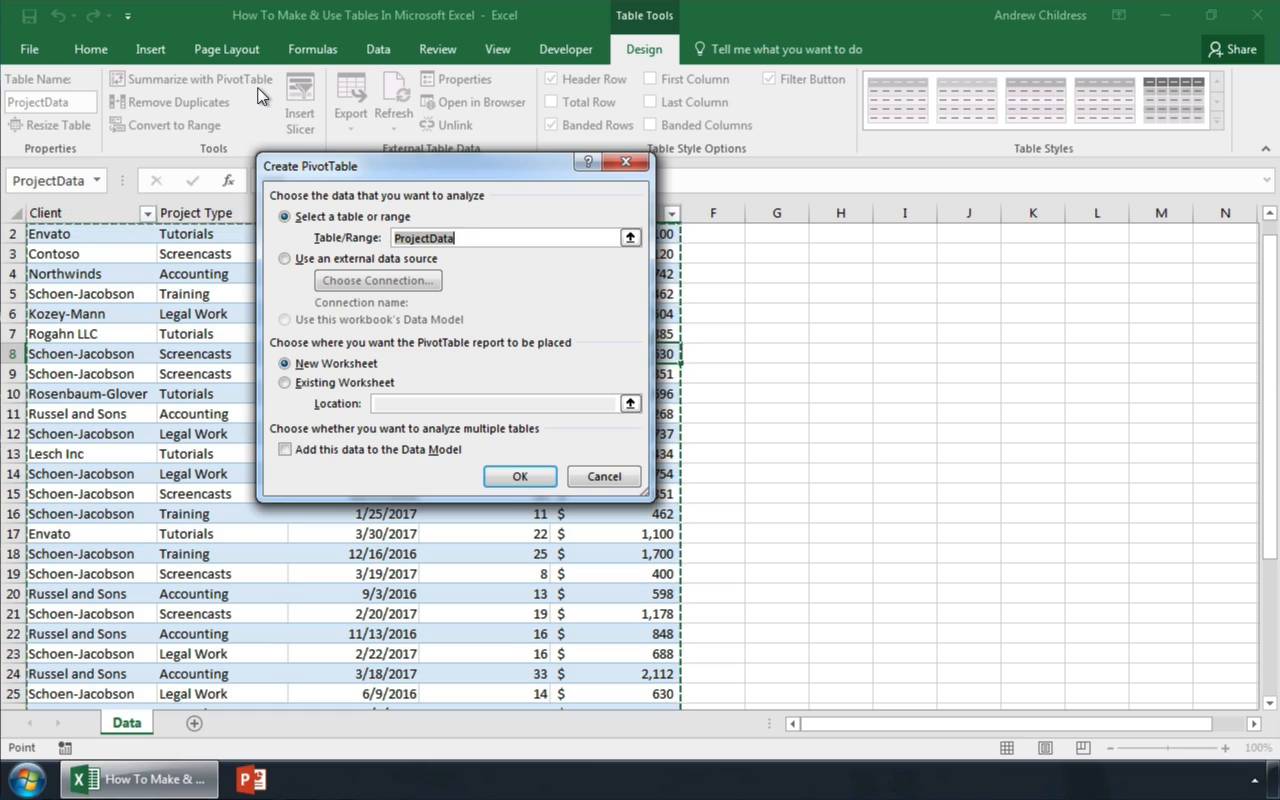
If you want to learn more, keep reading the tutorial below for an illustrated guide to Excel tables.
To follow along with this tutorial, you can use the sample data I’ve included for free in this tutorial. It’s a simple spreadsheet with example data you can use to convert to a table in Excel.
How to Convert Data to a Table in Excel
Here’s how to quickly create a table in Excel:
Start off by clicking inside a set of data in your spreadsheet. You can click anywhere in a set of data before converting it to a table.
Now, you have two choices for how to convert your flat, ordinary data to a table:
- Use the keyboard shortcut, Ctrl + T to convert your data to a table.
- Make sure you’re working on the Home tab on Excel’s ribbon, and click on Format as Table and choose a style (theme) to convert your data to a table.
In either case, you’ll receive this pop-up menu asking you to confirm the table settings:
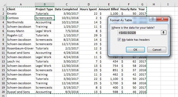


Confirm two settings on this menu:
- Make sure all of your data is selected. You’ll see the green marching ants box around the cells that will be included in your table.
- If your data has headers (titles at the top of the column), leave the My table has headers box checked.
I highly recommend embracing the keyboard shortcut (Ctrl + T) to create tables quickly. When you learn Excel keyboard shortcuts, you’re much more likely to use the feature and embrace it in your own work.
Now that you’ve converted your ordinary data to a table, it’s time to use the power of the feature. Let’s learn more:
How to Use Table Styles in Excel
Tables make it easy to style your data. Instead of spending time highlighting your data, applying background colors and tweaking individual cell styles, tables offer one click styles.
Once you’ve converted your data to a table, click inside of it. A new Excel ribbon option called Table Tools > Design appears on the ribbon.
Click on this ribbon option and find the Table Styles dropdown. Click on one of these style thumbnails to apply the selected color scheme to your data.


Instead of spending time manually styling data, you can use a table to clean up the look of your data. If you only use tables to apply quick styles, it’s still a great feature. But, there’s more you can do with Excel tables:
How to Apply Table Names
One of my favorite table features is the ability to add a name to a table. This makes it easy to reference the table’s data in formulas.
Click inside the table to select it. Then, click on the Design tab on Excel’s ribbon. On the left side of this menu, find the Table Name box and type in a new name for your table. Make sure that it’s a single word (no spaces are allowed in table names.)


Now, you can use the name of the table when you write your formulas. In the example screenshot below, you can see that I’ve pointed a new PivotTable to the table we created in the previous step. Instead of typing out the cell references, I’ve simply typed the name of the table.


Best of all, if the table changes with new rows or columns, these references are smart enough to update as well.
Table names are a must when you create large, robust Excel workbooks. It’s a housekeeping step that ensures you know where your cell references point to.
How to Make Cleaner Excel Formulas
When you write a formula in a table, the formula is more readable and cleaner to review than standard Excel formulas.
In the example below, I’m writing a formula to divide the Amount Billed by the Hours Spent to calculate an Hourly Rate. Notice that the formula that Excel generates isn’t «E2/D2», but instead includes the column names.


Once you press enter, the Excel table will pull the formula down to all of the rows in the table. I prefer the formulas that tables generate when creating calculations. Not only are they cleaner, but you don’t have to pull the formula down manually.
Time-Saving Excel Table Feature: Auto Expand
Tables might evolve over time to include new columns or rows. When you add new data to your tables, they automatically update to include the new columns or rows.
In the example below, you can see an example of what I mean. Once I add a new column in column G and press enter, the table automatically expands and all of the styles are pulled over as well. This means that the table has expanded to include these new columns.


The best part of this feature is that when you’re referencing tables in other formulas, it will automatically include the new rows and columns as well. For example, a PivotTable linked to an Excel data table will update with the new columns and rows when refreshed.
How to Use Excel Table Filters
When you convert data to a table in Excel, you may notice that filter buttons appear at the top of each column. These give you an easy way to restrict the data that appears in the spreadsheet. Click on the dropdown arrow to open the filtering box.
You can check the boxes for the data you want to remove, or uncheck a box to remove it from the table view.


Again, this is a feature that makes using Excel tables worthwhile. You can add filtering without using tables, sure—but with so many features, it makes sense to convert to tables instead.
How to Quickly Apply Subtotals
Subtotals are another great feature that make tables worth using. Turn on totals from the ribbon by clicking on Total Row.


Now, the bottom of each column has a dropdown option to add a total or another math formula. In the last row, click the dropdown arrow to choose an average, total, count, or another math formula.


With this feature, a table becomes a reporting and analysis tool. The subtotals and other figures at the bottom of the table will help you understand your data better.
These subtotals will also adapt if you use filters. For example, if you filter for a single client, the totals will update to only show for that single client.
Recap and Keep Learning More About Excel
It doesn’t matter how much time you spend learning Excel, there’s always more to learn and better ways to use it for controlling your data. Check out these Excel tutorials to keep learning useful spreadsheet skills:
If you haven’t been using tables, are you going to start using them after this tutorial? Let me know in the comments section below.
Did you find this post useful?

I believe that life is too short to do just one thing. In college, I studied Accounting and Finance but continue to scratch my creative itch with my work for Envato Tuts+ and other clients. By day, I enjoy my career in corporate finance, using data and analysis to make decisions.
I cover a variety of topics for Tuts+, including photo editing software like Adobe Lightroom, PowerPoint, Keynote, and more. What I enjoy most is teaching people to use software to solve everyday problems, excel in their career, and complete work efficiently. Feel free to reach out to me on my website.