
Start a new search
To find content from modules and lessons
A collection of cells structured in rows and columns is referred to as a worksheet in Excel documents. It is the work surface that you use to enter data. Each worksheet is a huge table with 1048576 rows and 16384 columns that you may use to organise information.
Sheets in MS Excel are a great way to store data, organize information and create calculations. The sheets tab can be accessed by clicking on the tab at the bottom left of the screen. It will show all the sheets in a workbook and allow you to change their order or delete them.
Sheets and Workbooks are two different types of files in Microsoft Excel. Sheets are the default type of file that’s created when you start a new workbook and they contain one or more worksheets. Workbooks, on the other hand, can contain multiple sheets and other types of files like charts, graphs, or PivotTables.
Sheets in MS Excel offer a lot of advantages. First of all, it is easier to work with them because they are already saved in the cloud. When you make a change to the sheet, it will automatically update for all team members who are working on it. Moreover, you can share your sheets with other people and collaborate on a project easily.
Learner’s Ratings
Reviews
Y
Yash kalra
I dont understood the quiz part the quiz is totally different from the video
S
Sunny kumar
This is a best learning app
K
Kajal Londhe
Best knowledge improve thank you so much
B
Brijesh Yadav
Really thankful to you to explain in such a lucent language
R
RESHMI KUMARI
its very useful for us
S
SHIVAM TIWARI
Formula wala pura uper ja rha
N
Navjeet Kaur
The theory is really good, but practice sheets must also be provided so that we can practice hand to hand. Excel is all about practice more than theory.
A
Aman kesarwani
Hi.
Please mujhe free mai certificate dedo please 😭😥🙏🙏
D
DABLOO Kumar
good and very suficient course
Show More
By clicking the sheet tabs at the bottom of the Excel window, you can quickly select one or more sheets. To enter or edit data on several worksheets at the same time, you can group worksheets by selecting multiple sheets. You can also format or print a selection of sheets at the same time.
|
To select |
Do this |
|---|---|
|
A single sheet |
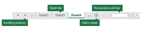
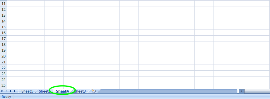
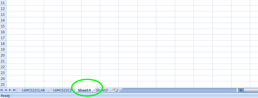
Click the tab for the sheet you want to edit. The active sheet will be a different color than other sheets. In this case, Sheet4 has been selected.
If you don’t see the tab that you want, click the scrolling buttons to locate the tab. You can add a sheet by pressing the Add Sheet button to the right of the sheet tabs. |
|
Two or more adjacent sheets |
Click the tab for the first sheet, then hold down SHIFT while you click the tab for the last sheet that you want to select. By keyboard: First, press F6 to activate the sheet tabs. Next, use the left or right arrow keys to select the sheet you want, then you can use Ctrl+Space to select that sheet. Repeat the arrow and Ctrl+Space steps to select additional sheets. |
|
Two or more nonadjacent sheets |
Click the tab for the first sheet, then hold down CTRL while you click the tabs of the other sheets that you want to select. By keyboard: First, press F6 to activate the sheet tabs. Next, use the left or right arrow keys to select the sheet you want, then you can use Ctrl+Space to select that sheet. Repeat the arrow and Ctrl+Space steps to select additional sheets. |
|
All sheets in a workbook |
Right-click a sheet tab, and then click the Select All Sheets option. |
TIP: After choosing multiple sheets, [Group] appears in the title bar at the top of the worksheet. To cancel a selection of multiple worksheets in a workbook, click any unselected worksheet. If no unselected sheet is visible, right-click the tab of a selected sheet, and then click Ungroup Sheets on the shortcut menu.
NOTES:
-
Data that you enter or edit in the active worksheet will appear in all selected sheets. These changes might replace data on the active sheet and—perhaps unintentionally—on other selected sheets.
-
Data that you copy or cut in grouped sheets cannot be pasted onto another sheet, because the size of the copy area includes all layers of the selected sheets (which is different from the paste area in a single sheet). It’s important to ensure that only one sheet is selected before you copy or move data to another worksheet.
-
When you save a workbook that contains grouped sheets and then close the workbook, the sheets that you selected remain grouped when you reopen that workbook.
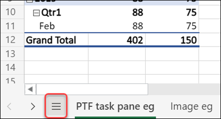
In Excel for the web you can’t select more than one sheet at a time, but it’s easy to find the sheet you want.
-
Select the All Sheets menu, then choose a sheet from the menu to open it.

-
From the sheets listed along the bottom, select a sheet name to open it. Use the arrows just beside the All Sheets menu to scroll forward and backward through sheets to review ones that aren’t currently visible.
A spreadsheet is a grid-based file that organizes data and performs calculations using scalable entries. These are used all over the world to create tables for personal and business purposes. It contains rows and columns of cells and can be used to organize, calculate, and sort data. Spreadsheet data can include text, formulas, references, and functions, as well as numeric values.
A spreadsheet has evolved over the years from a simple grid to a powerful tool that functions as a database or app, performing numerous calculations on one sheet. Using a spreadsheet, you can figure out your mortgage payments over time or determine how depreciation affects your business’s taxes. You can also merge data between several sheets and then visualize it in color-coded tables for better understanding. It can be intimidating for new users to use a spreadsheet program because of all the new features.
A worksheet is a collection of cells(It is a basic data unit in the worksheet), where you can store and manipulate data. By default, every workbook contains at least one worksheet in it. It is easier to organize and locate information in your workbook by using multiple worksheets when working with many data. Adding information to multiple worksheets simultaneously is also easily accomplished by grouping worksheets. In Excel, worksheets can easily be added, renamed, and deleted. Spreadsheet applications like Microsoft Excel are fantastic for maintaining long data lists, budgets, sales figures, etc. A worksheet contains 1048576 rows, 16384 columns, and 17,179,869,184 cells per worksheet.
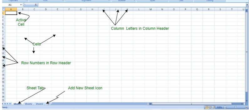
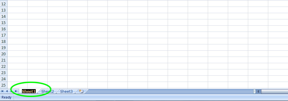
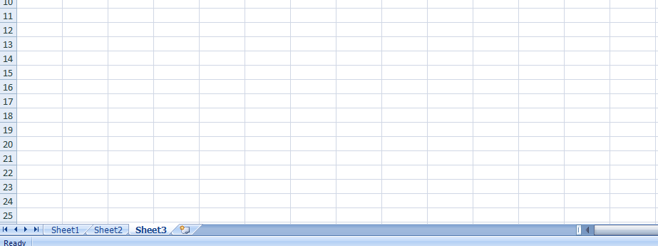
When the Excel program is opened for the first time, the user sees three blank worksheets in the workbook. The screenshot below shows the first worksheet with three tabs at the bottom left corner named Sheet1, Sheet2, and Sheet3. If a workbook contains many worksheets, arrows will also make it easier to view the worksheet tabs.
It is not necessary to delete the two unused worksheets if you’re only using one worksheet – most people don’t bother. Newer versions of Excel save workbooks as xlsx files. Older versions xls extension.
Can we have more than one Excel worksheet in one workbook? According to Microsoft, it’s limited by the number of memory slots on your computer. This is useful if you’re linking data from one worksheet to another, and especially if you’re grouping worksheets that are extremely closely related. However, using the worksheet tabs back and forth can become confusing.
Characteristics of a good worksheet
- An appealing worksheet should have specific titles that indicate what it is about as well as pictures or other clipart to draw some attention.
- It is important that the paper and the writing are in good contrast so that eye strain is minimized.
- Users should be able to do the worksheet independently by following the directions with examples.
- Despite the fact that the worksheet needs to illuminate a pattern in problem solving or usage, it shouldn’t grind an idea into dust.
- Once the worksheet has been completed, the user should be able to explain how it was formed or what it was meant to teach: the answer to this question should be linked to the worksheet’s title.
View a Worksheet
To view a worksheet, click on a worksheet’s tab to view it. Worksheet names and/or many worksheet tabs may not allow the workbook window to display all tabs, so use the arrows on the left of each tab to navigate left or right, or right-click on any arrow and select the worksheet to show from the list.
Click on worksheet to view a worksheet
Rename a Worksheet
To rename a worksheet, follow the following steps:
Step 1: Right-click on the current tab you will get a list.
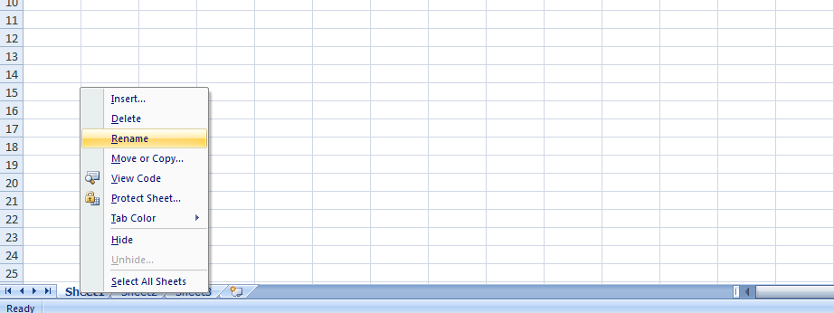
Step 2: Now in this list select Rename option and then typing a new name.
You can also rename the worksheet by double-clicking on the tab.
Insert a Worksheet
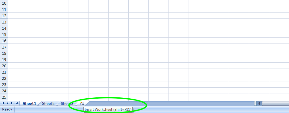
One of the fastest ways to insert a worksheet in a workbook is to click on the small tab to the right of the last worksheet tab. The worksheet can then be moved to a different position if necessary.
Alternative Method to insert a Worksheet
As an alternative, you can add a new worksheet left of an existing worksheet by using the following steps:
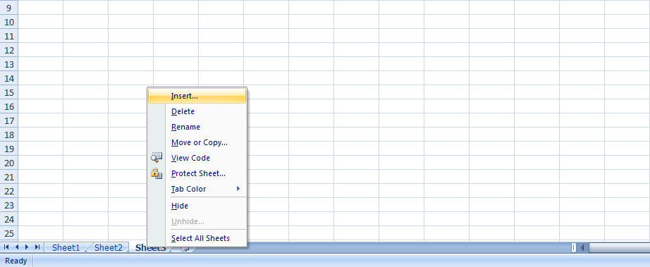
Step 1: Right-click on the tab of the existing worksheet that is just to the right of where you want the new worksheet to be placed. Whenever a spreadsheet is inserted into a worksheet, Excel inserts it to the left.
Step 2: A dialogue box open, here select worksheet.
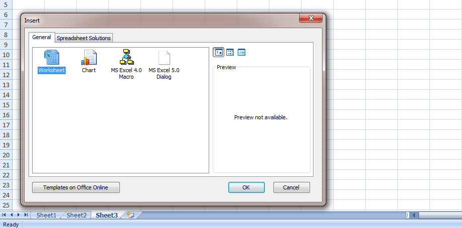
Step 3: Press OK and your new worksheet is add on the left of the current worksheet.
So this is how you can insert new worksheet.
Delete a Worksheet
To delete a worksheet, follow the following steps:
Step 1: Right-click on the current tab(or the tab that your want to delete) you will get a list.
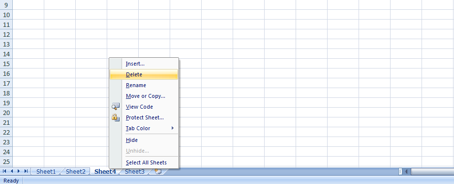
Step 2: Now in this list select the Delete option and your list will be deleted.
So this is how you can delete worksheets.
Example
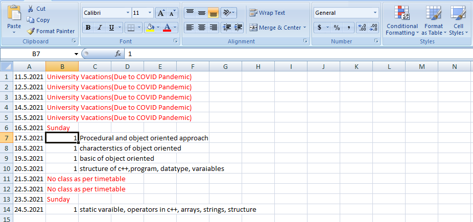
Now, let’s take a working example. Here, I am creating a lesson plan for c++ subject:
Now if I want to teach more than 1 subject then I need to include or insert one more worksheet and for inserting a new worksheet click on the small tab to the right of the last worksheet tab.
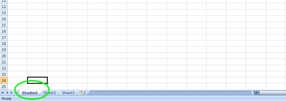
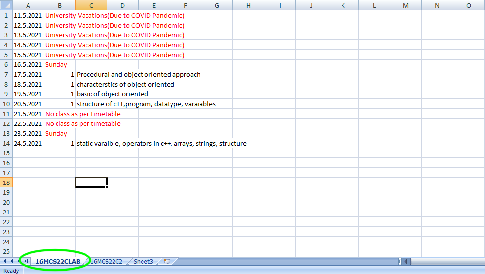
Now, if we want to rename that file then we can rename the spreadsheet tab by right-clicking it, selecting Rename option from the context menu, and then typing a new name. Here, I rename that sheet1 with 16MCS22CLAB.
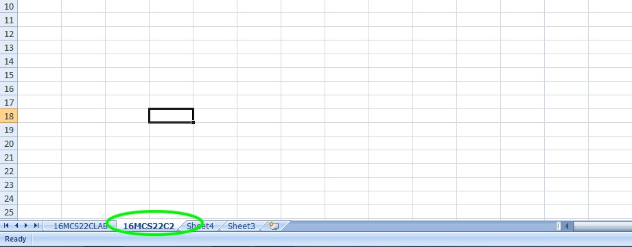
Now, if I want to view the 16MCS22C2 worksheet then click on a worksheet’s tab to view it.
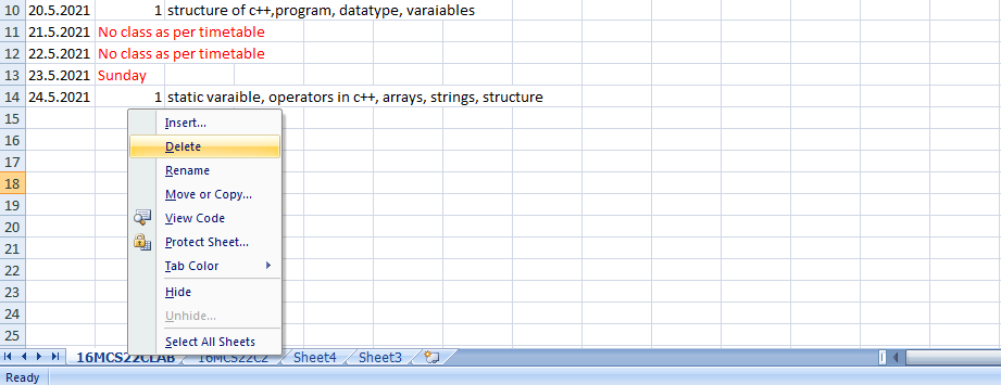
Now, after some time I don’t need the 16MCS22CLAB file. So, to delete that file and for deleting a file, select the Delete option from the context menu by right-clicking the worksheet tab.
Select a Worksheet | Insert a Worksheet | Rename a Worksheet | Move a Worksheet | Delete a Worksheet | Copy a Worksheet | SHEETS function
A worksheet is a collection of cells where you keep and manipulate the data. Each Excel workbook can contain multiple worksheets.
Select a Worksheet
When you open an Excel workbook, Excel automatically selects Sheet1 for you. The name of the worksheet appears on its sheet tab at the bottom of the document window.

Insert a Worksheet
You can insert as many worksheets as you want. To quickly insert a new sheet, click the plus sign at the bottom of the document window.

Result:

Rename a Worksheet
To give a worksheet a more specific name, execute the following steps.
1. Right click on the sheet tab of Sheet1.
2. Choose Rename.

3. For example, type Sales 2016.

Move a Worksheet
To move a worksheet, click on the sheet tab of the worksheet you want to move and drag it into the new position.
1. For example, click on the sheet tab of Sheet2 and drag it before Sales 2016.

Result:

Delete a Worksheet
To delete a worksheet, right click on a sheet tab and choose Delete.
1. For example, delete Sheet2.

Result:

Copy a Worksheet
Imagine, you have got the sales for 2016 ready and want to create the exact same sheet for 2017, but with different data. You can recreate the worksheet, but this is time-consuming. It’s a lot easier to copy the entire worksheet and only change the numbers.
1. Right click on the sheet tab of Sales 2016.
2. Choose Move or Copy.

The ‘Move or Copy’ dialog box appears.
3. Select (move to end) and check Create a copy.

4. Click OK.
Result:

Note: you can even copy a worksheet to another Excel workbook by selecting the specific workbook from the drop-down list (see the dialog box shown earlier).
SHEETS function
To count the total number of worksheets in a workbook, use the SHEETS function in Excel (without any argument).
1. For example, select cell A1.
2. Type =SHEETS() and press Enter.


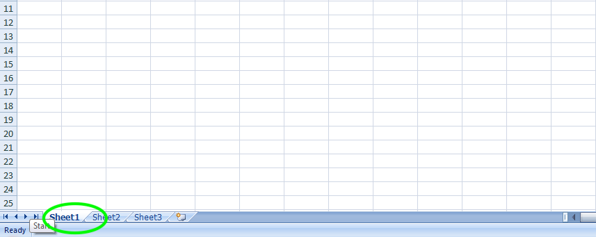
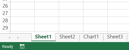
In Microsoft Excel, a sheet is often called a worksheet. A sheet is a single page that contains its own collection of cells to help you organize your data. There can be many sheets in your Excel document and you can see the sheets listed as tabs along the bottom of your document. In this example, we have three sheets in our spreadsheet — Sheet1, Sheet2, and Sheet3.
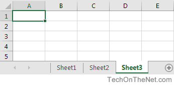
Each sheet has its own name and you can switch between the sheets by clicking on the name of the sheet you want to view. In the example above, we have selected Sheet3.
Traditionally when you create a new Excel document, three sheets (Sheet1, Sheet2, and Sheet3) are created in the spreadsheet and Excel automatically selects Sheet1 for you. In Excel 2016, your spreadsheet will be created with only one sheet called Sheet1. You can then add more sheets as you need them.
There are many things that you can do with sheets in Excel such as inserting, deleting, hiding, unhiding, and renaming sheets. Here is a list of topics that explain how to use sheets in Excel.
Microsoft Office applications are lifesaver for many of us in day-to-day life. Regardless of the education, professional and ethnic background, applications like Excel stand out for decades. Though it is simple to use Excel worksheets to create lists, charts and tables, learning few tips and tricks can save you considerable time. In our earlier article, we have explained about improving productivity in Excel and in this article let us explore tip to manage multiple spreadsheets in Excel workbook.
Related: How to create data validation in Microsoft Excel?
Working with Multiple Worksheets in Excel
Whenever you open an Excel application, it will open a new workbook with a name like “Book1”. Inside a single workbook, you can have multiple sheets for different purposes. You can refer sheets as spreadsheets or worksheets. People work with multiple sheets to prepare a larger output that has inputs spread across sheets. In this kind of scenario, it is essential to effectively manage multiple worksheets in Excel book to get things done quickly.
How to Manage Multiple Spreadsheets in Excel?
Here are few tips and tricks we think can help you in
managing spreadsheets:
- Coloring sheets
- Hide and unhide sheets
- Protect worksheet with password
- Quick reference from another sheet
- Navigating between sheets
- Limit number of sheets
- Naming worksheets properly
- Copy and move worksheets
1. Coloring Worksheets in Excel
By default, all worksheets in a book have same white
background color. When you have multiple worksheets, applying different
background colors to sheets can help you to remember the type of content you
have on each worksheet. You can also use the sheet colors for various other
purposes like keeping all completed task in a green sheet while pending tasks
under yellow or red sheet.
- When you are inside a workbook, right click on the sheet.
- Hover over “Tab Color” and choose the color from the visual color picker tool.

You will see a light background change on the sheet when you
working on it. However, when you move to next sheet, you can see the full
background color for other sheets. You can remove the applied color by again
right clicking and going to “Tab Color > no Color” option.
2. Hide and Unhide Sheets
Probably you already know, you can hide or unhide workbooks from “View > Hide / Unhide” menu. Similar to workbooks, you can also hide or unhide the worksheets to increase the viewability of important sheets on your book.
- Right click on the sheet and select “Hide” option to
hide a sheet. - Use “Control” key to select multiple sheets one by
one. Alternatively, use “Shift” key to select multiple sheets as a block and
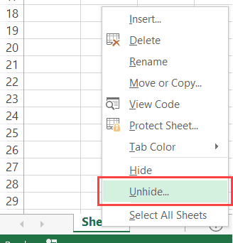
hide them at once. - Similarly, right click and choose “Unhide” to select
the sheet you want to unhide and show.

When you select multiple sheets, Excel will combine them in
single group. You can ungroup from the right click menu or click on any sheet
tab.
Related: How to add and subtract date and time in Excel?
3. Protect Worksheet with Password
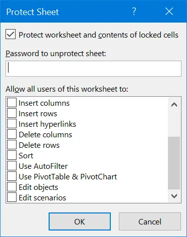
When you do not want anyone to change the content on your sheet, the good idea is to protect or lock the content with a password. The person viewing the sheet will not know the restriction unless he or she tries to edit the cell data. Go to “Review” tab and choose “Protect Sheet” option. Excel will show you a pop-up where you can type a password and select the actions user can do with that sheet.
After saving your workbook, if you or anyone try to modify
the cell data in a protected cell will be prompted with the below message to
enter the password.

Remember not to have sensitive data on your sheet though you
protect, someone can simply delete the entire sheet.
4. Quick Reference from Another Sheet
When you lot of numbers, you may do mathematical calculations from cells referenced across sheets. Though you can go and select the cell for referring, the easy way is to use the text reference. Let us say, you have data in cells B2 and B3 of sheet 1. You can use the below formula, if you want to sum up these two cell data and show in a cell of sheet 2.
=Sheet1!B2+Sheet1!B3
You can click on any cell an apply formula with Sheetx!Cellnumber format for cross reference.
5. Navigating Between Sheets
You can remove the pain of navigating across multiple worksheets by using keyboard shortcuts.
- Control + PageUp to move in left direction
- Control + PageDown move in right direction
6. Limit Number of Sheets
Excel does not restrict the number of sheets in a workbook.
It depends on the available memory size on your computer at that point of time.
We recommend, you to keep the number of sheets within a limit when working with
multiple sheets. Otherwise, you may need to end up in using the small arrows
located in lower left corner.

You can still use Control + Page Up/Down keys to navigate to
next/previous sheet. Alternatively, you can use the following shortcuts.
- Right click on one of the small arrows to select all a
sheet from the pop-up. - Control + Click on left arrow to navigate to first
sheet. - Control + Click on right arrow to navigate to last
sheet.
Note that Excel will remember where you are when closing a
workbook. Next time when you open, it will go to the same sheet when you were
at the time of closing.
Related: How to use VLOOKUP and HLOOKUP in Excel?
7. Naming Worksheets Properly
Excel by default name the worksheets like Sheet1, Sheet 2, etc. This does not make sense when you have multiple sheets with content. You can double click on a sheet or select “Rename” from the right-click context menu to change the name. Having descriptive names will help you to easily navigate and remember the order.

8. Copy, Move and Delete Multiple Worksheets
You can manage moving, deleting and copying worksheets by
right clicking and choosing the appropriate option. Use control or shift keys
to select multiple sheets and delete, move or duplicate them at once.

Remember, in order to move you should drag and drop the
selected sheet(s) in the required position. Excel will show you single or
multiple document icon when you drag. The right click menu only allows you to
move the selected sheet(s) to the end. When you want to copy or duplicate the
entire worksheet, ensure to select “Create a copy” checkbox under “Move or
Copy” pop-up.
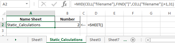
SHEET function is designed to return the number of a specific sheet with a space, which allows access to the entire workbook in MS Excel. SHEETS function provides the user with information on the number of sheets contained in the workbook.
Formulas using links to other Excel sheets
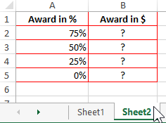
Suppose we have a company DecArt in which employees work and their monthly, salary is calculated. This company has information about the average monthly salary in Excel, and the data on it are placed on different sheets: on sheet 1 there are data on wages, on sheet 2, the percentage bonus. We need to calculate the size of the premium in dollars, while these data were placed on the second sheet.
To begin, consider an example of working with sheets in Excel formulas. Example 1:
- Let’s create on sheet 1 of the workbook of the spreadsheet Excel processor table, as shown in the figure. Information about the average monthly wage:
- Next, on sheet 2 of the workbook, we will prepare an area for placing our result — the size of our premium in dollars, as shown in the figure:
- Next, we will need to enter into the B2 cell the formula shown in the figure below:
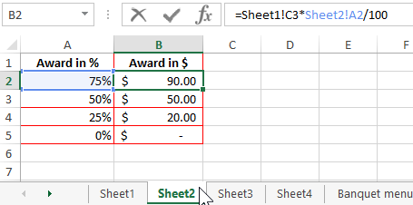
This formula was entered as follows: first, in cell B2, we set the «=» sign, then clicked on «Sheet1» in the lower left corner of the workbook and went to cell C3 on sheet 1, then entered the multiplication operation and switched again to «Sheet2 «to add a percentage.
Thus, when calculating the bonus of each employee, we obtained the initial data on one sheet, and the calculation was made on another sheet. This formula will be very useful when working with longer data sets in large organizations.
SHEETS function to count the number of sheets in a workbook
Consider now the example of the function. It often happens that there are too many sheets in an Excel workbook. It is not possible to visually find out their exact number; it is for this purpose that the SHEETS function has been created.
In this function, only 1 argument — «Link» and even then optional. If it is not filled, then the function returns the total number of sheets created in the current workbook of the Excel file. If necessary, you can fill in the argument. To do this, it is necessary to specify a link to the workbook, in which you need to calculate the total number of sheets created in it.
Example 2. Suppose we have a firm for the production of upholstered furniture, and it has a lot of documents that are contained in the Excel workbook. We need to calculate the exact number of these documents, since each of them has its own name, then it will take time to visually calculate their number.
The figure below shows the approximate number:
To organize the counting of all sheets, you must use function. Simply set the equal sign “=” and enter the function without filling its arguments in brackets. The call to this function is shown below:
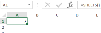
As a result, we obtain the following value: 12 sheets.
Thus, we learned that our company has 12 documents contained in an Excel workbook. This simple example clearly illustrates the operation of the function. This feature can be useful for managers, office workers, sales managers.
Links to other sheets in document templates
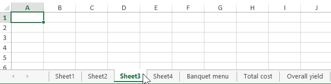
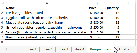
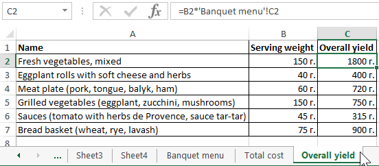
Example 3. There are data on the cost of a banquet company engaged in on-site service. It is necessary to calculate the total cost of the banquet, as well as the total yield of portions of dishes, and calculate the total number of sheets in the document.
- Create a table «Banquet menu», a general view of which is shown in the figure below:
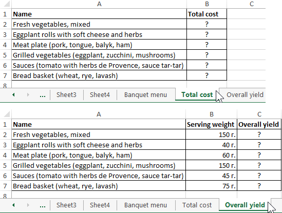
- Similarly, create tables on different sheets «Total cost» and «Total output»:
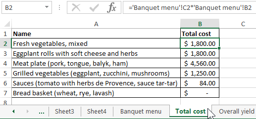
- Using the formula with links to other sheets, we will calculate the total cost of the banquet menu:
- Let’s go to the sheet “Total yield” and by multiplying the cells of the weight of one portion, located on sheet 2 and the total number, located on sheet 1, we will calculate the total output:
See also: Examples of using the SHEET and SHEETS functions in Excel formulas.
Download examples working with other sheets in Excel
As a result, we got the simplest template for calculating the cost of 1 banquet.
На чтение 16 мин. Просмотров 14.8k.

Malcolm Gladwell
Мечтатель начинает с чистого листа бумаги и переосмысливает мир
Эта статья содержит полное руководство по использованию Excel
VBA Worksheet в Excel VBA. Если вы хотите узнать, как что-то сделать быстро, ознакомьтесь с кратким руководством к рабочему листу VBA ниже.
Если вы новичок в VBA, то эта статья — отличное место для начала. Мне нравится разбивать вещи на простые термины и объяснять их на простом языке.
Вы можете прочитать статью от начала до конца, так как она написана в логическом порядке. Или, если предпочитаете, вы можете использовать оглавление ниже и перейти непосредственно к теме по вашему выбору.
Содержание
- Краткое руководство к рабочему листу VBA
- Вступление
- Доступ к рабочему листу
- Использование индекса для доступа к рабочему листу
- Использование кодового имени рабочего листа
- Активный лист
- Объявление объекта листа
- Доступ к рабочему листу в двух словах
- Добавить рабочий лист
- Удалить рабочий лист
- Цикл по рабочим листам
- Использование коллекции листов
- Заключение
Краткое руководство к рабочему листу VBA
В следующей таблице приведен краткий обзор различных методов
Worksheet .
Примечание. Я использую Worksheet в таблице ниже, не указывая рабочую книгу, т.е. Worksheets, а не ThisWorkbook.Worksheets, wk.Worksheets и т.д. Это сделано для того, чтобы примеры были понятными и удобными для чтения. Вы должны всегда указывать рабочую книгу при использовании Worksheets . В противном случае активная рабочая книга будет использоваться по умолчанию.
| Задача | Исполнение |
| Доступ к рабочему листу по имени |
Worksheets(«Лист1») |
| Доступ к рабочему листу по позиции слева |
Worksheets(2) Worksheets(4) |
| Получите доступ к самому левому рабочему листу |
Worksheets(1) |
| Получите доступ к самому правому листу |
Worksheets(Worksheets.Count) |
| Доступ с использованием кодового имени листа (только текущая книга) |
Смотри раздел статьи Использование кодового имени |
| Доступ по кодовому имени рабочего листа (другая рабочая книга) |
Смотри раздел статьи Использование кодового имени |
| Доступ к активному листу | ActiveSheet |
| Объявить переменную листа | Dim sh As Worksheet |
| Назначить переменную листа | Set sh = Worksheets(«Лист1») |
| Добавить лист | Worksheets.Add |
| Добавить рабочий лист и назначить переменную |
Worksheets.Add Before:= Worksheets(1) |
| Добавить лист в первую позицию (слева) |
Set sh =Worksheets.Add |
| Добавить лист в последнюю позицию (справа) |
Worksheets.Add after:=Worksheets(Worksheets.Count) |
| Добавить несколько листов | Worksheets.Add Count:=3 |
| Активировать рабочий лист | sh.Activate |
| Копировать лист | sh.Copy |
| Копировать после листа | sh1.Copy After:=Sh2 |
| Скопировать перед листом | sh1.Copy Before:=Sh2 |
| Удалить рабочий лист | sh.Delete |
| Удалить рабочий лист без предупреждения |
Application.DisplayAlerts = False sh.Delete Application.DisplayAlerts = True |
| Изменить имя листа | sh.Name = «Data» |
| Показать/скрыть лист | sh.Visible = xlSheetHidden sh.Visible = xlSheetVisible sh.Name = «Data» |
| Перебрать все листы (For) | Dim i As Long For i = 1 To Worksheets.Count Debug.Print Worksheets(i).Name Next i |
| Перебрать все листы (For Each) | Dim sh As Worksheet For Each sh In Worksheets Debug.Print sh.Name Next |
Вступление
Три наиболее важных элемента VBA — это Рабочая книга, Рабочий лист и Ячейки. Из всего кода, который вы пишете, 90% будут включать один или все из них.
Наиболее распространенное использование Worksheet в VBA для доступа к его ячейкам. Вы можете использовать его для защиты, скрытия, добавления, перемещения или копирования листа.
Тем не менее, вы будете в основном использовать его для выполнения некоторых действий с одной или несколькими ячейками на листе.
Использование Worksheets более простое, чем использование рабочих книг. С книгами вам может потребоваться открыть их, найти, в какой папке они находятся, проверить, используются ли они, и так далее. С рабочим листом он либо существует в рабочей книге, либо его нет.
Доступ к рабочему листу
В VBA каждая рабочая книга имеет коллекцию рабочих листов. В этой коллекции есть запись для каждого рабочего листа. Эта коллекция называется просто Worksheets и используется очень похоже на коллекцию Workbooks. Чтобы получить доступ к рабочему листу, достаточно указать имя.
Приведенный ниже код записывает «Привет Мир» в ячейках A1 на листах: Лист1, Лист2 и Лист3 текущей рабочей книги.
Sub ZapisVYacheiku1()

    ' Запись в ячейку А1 в листе 1, листе 2 и листе 3
    ThisWorkbook.Worksheets("Лист1").Range("A1") = "Привет Мир"
    ThisWorkbook.Worksheets("Лист2").Range("A1") = "Привет Мир"
    ThisWorkbook.Worksheets("Лист3").Range("A1") = "Привет Мир"

End Sub
Коллекция Worksheets всегда принадлежит книге. Если мы не
указываем рабочую книгу, то активная рабочая книга используется по умолчанию.
Sub ZapisVYacheiku1()

    ' Worksheets относятся к рабочим листам в активной рабочей книге.
    Worksheets("Лист1").Range("A1") = "Привет Мир"
    Worksheets("Лист2").Range("A1") = "Привет Мир"
    Worksheets("Лист3").Range("A1") = "Привет Мир"

End Sub
Скрыть рабочий лист
В следующих примерах показано, как скрыть и показать лист.
ThisWorkbook.Worksheets("Лист1").Visible = xlSheetHidden

ThisWorkbook.Worksheets("Лист1").Visible = xlSheetVisible
Если вы хотите запретить пользователю доступ к рабочему
листу, вы можете сделать его «очень скрытым». Это означает, что это может быть
сделано видимым только кодом.
' Скрыть от доступа пользователя
ThisWorkbook.Worksheets("Лист1").Visible = xlVeryHidden

' Это единственный способ сделать лист xlVeryHidden видимым
ThisWorkbook.Worksheets("Лист1").Visible = xlSheetVisible
Защитить рабочий лист
Другой пример использования Worksheet — когда вы хотите защитить его.
ThisWorkbook.Worksheets("Лист1").Protect Password:="Мойпароль"

ThisWorkbook.Worksheets("Лист1").Unprotect Password:="Мойпароль"
Индекс вне диапазона
При использовании Worksheets вы можете получить сообщение об
ошибке:
Run-time Error 9 Subscript out of Range

Это означает, что вы пытались получить доступ к рабочему листу, который не существует. Это может произойти по следующим причинам:
- Имя Worksheet , присвоенное рабочим листам, написано неправильно.
- Название листа изменилось.
- Рабочий лист был удален.
- Индекс был большим, например Вы использовали рабочие листы (5), но есть только четыре рабочих листа
- Используется неправильная рабочая книга, например Workbooks(«book1.xlsx»).Worksheets(«Лист1») вместо
Workbooks(«book3.xlsx»).Worksheets («Лист1»).
Если у вас остались проблемы, используйте один из циклов из раздела «Циклы по рабочим листам», чтобы напечатать имена всех рабочих листов коллекции.
Использование индекса для доступа к рабочему листу
До сих пор мы использовали имя листа для доступа к листу.
Указатель относится к положению вкладки листа в рабочей книге. Поскольку
положение может быть легко изменено пользователем, не рекомендуется
использовать это.
В следующем коде показаны примеры использования индекса.
' Использование этого кода является плохой идеей, так как
' позиции листа все время меняются
Sub IspIndList()

    With ThisWorkbook
        ' Самый левый лист
        Debug.Print .Worksheets(1).Name
        ' Третий лист слева
        Debug.Print .Worksheets(3).Name
        ' Самый правый лист
        Debug.Print .Worksheets(.Worksheets.Count).Name
    End With

End Sub
В приведенном выше примере я использовал Debug.Print для печати в Immediate Window. Для просмотра этого окна выберите «Вид» -> «Immediate Window » (Ctrl + G).


Использование кодового имени рабочего листа
Лучший способ получить доступ к рабочему листу —
использовать кодовое имя. Каждый лист имеет имя листа и кодовое имя. Имя листа
— это имя, которое отображается на вкладке листа в Excel.
Изменение имени листа не приводит к изменению кодового имени, что означает, что ссылка на лист по кодовому имени — отличная идея.
Если вы посмотрите в окне свойств VBE, вы увидите оба имени.
На рисунке вы можете видеть, что кодовое имя — это имя вне скобок, а имя листа
— в скобках.

Вы можете изменить как имя листа, так и кодовое имя в окне
свойств листа (см. Изображение ниже).

Если ваш код ссылается на кодовое имя, то пользователь может
изменить имя листа, и это не повлияет на ваш код. В приведенном ниже примере мы
ссылаемся на рабочий лист напрямую, используя кодовое имя.
Sub IspKodImya2()

    ' Используя кодовое имя листа
    Debug.Print CodeName.Name
    CodeName.Range("A1") = 45
    CodeName.Visible = True

End Sub
Это делает код легким для чтения и безопасным от изменения
пользователем имени листа.
Кодовое имя в других книгах
Есть один недостаток использования кодового имени. Он относится только к рабочим листам в рабочей книге, которая содержит код, т.е. ThisWorkbook.
Однако мы можем использовать простую функцию, чтобы найти
кодовое имя листа в другой книге.
Sub ИспЛист()

    Dim sh As Worksheet
    ' Получить рабочий лист под кодовым именем
    Set sh = SheetFromCodeName("CodeName", ThisWorkbook)
    ' Используйте рабочий лист
    Debug.Print sh.Name

End Sub

' Эта функция получает объект листа из кодового имени
Public Function SheetFromCodeName(Name As String, bk As Workbook) As Worksheet

    Dim sh As Worksheet
    For Each sh In bk.Worksheets
        If sh.CodeName = Name Then
           Set SheetFromCodeName = sh
           Exit For
        End If
    Next sh

End Function
Использование приведенного выше кода означает, что если
пользователь изменит имя рабочего листа, то на ваш код это не повлияет.
Существует другой способ получения имени листа внешней
рабочей книги с использованием кодового имени. Вы можете использовать элемент
VBProject этой Рабочей книги.
Вы можете увидеть, как это сделать, в примере ниже. Я включил это, как дополнительную информацию, я бы рекомендовал использовать метод из предыдущего примера, а не этот.
Public Function SheetFromCodeName2(codeName As String _
                             , bk As Workbook) As Worksheet

    ' Получить имя листа из CodeName, используя VBProject
    Dim sheetName As String
    sheetName = bk.VBProject.VBComponents(codeName).Properties("Name")

    ' Используйте имя листа, чтобы получить объект листа
    Set SheetFromCodeName2 = bk.Worksheets(sheetName)

End Function
Резюме кодового имени
Ниже приведено краткое описание использования кодового имени:
- Кодовое имя рабочего листа может быть
использовано непосредственно в коде, например. Sheet1.Range - Кодовое имя будет по-прежнему работать, если имя
рабочего листа будет изменено. - Кодовое имя может использоваться только для
листов в той же книге, что и код. - Везде, где вы видите ThisWorkbook.Worksheets
(«имя листа»), вы можете заменить его кодовым именем рабочего листа. - Вы можете использовать функцию SheetFromCodeName
сверху, чтобы получить кодовое имя рабочих листов в других рабочих книгах.
Активный лист
Объект ActiveSheet ссылается на рабочий лист, который в данный момент активен. Вы должны использовать ActiveSheet только в том случае, если у вас есть особая необходимость ссылаться на активный лист.
В противном случае вы должны указать рабочий лист, который
вы используете.
Если вы используете метод листа, такой как Range, и не
упоминаете лист, он по умолчанию будет использовать активный лист.
' Написать в ячейку A1 в активном листе
ActiveSheet.Range("A1") = 99

' Активный лист используется по умолчанию, если лист не используется
Range("A1") = 99
Объявление объекта листа
Объявление объекта листа полезно для того, чтобы сделать ваш
код более понятным и легким для чтения.
В следующем примере показан код для обновления диапазонов
ячеек. Первый Sub не объявляет объект листа. Вторая подпрограмма объявляет
объект листа, и поэтому код намного понятнее.
Sub NeObyavObektList()

    Debug.Print ThisWorkbook.Worksheets("Лист1").Name
    ThisWorkbook.Worksheets("Лист1").Range("A1") = 6
    ThisWorkbook.Worksheets("Лист1").Range("B2:B9").Font.Italic = True
    ThisWorkbook.Worksheets("Лист1").Range("B2:B9").Interior.Color = rgbRed

End Sub
Sub ObyavObektList()

    Dim sht As Worksheet
    Set sht = ThisWorkbook.Worksheets("Лист1")

    sht.Range("A1") = 6
    sht.Range("B2:B9").Font.Italic = True
    sht.Range("B2:B9").Interior.Color = rgbRed

End Sub
Вы также можете использовать ключевое слово With с объектом
листа, как показано в следующем примере.
Sub ObyavObektListWith()

    Dim sht As Worksheet
    Set sht = ThisWorkbook.Worksheets("Лист1")

    With sht
        .Range("A1") = 6
        .Range("B2:B9").Font.Italic = True
        .Range("B2:B9").Interior.Color = rgbRed
    End With

End Sub
Доступ к рабочему листу в двух словах
Из-за множества различных способов доступа к рабочему листу вы можете быть сбитыми с толку. Так что в этом разделе я собираюсь разбить его на простые термины.
- Если вы хотите использовать тот лист, который активен в данный момент, используйте ActiveSheet.
ActiveSheet.Range("A1") = 55
2. Если лист находится в той же книге, что и код, используйте кодовое имя.
3. Если рабочая таблица находится в другой рабочей книге, сначала получите рабочую книгу, а затем получите рабочую таблицу.
' Получить рабочую книгу
Dim wk As Workbook
Set wk = Workbooks.Open("C:ДокументыСчета.xlsx", ReadOnly:=True)
' Затем получите лист
Dim sh As Worksheet
Set sh = wk.Worksheets("Лист1")
Если вы хотите защитить пользователя от изменения имени листа, используйте функцию SheetFromCodeName из раздела «Имя кода».
' Получить рабочую книгу
Dim wk As Workbook
Set wk = Workbooks.Open("C:ДокументыСчета.xlsx", ReadOnly:=True)

' Затем получите лист
Dim sh As Worksheet
Set sh = SheetFromCodeName("sheetcodename",wk)
Добавить рабочий лист
Примеры в этом разделе показывают, как добавить новую
рабочую таблицу в рабочую книгу. Если вы не предоставите никаких аргументов для
функции Add, то новый
рабочий лист будет помещен перед активным рабочим листом.
Когда вы добавляете рабочий лист, он создается с именем по умолчанию, например «Лист4». Если вы хотите изменить имя, вы можете легко сделать это, используя свойство Name.
В следующем примере добавляется новый рабочий лист и изменяется имя на «Счета». Если лист с именем «Счета» уже существует, вы получите сообщение об ошибке.
Sub DobavitList()

    Dim sht As Worksheet

    ' Добавляет новый лист перед активным листом
    Set sht = ThisWorkbook.Worksheets.Add
    ' Установите название листа
    sht.Name = "Счета"

    ' Добавляет 3 новых листа перед активным листом
    ThisWorkbook.Worksheets.Add Count:=3

End Sub
В предыдущем примере вы добавляете листы по отношению к
активному листу. Вы также можете указать точную позицию для размещения листа.
Для этого вам нужно указать, какой лист новый лист должен
быть вставлен до или после. Следующий код показывает вам, как это сделать.
Sub DobavitListPervPosl()

    Dim shtNew As Worksheet
    Dim shtFirst As Worksheet, shtLast As Worksheet

    With ThisWorkbook

        Set shtFirst = .Worksheets(1)
        Set shtLast = .Worksheets(.Worksheets.Count)

        ' Добавляет новый лист на первую позицию в книге
        Set shtNew = Worksheets.Add(Before:=shtFirst)
        shtNew.Name = "FirstSheet"

        ' Добавляет новый лист к последней позиции в книге
        Set shtNew = Worksheets.Add(After:=shtLast)
        shtNew.Name = "LastSheet"

    End With

End Sub
Удалить рабочий лист
Чтобы удалить лист, просто вызовите Delete.
Dim sh As Worksheet
Set sh = ThisWorkbook.Worksheets("Лист12")
sh.Delete
Excel отобразит предупреждающее сообщение при удалении листа. Если вы хотите скрыть это сообщение, вы можете использовать код ниже:
Application.DisplayAlerts = False
sh.Delete
Application.DisplayAlerts = True
Есть два аспекта, которые нужно учитывать при удалении таблиц.
Если вы попытаетесь получить доступ к рабочему листу после
его удаления, вы получите ошибку «Subscript out of Range», которую мы видели в
разделе «Доступ к рабочему листу».
Dim sh As Worksheet
Set sh = ThisWorkbook.Worksheets("Лист2")
sh.Delete

' Эта строка выдаст «Subscript out of Range», так как «Лист2» не существует
Set sh = ThisWorkbook.Worksheets("Лист2")
Вторая проблема — когда вы назначаете переменную листа. Если вы попытаетесь использовать эту переменную после удаления листа, вы получите ошибку автоматизации, подобную этой:
Run-Time error -21147221080 (800401a8′) Automation Error
Если вы используете кодовое имя рабочего листа, а не
переменную, это приведет к сбою Excel,
а не к ошибке автоматизации.
В следующем примере показано, как происходят ошибки автоматизации.
sh.Delete

' Эта строка выдаст ошибку автоматизации
Debug.Assert sh.Name
Если вы назначите переменную Worksheet действительному рабочему листу, он будет работать нормально.
sh.Delete

' Назначить sh на другой лист
Set sh = Worksheets("Лист3")

' Эта строка будет работать нормально
Debug.Assert sh.Name
Цикл по рабочим листам
Элемент «Worksheets» — это набор рабочих листов, принадлежащих рабочей книге. Вы можете просмотреть каждый лист в коллекции рабочих листов, используя циклы «For Each» или «For».
В следующем примере используется цикл For Each.
Sub CiklForEach()

    ' Записывает «Привет Мир» в ячейку A1 для каждого листа
    Dim sht As Worksheet
    For Each sht In ThisWorkbook.Worksheets
         sht.Range("A1") = "Привет Мир"
    Next sht

End Sub
В следующем примере используется стандартный цикл For.
Sub CiklFor()

    ' Записывает «Привет Мир» в ячейку A1 для каждого листа
    Dim i As Long
    For i = 1 To ThisWorkbook.Worksheets.Count
         ThisWorkbook.Worksheets(i).Range("A1") = "Привет Мир"
    Next sht

End Sub
Вы видели, как получить доступ ко всем открытым рабочим книгам и как получить доступ ко всем рабочим листам в ThisWorkbook. Давайте сделаем еще один шаг вперед — узнаем, как получить доступ ко всем рабочим листам во всех открытых рабочих книгах.
Примечание. Если вы используете код, подобный этому, для записи на листы, то сначала сделайте резервную копию всего, так как в итоге вы можете записать неверные данные на все листы.
Sub NazvVsehStr()

    ' Печатает рабочую книгу и названия листов для
    ' всех листов в открытых рабочих книгах
    Dim wrk As Workbook
    Dim sht As Worksheet
    For Each wrk In Workbooks
        For Each sht In wrk.Worksheets
            Debug.Print wrk.Name + ":" + sht.Name
        Next sht
    Next wrk

End Sub
Использование коллекции листов
Рабочая книга имеет еще одну коллекцию, похожую на Worksheets под названием Sheets. Это иногда путает пользователей. Чтобы понять, в первую очередь, вам нужно знать о типе листа, который является диаграммой.
В Excel есть возможность создать лист, который является диаграммой. Для этого нужно:
- Создать диаграмму на любом листе.
- Щелкнуть правой кнопкой мыши на графике и выбрать «Переместить».
- Выбрать первый вариант «Новый лист» и нажмите «ОК».
Теперь у вас есть рабочая книга, в которой есть типовые листы и лист-диаграмма.
- Коллекция «Worksheets » относится ко всем рабочим листам в рабочей книге. Не включает в себя листы типа диаграммы.
- Коллекция Sheets относится ко всем листам, принадлежащим книге, включая листы типовой диаграммы.
Ниже приведены два примера кода. Первый проходит через все
листы в рабочей книге и печатает название листа и тип листа. Второй пример
делает то же самое с коллекцией Worksheets.
Чтобы опробовать эти примеры, вы должны сначала добавить лист-диаграмму в свою книгу, чтобы увидеть разницу.
Sub KollSheets()

    Dim sht As Variant
    ' Показать название и тип каждого листа
    For Each sht In ThisWorkbook.Sheets
        Debug.Print sht.Name & " is type " & TypeName(sht)
    Next sht

End Sub

Sub KollWorkSheets()

    Dim sht As Variant
    ' Показать название и тип каждого листа
    For Each sht In ThisWorkbook.Worksheets
        Debug.Print sht.Name & " is type " & TypeName(sht)
    Next sht

End Sub
Если у вас нет листов диаграмм, то использование коллекции Sheets — то же самое, что использование коллекции WorkSheets.
Заключение
На этом мы завершаем статью о Worksheet VBA. Я надеюсь, что было полезным.
Три наиболее важных элемента Excel VBA — это рабочие книги, рабочие таблицы, диапазоны и ячейки.
Эти элементы будут использоваться практически во всем, что вы делаете. Понимание их сделает вашу жизнь намного проще и сделает изучение VBA увлекательнее.
How To Use Excel:
A Beginner’s Guide To Getting Started
Written by co-founder Kasper Langmann, Microsoft Office Specialist.
Excel is a powerful application—but it can also be very intimidating.
That’s why we’ve put together this beginner’s guide to getting started with Excel.
It will take you from the very beginning (opening a spreadsheet), through entering and working with data, and finish with saving and sharing.
It’s everything you need to know to get started with Excel.
If you want to tag along as you read, please download the free sample Excel workbook here.
Opening an Excel spreadsheet
When you first open Excel (by double-clicking the icon or selecting it from the Start menu), the application will ask what you want to do.

If you want to open a new Excel spreadsheet, click Blank workbook.
To open an existing spreadsheet (like the example workbook you just downloaded), click Open Other Workbooks in the lower-left corner, then click Browse on the left side of the resulting window.

Then use the file explorer to find the Excel workbook you’re looking for, select it, and click Open.
Workbooks vs. spreadsheets
There’s something we should clear up before we move on.
A workbook is an Excel file. It usually has a file extension of .XLSX (if you’re using an older version of Excel, it could be .XLS).
A spreadsheet is a single sheet inside a workbook. There can be many sheets inside of a workbook, and they’re accessed via the tabs at the bottom of the screen.
A spreadsheet (a.k.a. a sheet/tab) contains all the cells you can see and use in the >1 million rows >16,000 columns.
Working with the Ribbon
The Ribbon is the central control panel of Excel. You can do just about everything you need to directly from the Ribbon.
Where is this powerful tool? At the top of the window:

There are a number of tabs, including the File tab, Home tab, Insert tab, Data tab, Review tab, and a few others. Each tab contains different buttons.
Try clicking on a few different tabs to see which buttons appear below them.
 Kasper Langmann, Co-founder of Spreadsheeto
There’s also a very useful search bar in the Ribbon. It says Tell me what you want to do. Just type in what you’re looking for, and Excel will help you find it.

Most of the time, you’ll be in the Home tab of the Ribbon. But Formulas and Data are also very useful (we’ll be talking about formulas shortly).
Pro tip: Ribbon sections
In addition to tabs, the Ribbon also has some smaller sections. And when you’re looking for something specific, those sections can help you find it.
For example, if you’re looking for sorting and filtering options, you don’t want to hover over dozens of buttons finding out what they do.
Instead, skim through the section names until you find what you’re looking for:

Managing your sheets
As we saw, workbooks can contain multiple sheets.
You can manage those sheets with the sheet tabs near the bottom of the screen. Click a tab to open that particular worksheet.
If you’re using our example workbook, you’ll see two sheets, called Welcome and Thank You:

To add a new worksheet, click the + (plus) button at the end of the list of sheets.
You can also reorder the sheets in your workbook by dragging them to a new location.
And if you right-click a worksheet tab, you’ll get a number of options:

For now, don’t worry too much about these options. Rename and Delete are useful, but the rest needn’t concern you.
Kasper Langmann, Co-founder of SpreadsheetoEntering data
Now it’s time to enter some data!
And while entering data is one of the most central and important things you can do in Excel, it’s almost effortless.
Just click into a blank cell and start typing.
Go ahead, try it! Type your name, birthday, and your favorite number into some blank cells.
Kasper Langmann, Co-founder of SpreadsheetoYou can also copy (Ctrl + C), cut (Ctrl + X), and paste (Ctrl + V) any data you’d like (or read our full guide on copying and pasting here).
Try copying and pasting the data from multiple cells inthe example spreadsheet into another column.
You can also copy data from other programs into Excel.
Try copying this list of numbers and pasting it into your sheet:
- 17
- 24
- 9
- 00
- 3
- 12
That’s all we’re going to cover for basic data entry. Just know that there are lots of other ways to get data into your spreadsheets if you need them.
Kasper Langmann, Co-founder of SpreadsheetoBasic calculations
Now that we’ve seen how to get some basic data into our spreadsheet, we’re going to do some things with it.
Running basic calculations in Excel is easy. First, we’ll look at how to add two numbers.
Important: start calculations with = (equals)
When you’re running a calculation (or a formula, which we’ll discuss next), the first thing you need to type is an equals sign. This tells Excel to get ready to run some sort of calculation.
So when you see something like =MEDIAN(A2:A51), make sure you type it exactly as it is—including the equals sign.
Let’s add 3 and 4. Type the following formula in a blank cell:
=3+4
Then hit Enter.

When you hit Enter, Excel evaluates your equation and displays the result, 7.
But if you look above at the formula bar, you’ll still see the original formula.
That’s a useful thing to keep in mind, in case you forget what you typed originally.
You can also edit a cell in the formula bar. Click on any cell, then click into the formula bar and start typing.
Kasper Langmann, Co-founder of SpreadsheetoPerforming subtraction, multiplication, and division is just as easy. Try these formulas:
- =4-6
- =2*5
- =-10/3
What we’re going to cover next is one of the most important things in Excel. We’re giving it a very basic overview here, but feel free to read our post on cell references to get the details.
Kasper Langmann, Co-founder of SpreadsheetoNow let’s try something different. Open up the first sheet in the example workbook, click into cell C1, and type the following:
=A1+B1
Hit Enter.
You should get 82, the sum of the numbers in cells A1 and B1.
Now, change one of the numbers in A1 or B1 and watch what happens:
Because you’re adding A1 and B1, Excel automatically updates the total when you change the values in one of those cells.
Try doing different types of arithmetic on the other numbers in columns A and B using this method.
Unlocking the power of functions
Excel’s greatest power lies in functions. These let you run complex calculations with a few keypresses.
We’ll barely scratch the surface of functions here. Check out our other blog posts to see some of the great things you can do with functions!
Kasper Langmann, Co-founder of SpreadsheetoMany formulas take sets of numbers and give you information about them.
For example, the AVERAGE function gives you the average of a set of numbers. Let’s try using it.
Click into an empty cell and type the following formula:
=AVERAGE(A1:A4)
Then hit Enter.

The resulting number, 0.25, is the average of the numbers in cells A1, A2, A3, and A4.
Cell range notation
In the formula above, we used “A1:A4” to tell Excel to look at all the cells between A1 and A4, including both of those cells. You can read it as “A1 through A4.”
You can also use this to include numbers in different columns. “A5:C7” includes A5, A6, A7, B5, B6, B7, C5, C6, and C7.
There are also functions that work on text.
Let’s try the CONCATENATE function!
Click into cell C5 and type this formula:
=CONCATENATE(A5, ” “, B5)
Then hit Enter.
You’ll see the message “Welcome to Spreadsheeto” in the cell.
How did this happen? CONCATENATE takes cells with text in them and puts them together.
We put the contents of A5 and B5 together. But because we also needed a space between “to” and “Spreadsheeto,” we included a third argument: the space between two quotes.
Remember that you can mix cell references (like “A5″) and typed values (like ” “) in formulas.
Kasper Langmann, Co-founder of SpreadsheetoExcel has dozens of useful functions. To find the function that will solve a particular problem, head to the Formulas tab and click on one of the icons:

Scroll through the list of available functions, and select the one you want (you may have to look around for a while).
Then Excel will help you get the right numbers in the right places:

If you start typing a formula, starting with the equals sign, Excel will help you by showing you some possible functions that you might be looking for:

And finally, once you’ve typed the name of a formula and the opening parenthesis, Excel will tell you which arguments need to go where:

If you’ve never used a function before, it might be difficult to interpret Excel’s reminders. But once you get more experience, it’ll become clear.
This is a tiny preview of how functions work and what they can do. It should be enough to get you going on the tasks you need to accomplish right away.
Kasper Langmann, Co-founder of SpreadsheetoSaving and sharing your work
After you’ve done a bunch of work with your spreadsheet, you’re going to want to save your changes.
Hit Ctrl + S to save. If you haven’t yet saved your spreadsheet, you’ll be asked where you want to save it and what you want to call it.
You can also click the Save button in the Quick Access Toolbar:

It’s a good idea to get into the habit of saving often. Trying to recover unsaved changes is a pain!
Kasper Langmann, Co-founder of SpreadsheetoThe easiest way to share your spreadsheets is via OneDrive.
Click the Share button in the top-right corner of the window, and Excel will walk you through sharing your document.

You can also save your document and email it, or use any other cloud service to share it with others.
That’s it – Now what?
This was how to use Excel.
Or… at least a small fraction of it.
Microsoft Excel can be intimidating, but once you get the basics down, it’s easier to learn the more advanced functions.
This was your introduction to “the basics”. So, if you’re not ready to get some advanced Excel knowledge, go ahead and practice with some of the existing data at the office 🧑🏼💻
If you’re ready to take your next steps, go ahead and enroll in my 30-minute free online course where you learn: IF, SUMIF, VLOOKUP, and data cleaning.
These are some of the most important topics of Excel💪🏼
Other resources
Now, you can’t excel at Excel without mastering some of the lookup functions like VLOOKUP and the new XLOOKUP.
But also, you don’t wanna miss out on pivot tables. You can use these to transform your Microsoft Excel data into insightful reports in just a few clicks🤯
Or if you’re into automating Excel spreadsheet formatting, go ahead and read my guide to conditional formatting here.
Kasper Langmann2023-02-23T14:45:07+00:00
Page load link
Apart from cells and ranges, working with worksheets is another area you should know about to use VBA efficiently in Excel.
Just like any object in VBA, worksheets have different properties and methods associated with it that you can use while automating your work with VBA in Excel.
In this tutorial, I will cover ‘Worksheets’ in detail and also show you some practical examples.
So let’s get started.
All the codes I mention in this tutorial need to be placed in the VB Editor. Go to the ‘Where to Put the VBA Code‘ section to know how it works.
If you’re interested in learning VBA the easy way, check out my Online Excel VBA Training.
Difference between Worksheets and Sheets in VBA
In VBA, you have two collections that can be a bit confusing at times.
In a workbook, you can have worksheets and as well as chart sheets. The example below has three worksheets and one chart sheet.
In Excel VBA:
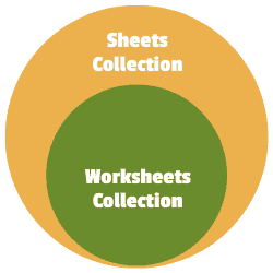
- The ‘Worksheets’ collection would refer to the collection of all the worksheet objects in a workbook. In the above example, the Worksheets collection would consist of three worksheets.
- The ‘Sheets’ collection would refer to all the worksheets as well as chart sheets in the workbook. In the above example, it would have four elements – 3 Worksheets + 1 Chart sheet.
If you have a workbook that only has worksheets and no chart sheets, then ‘Worksheets’ and ‘Sheets’ collection is the same.
But when you have one or more chart sheets, the ‘Sheets’ collection would be bigger than the ‘Worksheets’ collection
Sheets = Worksheets + Chart Sheets
Now with this distinction, I recommend being as specific as possible when writing a VBA code.
So if you have to refer to worksheets only, use the ‘Worksheets’ collection, and if you have to refer to all sheets (including chart sheets), the use the ‘Sheets’ collection.
In this tutorial, I will be using the ‘Worksheets’ collection only.
Referencing a Worksheet in VBA
There are many different ways you can use to refer to a worksheet in VBA.
Understanding how to refer to worksheets would help you write better code, especially when you’re using loops in your VBA code.
Using the Worksheet Name
The easiest way to refer to a worksheet is to use its name.
For example, suppose you have a workbook with three worksheets – Sheet 1, Sheet 2, Sheet 3.
And you want to activate Sheet 2.
You can do that using the following code:

Sub ActivateSheet()
Worksheets("Sheet2").Activate
End Sub
The above code asks VBA to refer to Sheet2 in the Worksheets collection and activate it.
Since we are using the exact sheet name, you can also use the Sheets collection here. So the below code would also do that same thing.
Sub ActivateSheet()
Sheets("Sheet2").Activate
End Sub
Using the Index Number
While using the sheet name is an easy way to refer to a worksheet, sometimes, you may not know the exact name of the worksheet.
For example, if you’re using a VBA code to add a new worksheet to the workbook, and you don’t know how many worksheets are already there, you would not know the name of the new worksheet.
In this case, you can use the index number of the worksheets.
Suppose you have the following sheets in a workbook:
The below code would activate Sheet2:
Sub ActivateSheet()
Worksheets(2).Activate
End Sub
Note that we have used index number 2 in Worksheets(2). This would refer to the second object in the collection of the worksheets.
Now, what happens when you use 3 as the index number?
It will select Sheet3.
If you’re wondering why it selected Sheet3, as it’s clearly the fourth object.
This happens because a chart sheet is not a part of the worksheets collection.
So when we use the index numbers in the Worksheets collection, it will only refer to the worksheets in the workbook (and ignore the chart sheets).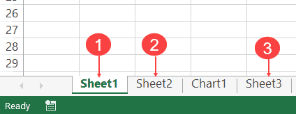
On the contrary, if you’re using Sheets, Sheets(1) would refer to Sheets1, Sheets(2) would refer to Sheet2, Sheets(3) would refer to Chart1 and Sheets(4) would refer to Sheet3.
This technique of using index number is useful when you want to loop through all the worksheets in a workbook. You can count the number of worksheets and then loop through these using this count (we will see how to do this later in this tutorial).
Note: The index number goes from left to right. So if you shift Sheet2 to the left of Sheet1, then Worksheets(1) would refer to Sheet2.
Using the Worksheet Code Name
One of the drawbacks of using the sheet name (as we saw in the section above) is that a user can change it.
And if the sheet name has been changed, your code wouldn’t work until you change the name of the worksheet in the VBA code as well.
To tackle this problem, you can use the code name of the worksheet (instead of the regular name that we have been using so far). A code name can be assigned in the VB Editor and doesn’t change when you change the name of the sheet from the worksheet area.
To give your worksheet a code name, follow the below steps:
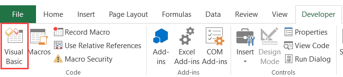
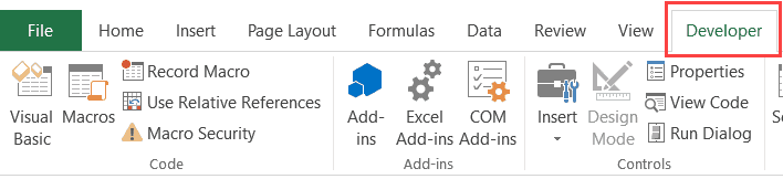
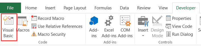
- Click the Developer tab.
- Click the Visual Basic button. This will open the VB Editor.

- Click the View option in the menu and click on Project Window. This will make the Properties pane visible. If the Properties pane is already visible, skip this step.
- Click on the sheet name in the project explorer that you want to rename.
- In the Properties pane, change the name in the field in front of (Name). Note that you can’t have spaces in the name.

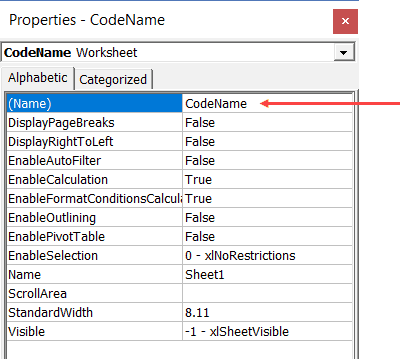
The above steps would change the name of your Worksheet in the VBA backend. In the Excel worksheet view, you can name the worksheet whatever you want, but in the backend, it will respond to both the names – the sheet name and the code name.
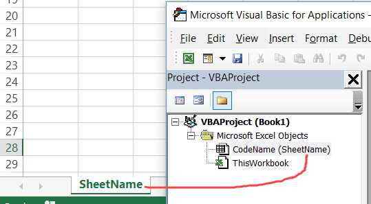
In the above image, the sheet name is ‘SheetName’ and the code name is ‘CodeName’. Even if you change the sheet name on the worksheet, the code name still remains the same.
Now, you can use either the Worksheets collection to refer to the worksheet or use the codename.
For example, both the line will activate the worksheet.
Worksheets("Sheetname").Activate
CodeName.Activate
The difference in these two is that if you change the name of the worksheet, the first one wouldn’t work. But the second line would continue to work even with the changed name. The second line (using the CodeName) is also shorter and easier to use.
Referring to a Worksheet in a Different Workbook
If you want to refer to a worksheet in a different workbook, that workbook needs to be open while the code runs, and you need to specify the name of the workbook and the worksheet that you want to refer to.
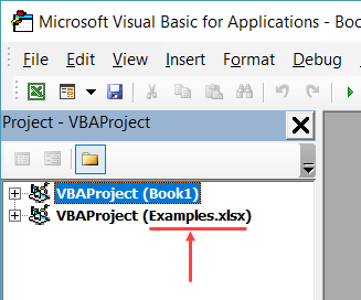
For example, if you have a workbook with the name Examples and you want to activate Sheet1 in the Example workbook, you need to use the below code:
Sub SheetActivate()
Workbooks("Examples.xlsx").Worksheets("Sheet1").Activate
End Sub
Note that if the workbook has been saved, you need to use the file name along with the extension. If you’re not sure what name to use, take help from Project Explorer.
In case the workbook has not been saved, you don’t need to use the file extension.
Adding a Worksheet
The below code would add a worksheet (as the first worksheet – i.e., as the leftmost sheet in the sheet tab).
Sub AddSheet()
Worksheets.Add
End Sub
It takes the default name Sheet2 (or any other number based on how many sheets are already there).
If you want a worksheet to be added before a specific worksheet (say Sheet2), then you can use the below code.
Sub AddSheet()
Worksheets.Add Before:=Worksheets("Sheet2")
End Sub
The above code tells VBA to add a sheet and then uses the ‘Before’ statement to specify the worksheet before which the new worksheet should to be inserted.
Similarly, you can also add a sheet after a worksheet (say Sheet2), using the below code:
Sub AddSheet()
Worksheets.Add After:=Worksheets("Sheet2")
End Sub
If you want the new sheet to be added to the end of the sheets, you need to first know how many sheets are there. The following code first counts the number of sheets, and the adds the new sheet after the last sheet (to which we refer using the index number).
Sub AddSheet()
Dim SheetCount As Integer
SheetCount = Worksheets.Count
Worksheets.Add After:=Worksheets(SheetCount)
End Sub
Deleting a Worksheet
The below code would delete the active sheet from the workbook.
Sub DeleteSheet()
ActiveSheet.Delete
End Sub
The above code would show a warning prompt before deleting the worksheet.
If you don’t want to see the warning prompt, use the below code:
Sub DeleteSheet()
Application.DisplayAlerts = False
ActiveSheet.Delete
Application.DisplayAlerts = True
End Sub
When Application.DisplayAlerts is set to False, it will not show you the warning prompt. If you use it, remember to set it back to True at the end of the code.
Remember that you can’t undo this delete, so use the above code when you’re absolutely sure.
If you want to delete a specific sheet, you can do that using the following code:
Sub DeleteSheet()
Worksheets("Sheet2").Delete
End Sub
You can also use the code name of the sheet to delete it.
Sub DeleteSheet()
Sheet5.Delete
End Sub
Renaming the Worksheets
You can modify the name property of the Worksheet to change its name.
The following code will change the name of Sheet1 to ‘Summary’.
Sub RenameSheet()
Worksheets("Sheet1").Name = "Summary"
End Sub
You can combine this with the adding sheet method to have a set of sheets with specific names.
For example, if you want to insert four sheets with the name 2018 Q1, 2018 Q2, 2018 Q3, and 2018 Q4, you can use the below code.
Sub RenameSheet()
Dim Countsheets As Integer
Countsheets = Worksheets.Count
For i = 1 To 4
Worksheets.Add after:=Worksheets(Countsheets + i - 1)
Worksheets(Countsheets + i).Name = "2018 Q" & i
Next i
End Sub
In the above code, we first count the number of sheets and then use a For Next loop to insert new sheets at the end. As the sheet is added, the code also renames it.
Assigning Worksheet Object to a Variable
When working with worksheets, you can assign a worksheet to an object variable, and then use the variable instead of the worksheet references.
For example, if you want to add a year prefix to all the worksheets, instead of counting the sheets and the running the loop that many numbers of times, you can use the object variable.
Here is the code that will add 2018 as a prefix to all the worksheet’s names.
Sub RenameSheet()
Dim Ws As Worksheet
For Each Ws In Worksheets
Ws.Name = "2018 - " & Ws.Name
Next Ws
End Sub
The above code declares a variable Ws as the worksheet type (using the line ‘Dim Ws As Worksheet’).
Now, we don’t need to count the number of sheets to loop through these. Instead, we can use ‘For each Ws in Worksheets’ loop. This will allow us to go through all the sheets in the worksheets collection. It doesn’t matter whether there are 2 sheets or 20 sheets.
While the above code allows us to loop through all the sheets, you can also assign a specific sheet to a variable.
In the below code, we assign the variable Ws to Sheet2 and use it to access all of Sheet2’s properties.
Sub RenameSheet()
Dim Ws As Worksheet
Set Ws = Worksheets("Sheet2")
Ws.Name = "Summary"
Ws.Protect
End Sub
Once you set a worksheet reference to an object variable (using the SET statement), that object can be used instead of the worksheet reference. This can be helpful when you have a long complicated code and you want to change the reference. Instead of making the change everywhere, you can simply make the change in the SET statement.
Note that the code declares the Ws object as the Worksheet type variable (using the line Dim Ws as Worksheet).
Hide Worksheets Using VBA (Hidden + Very Hidden)
Hiding and Unhiding worksheets in Excel is a straightforward task.
You can hide a worksheet and the user would not see it when he/she opens the workbook. However, they can easily unhide the worksheet by right-clicking on any sheet tab.
But what if you don’t want them to be able to unhide the worksheet(s).
You can do this using VBA.
The code below would hide all the worksheets in the workbook (except the active sheet), such that you can not unhide it by right-clicking on the sheet name.
Sub HideAllExcetActiveSheet()
Dim Ws As Worksheet
For Each Ws In ThisWorkbook.Worksheets
If Ws.Name <> ActiveSheet.Name Then Ws.Visible = xlSheetVeryHidden
Next Ws
End Sub
In the above code, the Ws.Visible property is changed to xlSheetVeryHidden.
- When the Visible property is set to xlSheetVisible, the sheet is visible in the worksheet area (as worksheet tabs).
- When the Visible property is set to xlSheetHidden, the sheet is hidden but the user can unhide it by right-clicking on any sheet tab.
- When the Visible property is set to xlSheetVeryHidden, the sheet is hidden and cannot be unhidden from worksheet area. You need to use a VBA code or the properties window to unhide it.
If you want to simply hide sheets, that can be unhidden easily, use the below code:
Sub HideAllExceptActiveSheet()
Dim Ws As Worksheet
For Each Ws In ThisWorkbook.Worksheets
If Ws.Name <> ActiveSheet.Name Then Ws.Visible = xlSheetHidden
Next Ws
End Sub
The below code would unhide all the worksheets (both hidden and very hidden).
Sub UnhideAllWoksheets()
Dim Ws As Worksheet
For Each Ws In ThisWorkbook.Worksheets
Ws.Visible = xlSheetVisible
Next Ws
End Sub
Related Article: Unhide All Sheets In Excel (at one go)
Hide Sheets Based on the Text in it
Suppose you have multiple sheets with the name of different departments or years and you want to hide all the sheets except the ones that have the year 2018 in it.
You can do this using a VBA INSTR function.
The below code would hide all the sheets except the ones with the text 2018 in it.
Sub HideWithMatchingText()
Dim Ws As Worksheet
For Each Ws In Worksheets
If InStr(1, Ws.Name, "2018", vbBinaryCompare) = 0 Then
Ws.Visible = xlSheetHidden
End If
Next Ws
End Sub
In the above code, the INSTR function returns the position of the character where it finds the matching string. If it doesn’t find the matching string, it returns 0.
The above code checks whether the name has the text 2018 in it. If it does, nothing happens, else the worksheet is hidden.
You can take this a step further by having the text in a cell and using that cell in the code. This will allow you to have a value in the cell and then when you run the macro, all the sheets, except the one with the matching text in it, would remain visible (along with the sheets where you’re entering the value in the cell).
Sorting the Worksheets in an Alphabetical Order
Using VBA, you can quickly sort the worksheets based on their names.
For example, if you have a workbook that has sheets for different department or years, then you can use the below code to quickly sort these sheets in an ascending order.
Sub SortSheetsTabName()
Application.ScreenUpdating = False
Dim ShCount As Integer, i As Integer, j As Integer
ShCount = Sheets.Count
For i = 1 To ShCount - 1
For j = i + 1 To ShCount
If Sheets(j).Name < Sheets(i).Name Then
Sheets(j).Move before:=Sheets(i)
End If
Next j
Next i
Application.ScreenUpdating = True
End Sub
Note that this code works well with text names and in most of the cases with years and numbers too. But it can give you the wrong results in case you have the sheet names as 1,2,11. It will sort and give you the sequence 1, 11, 2. This is because it does the comparison as text and considers 2 bigger than 11.
Protect/Unprotect All the Sheets at One Go
If you have a lot of worksheets in a workbook and you want to protect all the sheets, you can use the VBA code below.
It allows you to specify the password within the code. You will need this password to unprotect the worksheet.
Sub ProtectAllSheets()
Dim ws As Worksheet
Dim password As String
password = "Test123" 'replace Test123 with the password you want
For Each ws In Worksheets
ws.Protect password:=password
Next ws
End Sub
The following code would unprotect all the sheets in one go.
Sub ProtectAllSheets()
Dim ws As Worksheet
Dim password As String
password = "Test123" 'replace Test123 with the password you used while protecting
For Each ws In Worksheets
ws.Unprotect password:=password
Next ws
End Sub
Creating a Table of Contents of All Worksheets (with Hyperlinks)
If you have a set of worksheets in the workbook and you want to quickly insert a summary sheet which has the links to all the sheets, you can use the below code.
Sub AddIndexSheet()
Worksheets.Add
ActiveSheet.Name = "Index"
For i = 2 To Worksheets.Count
ActiveSheet.Hyperlinks.Add Anchor:=Cells(i - 1, 1), _
Address:="", SubAddress:=Worksheets(i).Name & "!A1", _
TextToDisplay:=Worksheets(i).Name
Next i
End Sub
The above code inserts a new worksheet and names it Index.
It then loops through all the worksheets and creates a hyperlink for all the worksheets in the Index sheet.
Where to Put the VBA Code
Wondering where the VBA code goes in your Excel workbook?
Excel has a VBA backend called the VBA editor. You need to copy and paste the code into the VB Editor module code window.
Here are the steps to do this:
- Go to the Developer tab.

- Click on the Visual Basic option. This will open the VB editor in the backend.
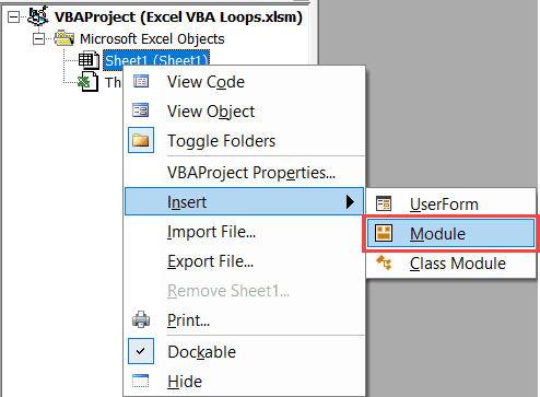
- In the Project Explorer pane in the VB Editor, right-click on any object for the workbook in which you want to insert the code. If you don’t see the Project Explorer go to the View tab and click on Project Explorer.
- Go to Insert and click on Module. This will insert a module object for your workbook.

- Copy and paste the code in the module window.
You May Also Like the Following Excel VBA Tutorials:
- Working with Workbooks using VBA.
- Using IF Then Else Statements in VBA.
- For Next Loop in VBA.
- Creating a User-Defined Function in Excel.
- How to Record a Macro in Excel.
- How to Run a Macro in Excel.
- Excel VBA Events – An Easy (and Complete) Guide.
- How to Create an Add-in in Excel.
- How to Save and Reuse Macro using Excel Personal Macro Workbook.
- Using Active Cell in VBA in Excel (Examples)
- How to Open Excel Files Using VBA (Examples)