
Excel for Microsoft 365 Excel for Microsoft 365 for Mac Excel 2021 for Mac Excel 2019 Excel 2019 for Mac Excel 2016 Excel 2016 for Mac Excel 2013 Excel 2010 More…Less
If you have tasks in Microsoft Excel that you do repeatedly, you can record a macro to automate those tasks. A macro is an action or a set of actions that you can run as many times as you want. When you create a macro, you are recording your mouse clicks and keystrokes. After you create a macro, you can edit it to make minor changes to the way it works.
Suppose that every month, you create a report for your accounting manager. You want to format the names of the customers with overdue accounts in red, and also apply bold formatting. You can create and then run a macro that quickly applies these formatting changes to the cells you select.
How?
|
|
Before you record a macro Macros and VBA tools can be found on the Developer tab, which is hidden by default, so the first step is to enable it. For more information, see Show the Developer tab. |


|
|
Record a macro
|

|
|
Take a closer look at the macro You can learn a little about the Visual Basic programming language by editing a macro. To edit a macro, in the Code group on the Developer tab, click Macros, select the name of the macro, and click Edit. This starts the Visual Basic Editor. See how the actions that you recorded appear as code. Some of the code will probably be clear to you, and some of it may be a little mysterious. Experiment with the code, close the Visual Basic Editor, and run your macro again. This time, see if anything different happens! |

Next steps
-
To learn more about creating macros, see Create or delete a macro.
-
To learn about how to run a macro, see Run a macro.
How?
|
|
Before you record a macro Make sure the Developer tab is visible on the ribbon. By default, the Developer tab is not visible, so do the following:
|
|
|
Record a macro
|
|
|
Take a closer look at the macro You can learn a little about the Visual Basic programming language by editing a macro. To edit a macro, in the Developer tab, click Macros, select the name of the macro, and click Edit. This starts the Visual Basic Editor. See how the actions that you recorded appear as code. Some of the code will probably be clear to you, and some of it may be a little mysterious. Experiment with the code, close the Visual Basic Editor, and run your macro again. This time, see if anything different happens! |
Need more help?
You can always ask an expert in the Excel Tech Community or get support in the Answers community.
Need more help?
#Руководства
- 23 май 2022
-

0
Как с помощью макросов автоматизировать рутинные задачи в Excel? Какие команды они выполняют? Как создать макрос новичку? Разбираемся на примере.
Иллюстрация: Meery Mary для Skillbox Media

Рассказывает просто о сложных вещах из мира бизнеса и управления. До редактуры — пять лет в банке и три — в оценке имущества. Разбирается в Excel, финансах и корпоративной жизни.
Макрос (или макрокоманда) в Excel — алгоритм действий в программе, который объединён в одну команду. С помощью макроса можно выполнить несколько шагов в Excel, нажав на одну кнопку в меню или на сочетание клавиш.
Обычно макросы используют для автоматизации рутинной работы — вместо того чтобы выполнять десяток повторяющихся действий, пользователь записывает одну команду и затем запускает её, когда нужно совершить эти действия снова.
Например, если нужно добавить название компании в несколько десятков документов и отформатировать его вид под корпоративный дизайн, можно делать это в каждом документе отдельно, а можно записать ход действий при создании первого документа в макрос — и затем применить его ко всем остальным. Второй вариант будет гораздо проще и быстрее.
В статье разберёмся:
- как работают макросы и как с их помощью избавиться от рутины в Excel;
- какие способы создания макросов существуют и как подготовиться к их записи;
- как записать и запустить макрос начинающим пользователям — на примере со скриншотами.
Общий принцип работы макросов такой:
- Пользователь записывает последовательность действий, которые нужно выполнить в Excel, — о том, как это сделать, поговорим ниже.
- Excel обрабатывает эти действия и создаёт для них одну общую команду. Получается макрос.
- Пользователь запускает этот макрос, когда ему нужно выполнить эту же последовательность действий ещё раз. При записи макроса можно задать комбинацию клавиш или создать новую кнопку на главной панели Excel — если нажать на них, макрос запустится автоматически.
Макросы могут выполнять любые действия, которые в них запишет пользователь. Вот некоторые команды, которые они умеют делать в Excel:
- Автоматизировать повторяющиеся процедуры.
Например, если пользователю нужно каждый месяц собирать отчёты из нескольких файлов в один, а порядок действий каждый раз один и тот же, можно записать макрос и запускать его ежемесячно.
- Объединять работу нескольких программ Microsoft Office.
Например, с помощью одного макроса можно создать таблицу в Excel, вставить и сохранить её в документе Word и затем отправить в письме по Outlook.
- Искать ячейки с данными и переносить их в другие файлы.
Этот макрос пригодится, когда нужно найти информацию в нескольких объёмных документах. Макрос самостоятельно отыщет её и принесёт в заданный файл за несколько секунд.
- Форматировать таблицы и заполнять их текстом.
Например, если нужно привести несколько таблиц к одному виду и дополнить их новыми данными, можно записать макрос при форматировании первой таблицы и потом применить его ко всем остальным.
- Создавать шаблоны для ввода данных.
Команда подойдёт, когда, например, нужно создать анкету для сбора данных от сотрудников. С помощью макроса можно сформировать такой шаблон и разослать его по корпоративной почте.
- Создавать новые функции Excel.
Если пользователю понадобятся дополнительные функции, которых ещё нет в Excel, он сможет записать их самостоятельно. Все базовые функции Excel — это тоже макросы.
Все перечисленные команды, а также любые другие команды пользователя можно комбинировать друг с другом и на их основе создавать макросы под свои потребности.
В Excel и других программах Microsoft Office макросы создаются в виде кода на языке программирования VBA (Visual Basic for Applications). Этот язык разработан в Microsoft специально для программ компании — он представляет собой упрощённую версию языка Visual Basic. Но это не значит, что для записи макроса нужно уметь кодить.
Есть два способа создания макроса в Excel:
- Написать макрос вручную.
Это способ для продвинутых пользователей. Предполагается, что они откроют окно Visual Basic в Еxcel и самостоятельно напишут последовательность действий для макроса в виде кода.
- Записать макрос с помощью кнопки меню Excel.
Способ подойдёт новичкам. В этом варианте Excel запишет программный код вместо пользователя. Нужно нажать кнопку записи и выполнить все действия, которые планируется включить в макрос, и после этого остановить запись — Excel переведёт каждое действие и выдаст алгоритм на языке VBA.
Разберёмся на примере, как создать макрос с помощью второго способа.
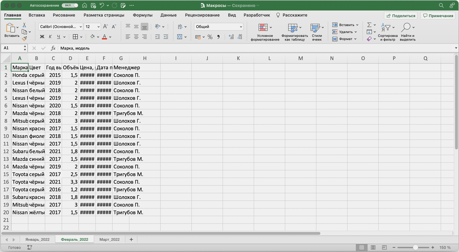
Допустим, специальный сервис автосалона выгрузил отчёт по продажам за три месяца первого квартала в формате таблиц Excel. Эти таблицы содержат всю необходимую информацию, но при этом никак не отформатированы: колонки слиплись друг с другом и не видны полностью, шапка таблицы не выделена и сливается с другими строками, часть данных не отображается.
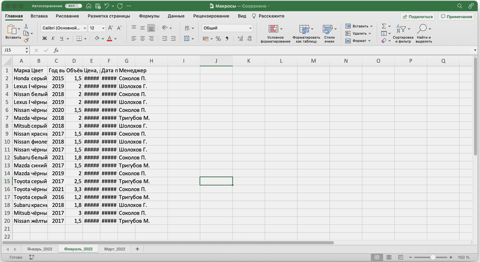
Скриншот: Skillbox Media
Пользоваться таким отчётом неудобно — нужно сделать его наглядным. Запишем макрос при форматировании таблицы с продажами за январь и затем применим его к двум другим таблицам.
Готовимся к записи макроса
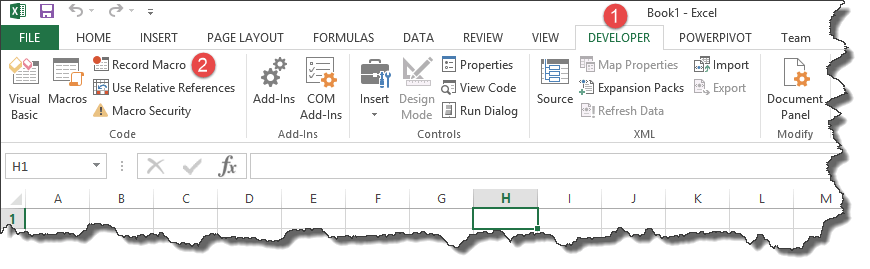
Кнопки для работы с макросами в Excel находятся во вкладке «Разработчик». Эта вкладка по умолчанию скрыта, поэтому для начала разблокируем её.
В операционной системе Windows это делается так: переходим во вкладку «Файл» и выбираем пункты «Параметры» → «Настройка ленты». В открывшемся окне в разделе «Основные вкладки» находим пункт «Разработчик», отмечаем его галочкой и нажимаем кнопку «ОК» → в основном меню Excel появляется новая вкладка «Разработчик».
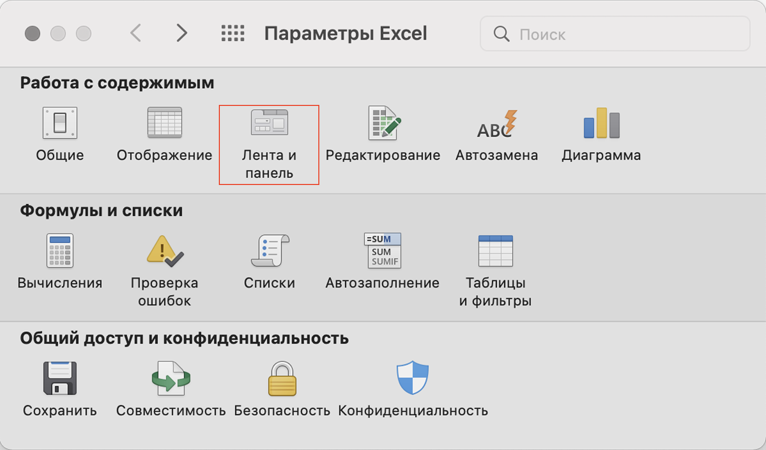
В операционной системе macOS это нужно делать по-другому. В самом верхнем меню нажимаем на вкладку «Excel» и выбираем пункт «Параметры…».
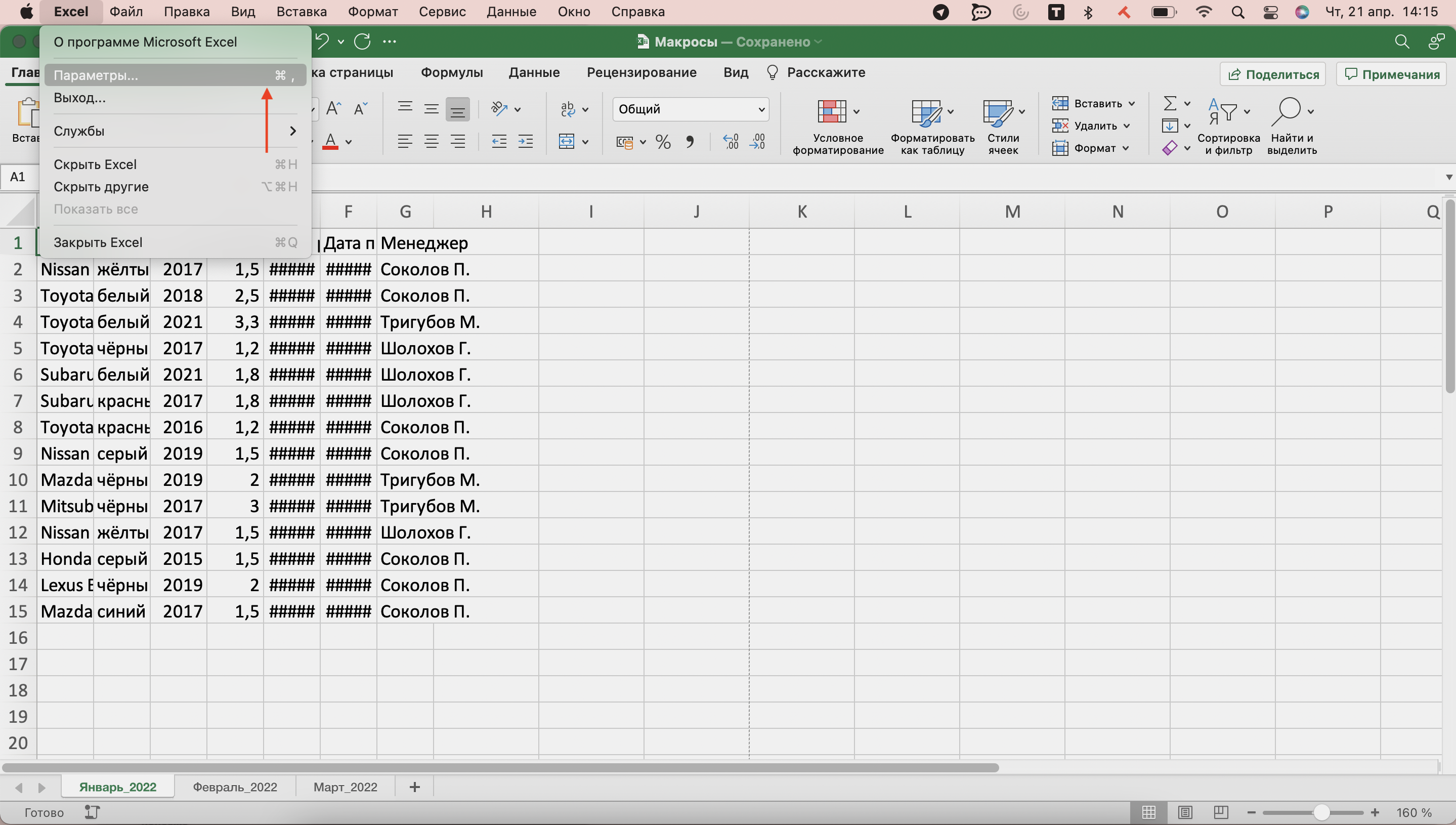
Скриншот: Skillbox Media
В появившемся окне нажимаем кнопку «Лента и панель».
Скриншот: Skillbox Media
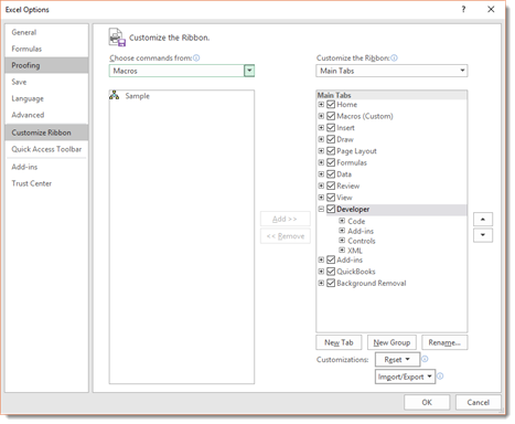
Затем в правой панели «Настроить ленту» ищем пункт «Разработчик» и отмечаем его галочкой. Нажимаем «Сохранить».
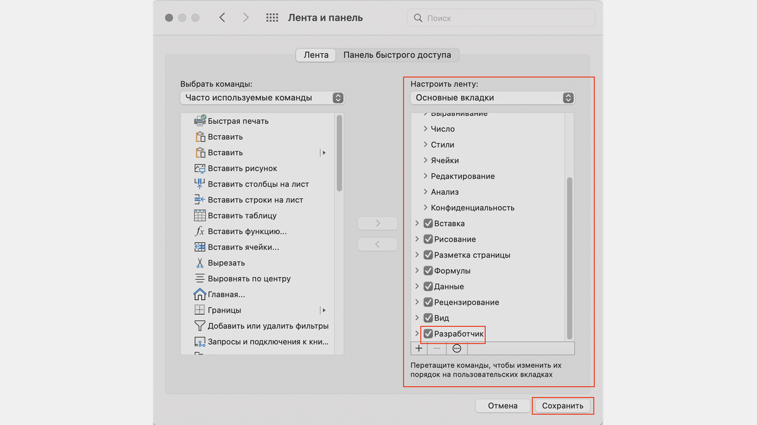
Скриншот: Skillbox Media
Готово — вкладка «Разработчик» появилась на основной панели Excel.
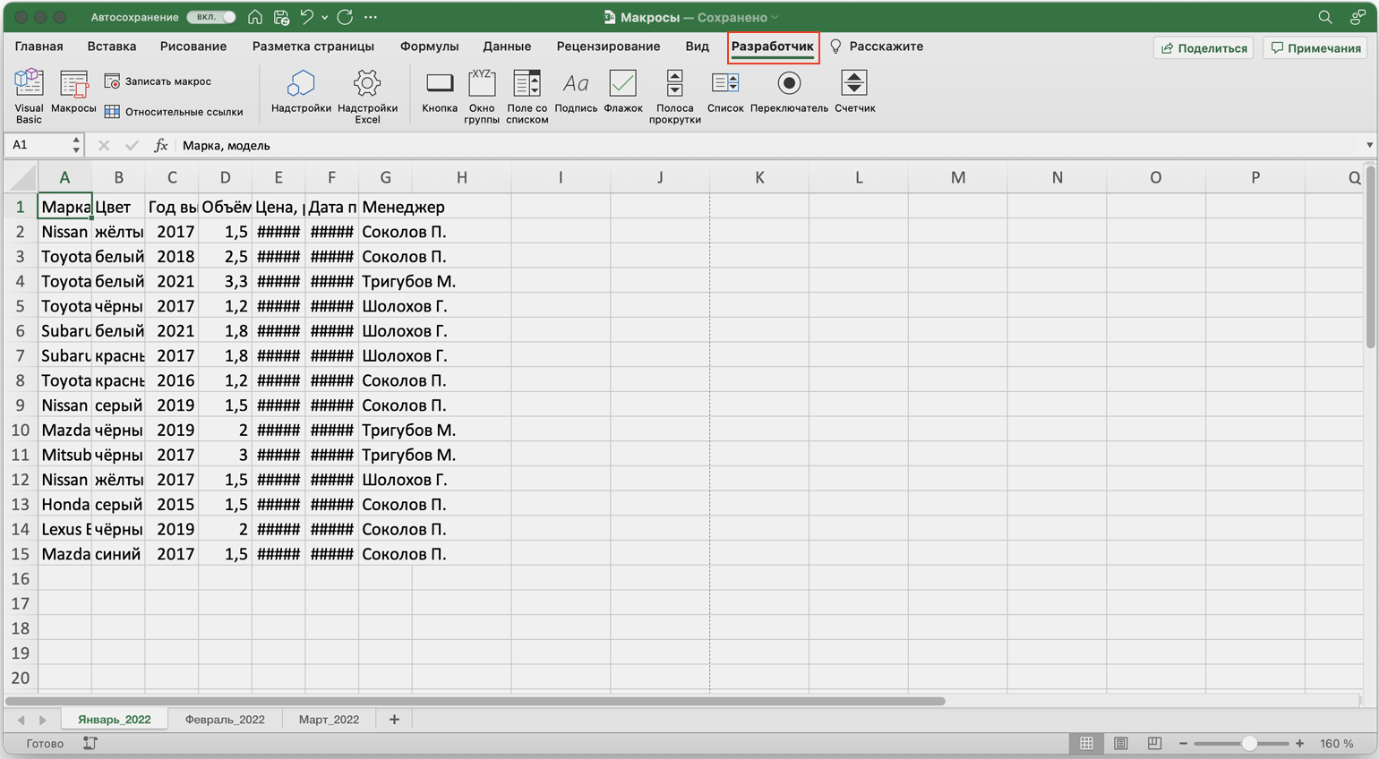
Скриншот: Skillbox Media
Чтобы Excel смог сохранить и в дальнейшем использовать макрос, нужно пересохранить документ в формате, который поддерживает макросы. Это делается через команду «Сохранить как» на главной панели. В появившемся меню нужно выбрать формат «Книга Excel с поддержкой макросов».
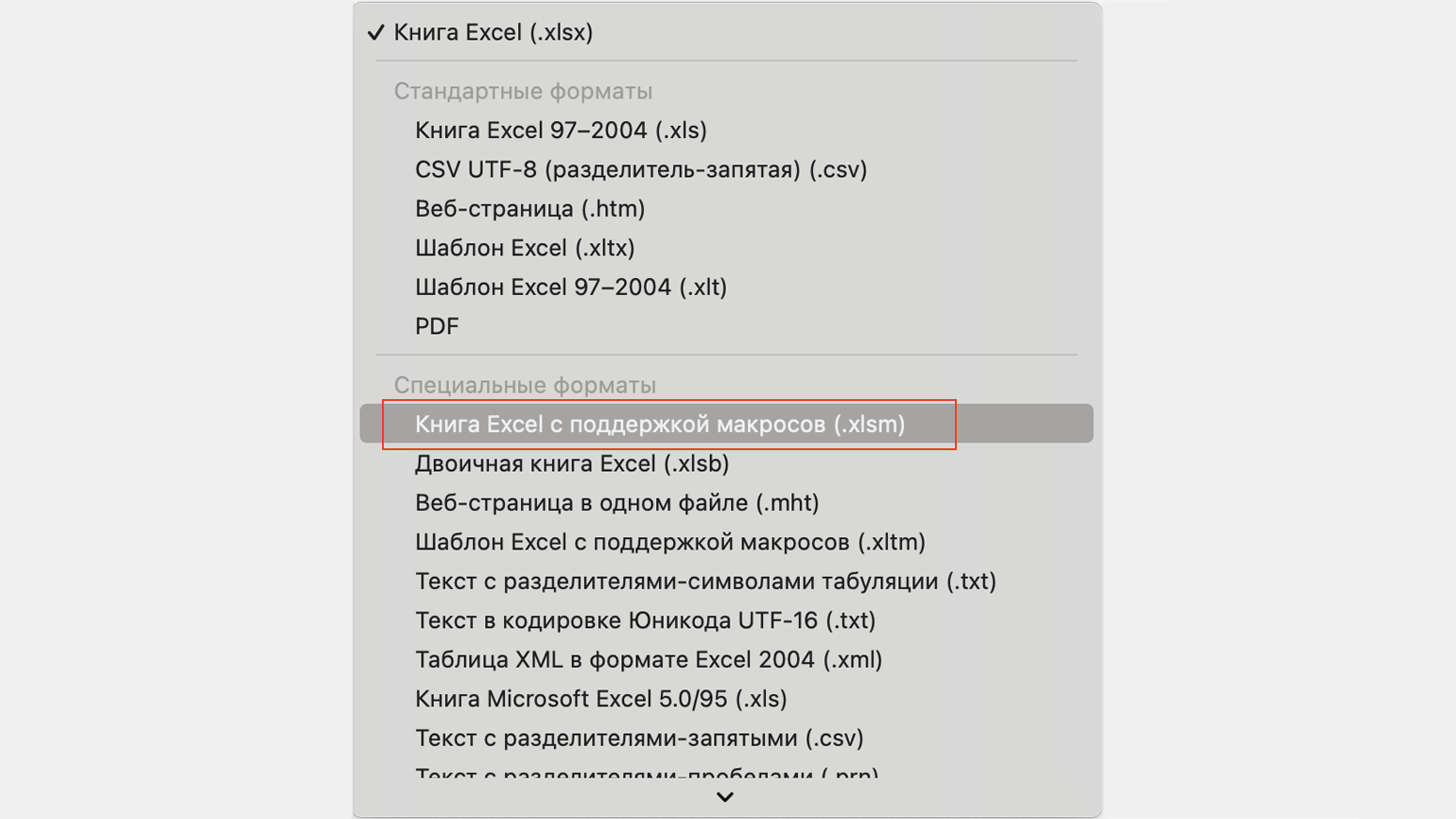
Скриншот: Skillbox Media
Перед началом записи макроса важно знать об особенностях его работы:
- Макрос записывает все действия пользователя.
После старта записи макрос начнёт регистрировать все клики мышки и все нажатия клавиш. Поэтому перед записью последовательности лучше хорошо отработать её, чтобы не добавлять лишних действий и не удлинять код. Если требуется записать длинную последовательность задач — лучше разбить её на несколько коротких и записать несколько макросов.
- Работу макроса нельзя отменить.
Все действия, которые выполняет запущенный макрос, остаются в файле навсегда. Поэтому перед тем, как запускать макрос в первый раз, лучше создать копию всего файла. Если что-то пойдёт не так, можно будет просто закрыть его и переписать макрос в созданной копии.
- Макрос выполняет свой алгоритм только для записанного диапазона таблиц.
Если при записи макроса пользователь выбирал диапазон таблицы, то и при запуске макроса в другом месте он выполнит свой алгоритм только в рамках этого диапазона. Если добавить новую строку, макрос к ней применяться не будет. Поэтому при записи макроса можно сразу выбирать большее количество строк — как это сделать, показываем ниже.
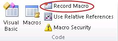
Для начала записи макроса перейдём на вкладку «Разработчик» и нажмём кнопку «Записать макрос».
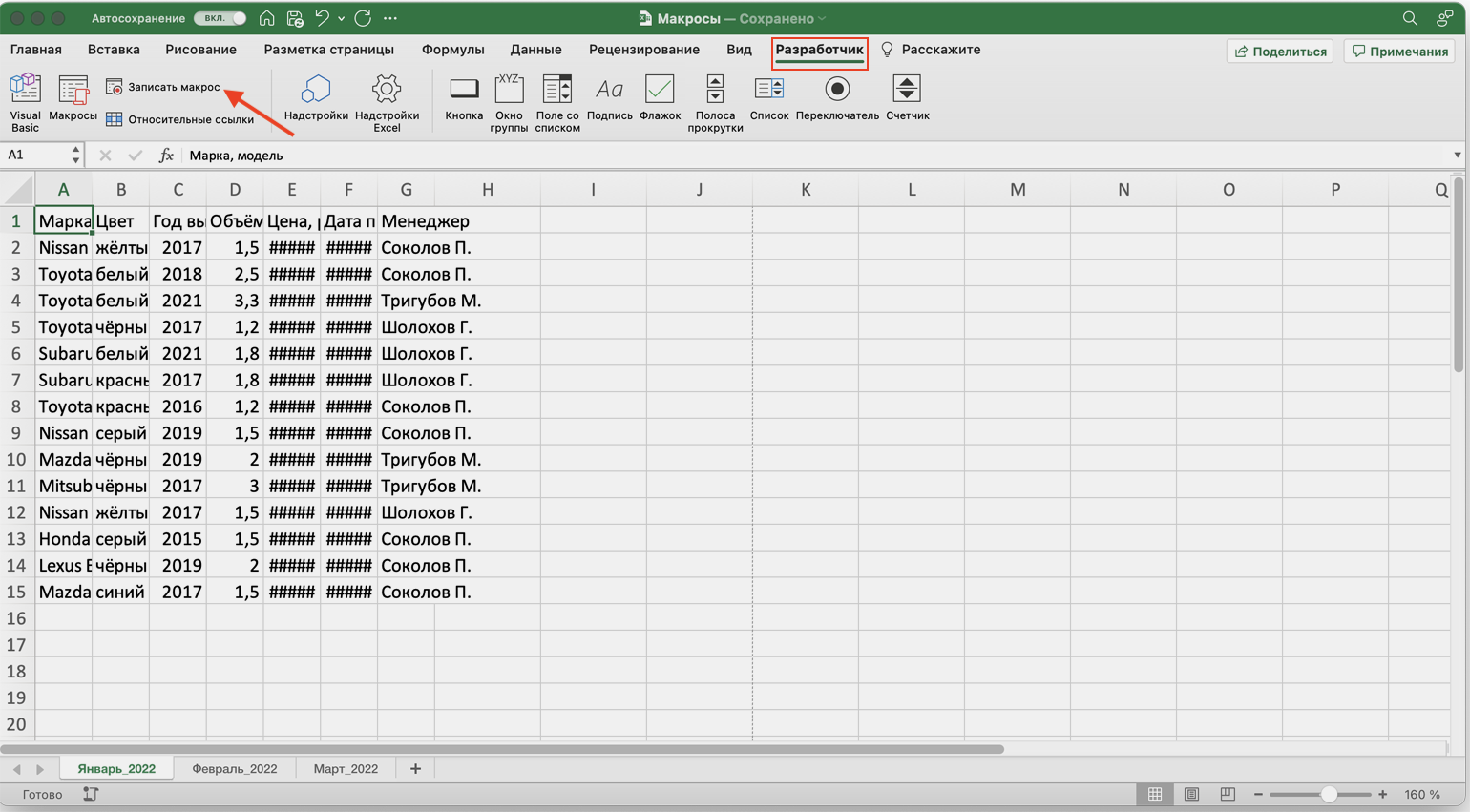
Скриншот: Skillbox Media
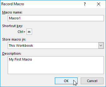
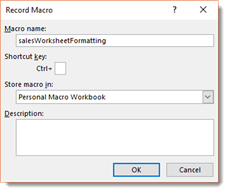
Появляется окно для заполнения параметров макроса. Нужно заполнить поля: «Имя макроса», «Сохранить в», «Сочетание клавиш», «Описание».
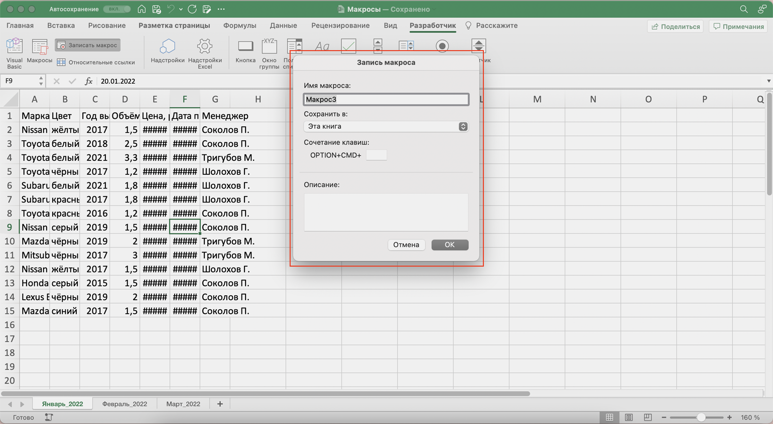
Скриншот: Skillbox Media
«Имя макроса» — здесь нужно придумать и ввести название для макроса. Лучше сделать его логически понятным, чтобы в дальнейшем можно было быстро его найти.
Первым символом в названии обязательно должна быть буква. Другие символы могут быть буквами или цифрами. Важно не использовать пробелы в названии — их можно заменить символом подчёркивания.
«Сохранить в» — здесь нужно выбрать книгу, в которую макрос сохранится после записи.
Если выбрать параметр «Эта книга», макрос будет доступен при работе только в этом файле Excel. Чтобы макрос был доступен всегда, нужно выбрать параметр «Личная книга макросов» — Excel создаст личную книгу макросов и сохранит новый макрос в неё.
«Сочетание клавиш» — здесь к уже выбранным двум клавишам (Ctrl + Shift в системе Windows и Option + Cmd в системе macOS) нужно добавить третью клавишу. Это должна быть строчная или прописная буква, которую ещё не используют в других быстрых командах компьютера или программы Excel.
В дальнейшем при нажатии этих трёх клавиш записанный макрос будет запускаться автоматически.
«Описание» — необязательное поле, но лучше его заполнять. Например, можно ввести туда последовательность действий, которые планируется записать в этом макросе. Так не придётся вспоминать, какие именно команды выполнит этот макрос, если нужно будет запустить его позже. Плюс будет проще ориентироваться среди других макросов.
В нашем случае с форматированием таблицы заполним поля записи макроса следующим образом и нажмём «ОК».
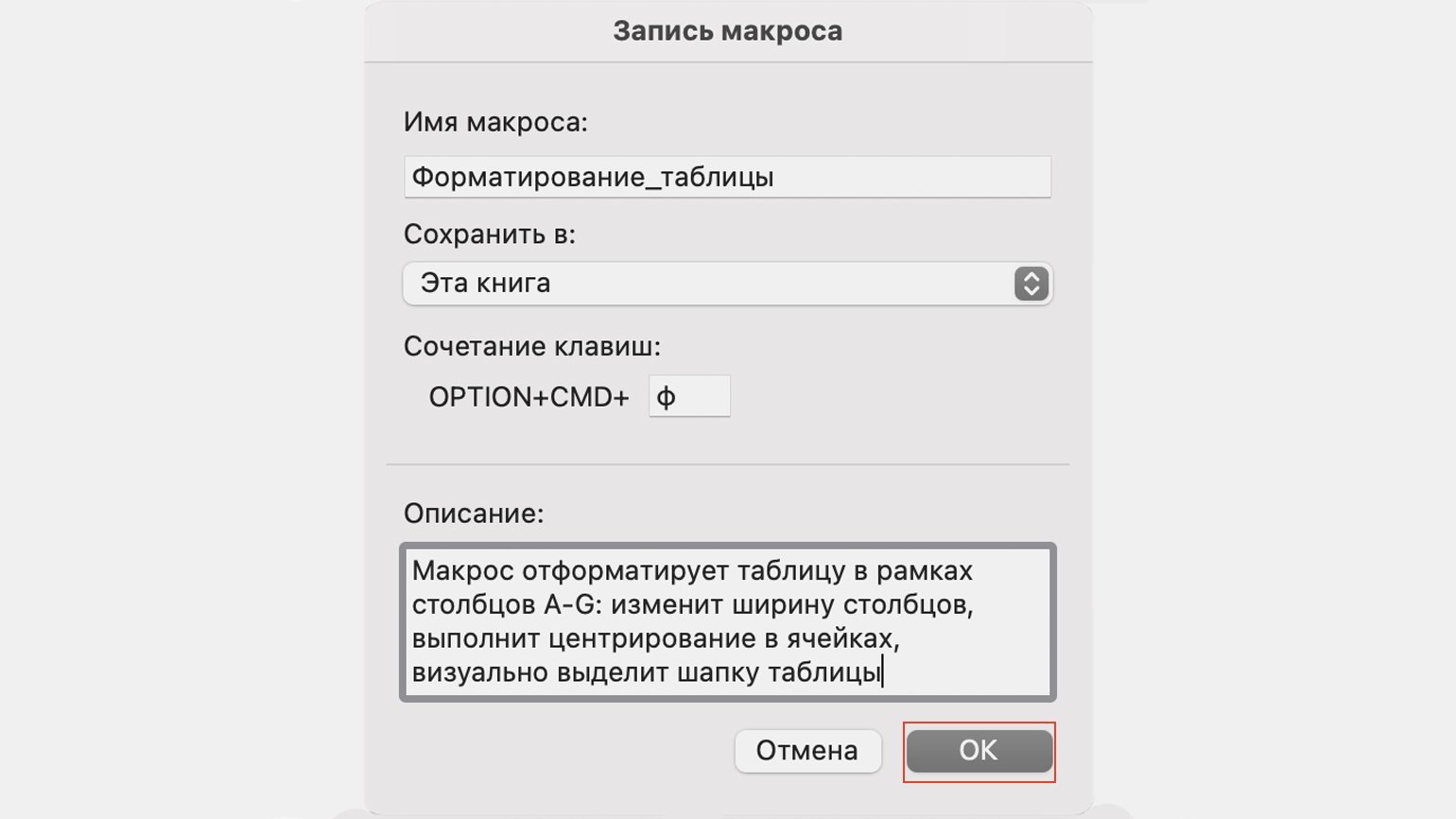
Скриншот: Skillbox Media
После этого начнётся запись макроса — в нижнем левом углу окна Excel появится значок записи.
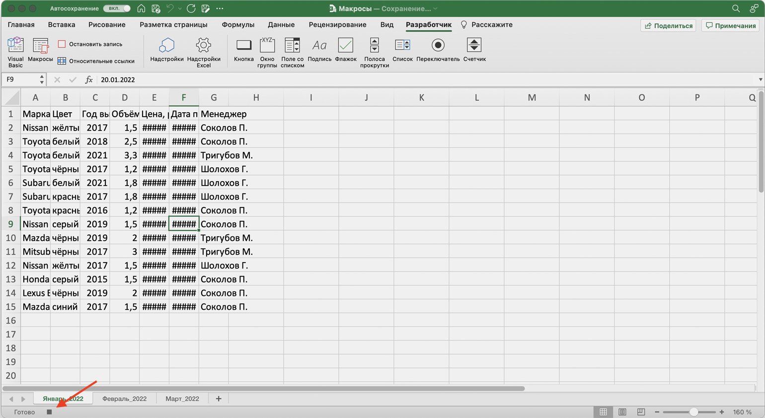
Скриншот: Skillbox Media
Пока идёт запись, форматируем таблицу с продажами за январь: меняем ширину всех столбцов, данные во всех ячейках располагаем по центру, выделяем шапку таблицы цветом и жирным шрифтом, рисуем границы.
Важно: в нашем случае у таблиц продаж за январь, февраль и март одинаковое количество столбцов, но разное количество строк. Чтобы в случае со второй и третьей таблицей макрос сработал корректно, при форматировании выделим диапазон так, чтобы в него попали не только строки самой таблицы, но и строки ниже неё. Для этого нужно выделить столбцы в строке с их буквенным обозначением A–G, как на рисунке ниже.
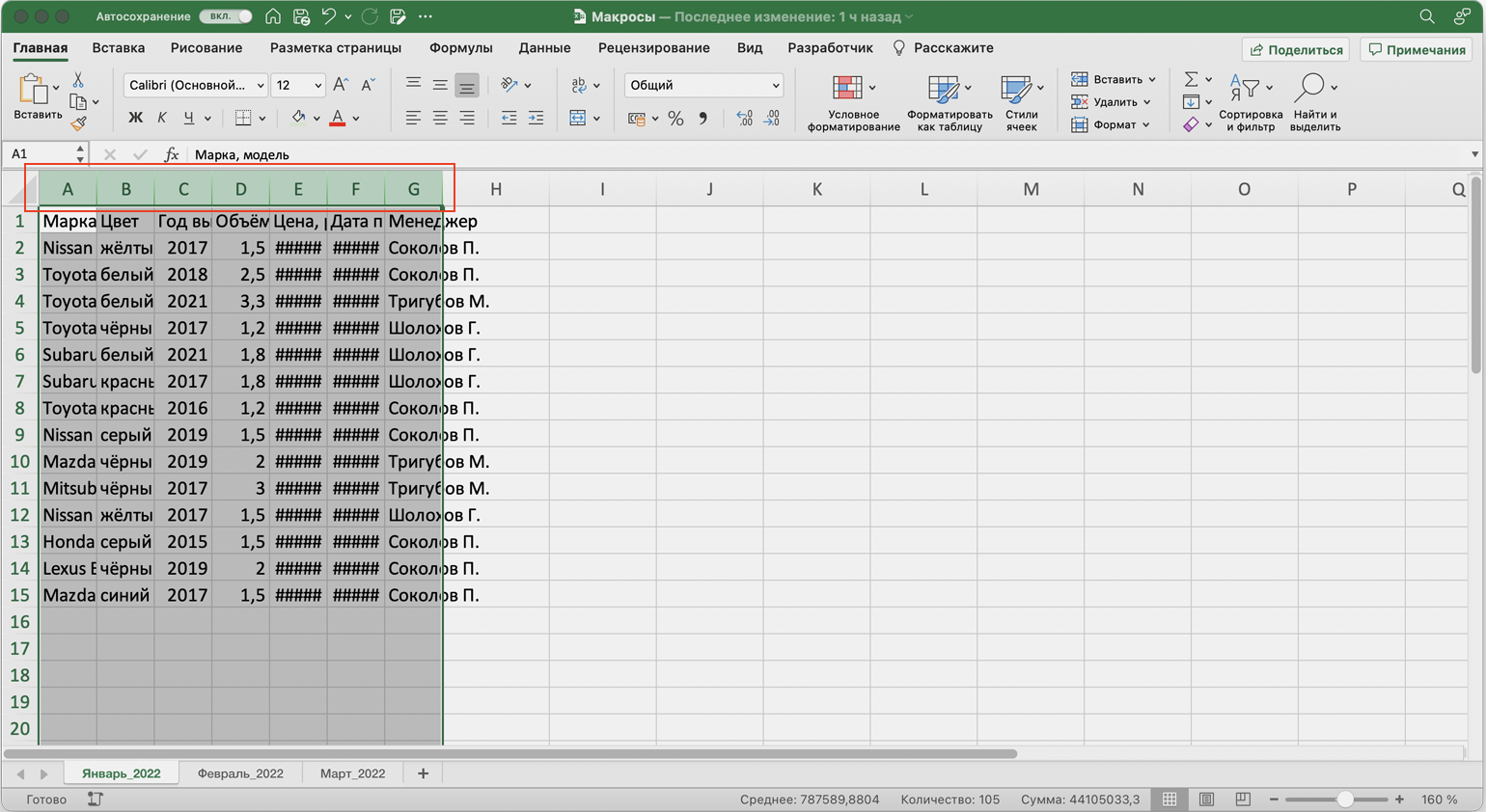
Скриншот: Skillbox Media
Если выбрать диапазон только в рамках первой таблицы, то после запуска макроса в таблице с большим количеством строк она отформатируется только частично.
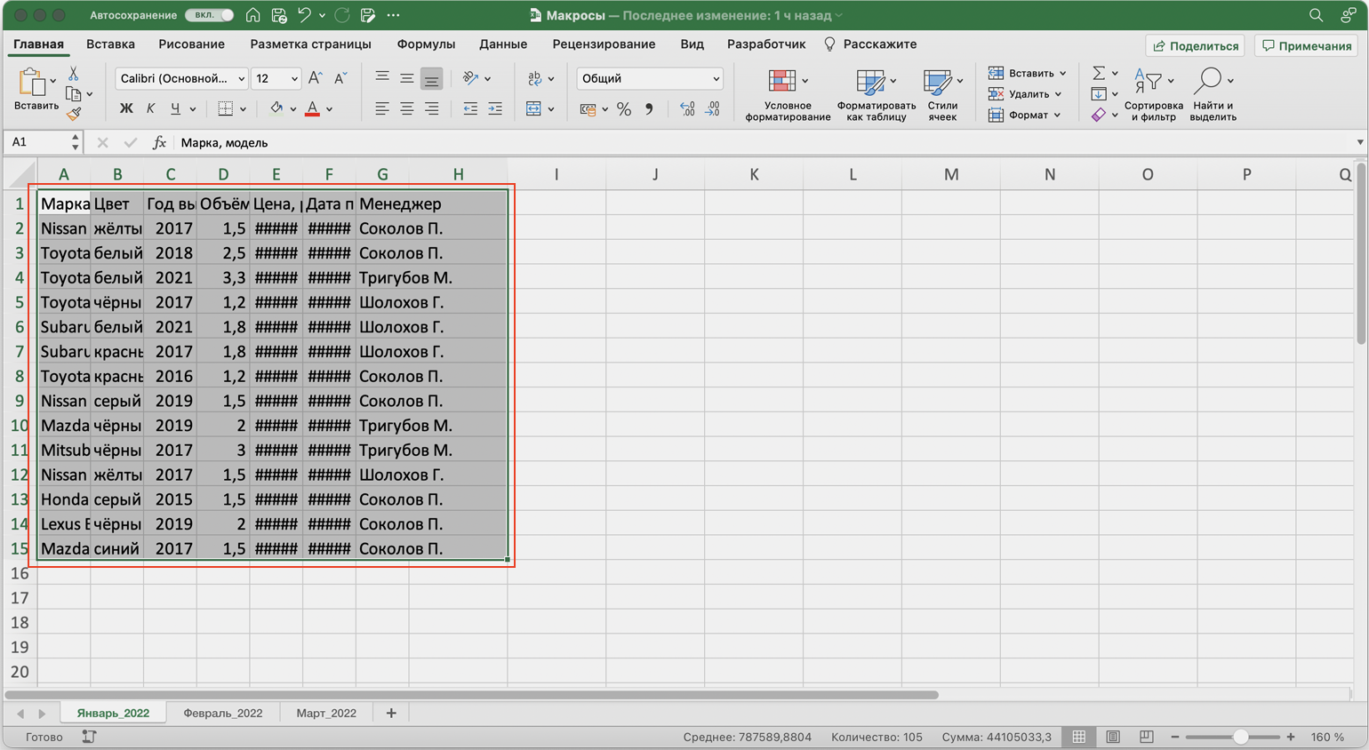
Скриншот: Skillbox Media
После всех манипуляций с оформлением таблица примет такой вид:
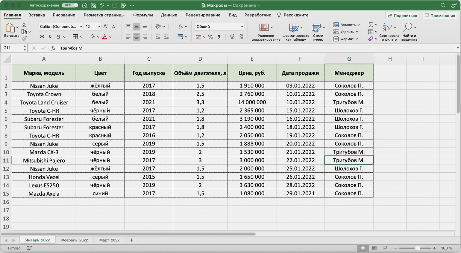
Скриншот: Skillbox Media
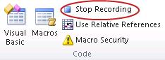
Проверяем, все ли действия с таблицей мы выполнили, и останавливаем запись макроса. Сделать это можно двумя способами:
- Нажать на кнопку записи в нижнем левом углу.
- Перейти во вкладку «Разработчик» и нажать кнопку «Остановить запись».
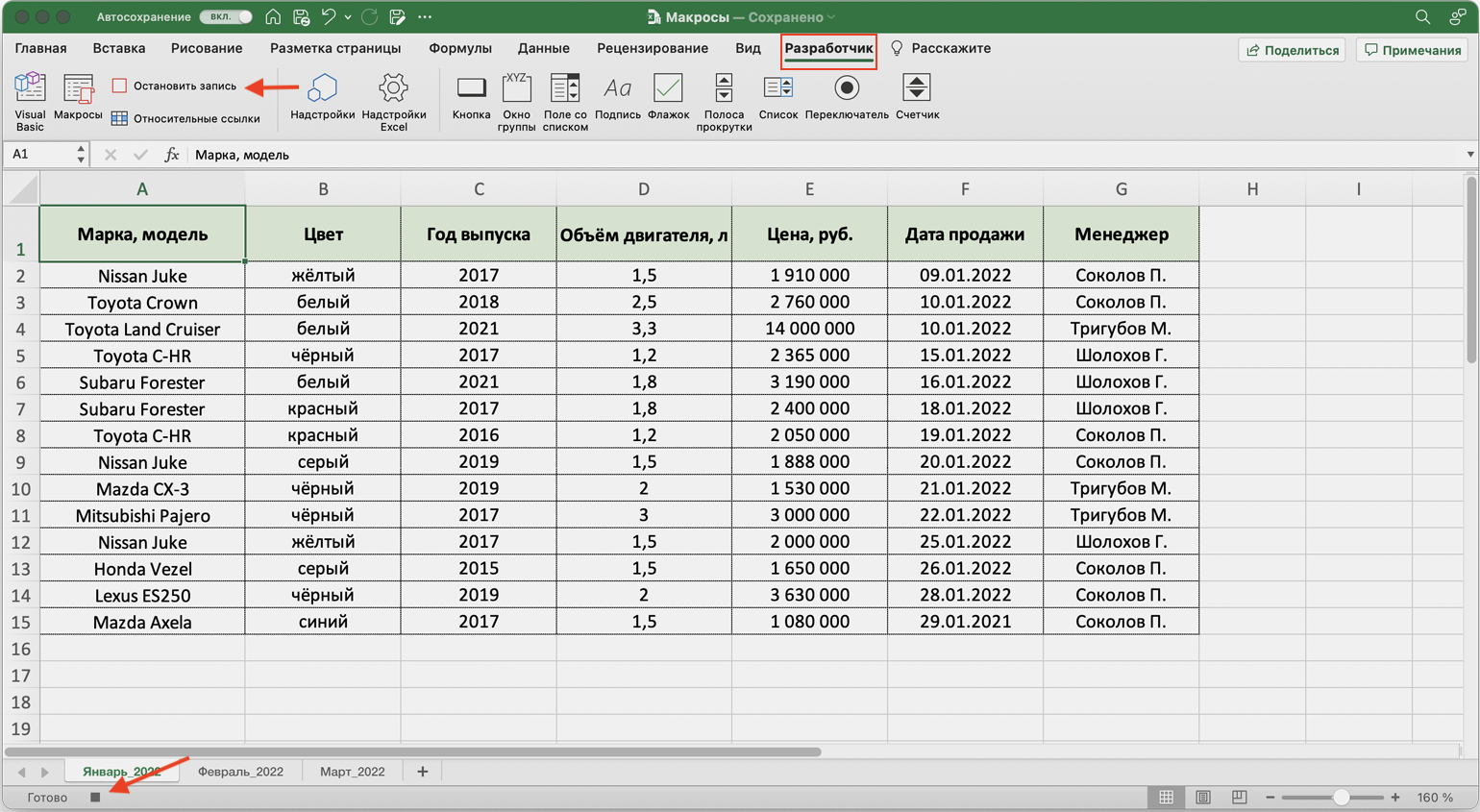
Скриншот: Skillbox Media
Готово — мы создали макрос для форматирования таблиц в границах столбцов A–G. Теперь его можно применить к другим таблицам.
Запускаем макрос
Перейдём в лист со второй таблицей «Февраль_2022». В первоначальном виде она такая же нечитаемая, как и первая таблица до форматирования.
Скриншот: Skillbox Media
Отформатируем её с помощью записанного макроса. Запустить макрос можно двумя способами:
- Нажать комбинацию клавиш, которую выбрали при заполнении параметров макроса — в нашем случае Option + Cmd + Ф.
- Перейти во вкладку «Разработчик» и нажать кнопку «Макросы».
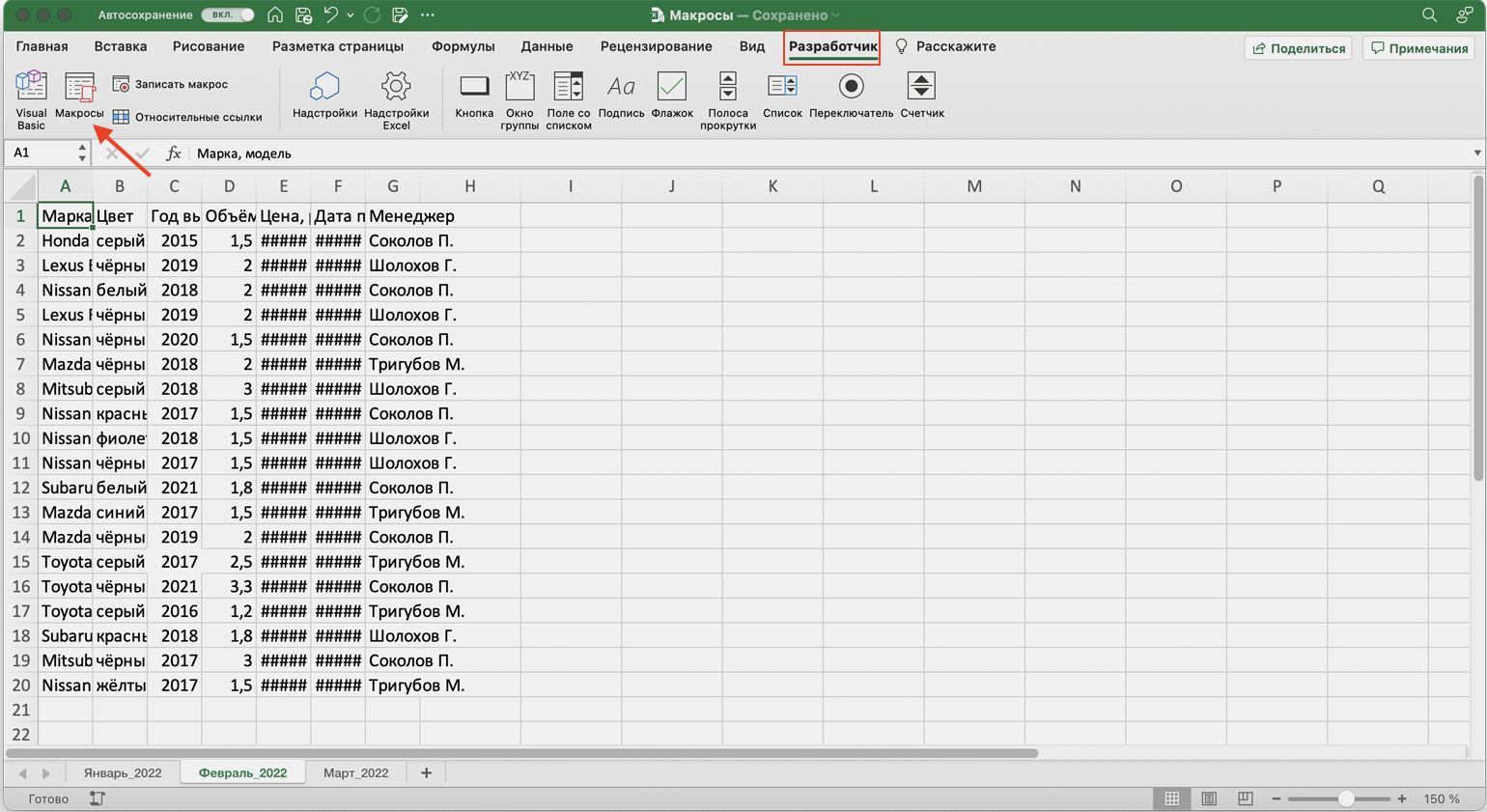
Скриншот: Skillbox Media
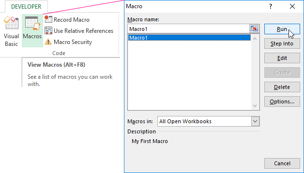
Появляется окно — там выбираем макрос, который нужно запустить. В нашем случае он один — «Форматирование_таблицы». Под ним отображается описание того, какие действия он включает. Нажимаем «Выполнить».
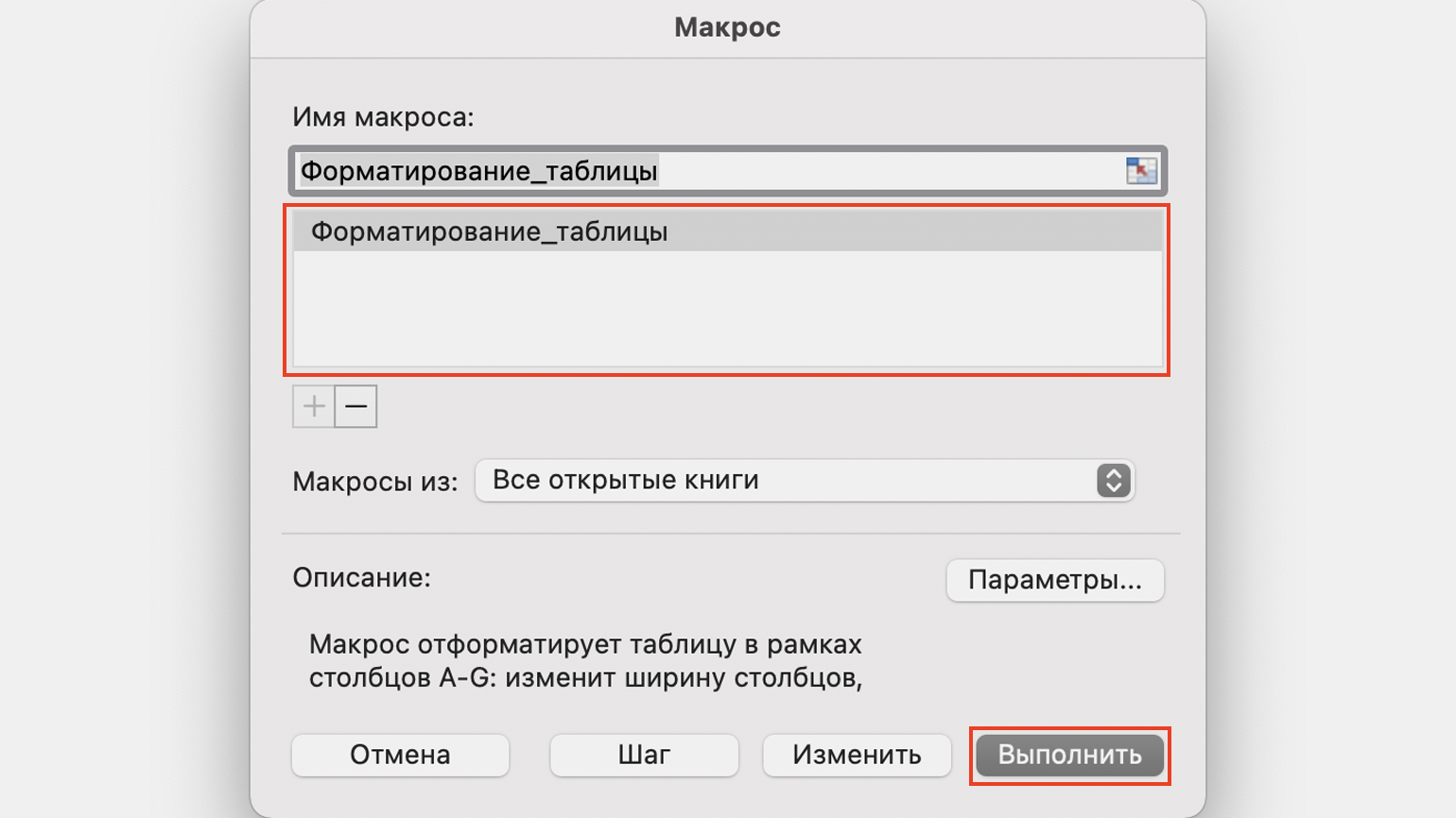
Скриншот: Skillbox Media
Готово — вторая таблица с помощью макроса форматируется так же, как и первая.
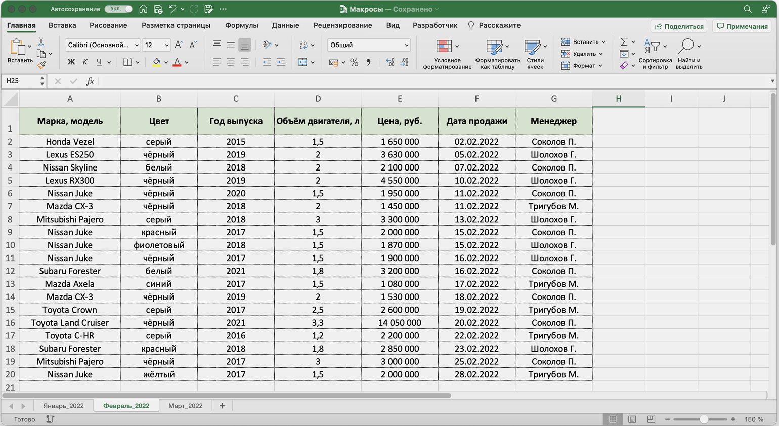
Скриншот: Skillbox Media
То же самое можно сделать и на третьем листе для таблицы продаж за март. Более того, этот же макрос можно будет запустить и в следующем квартале, когда сервис автосалона выгрузит таблицы с новыми данными.

Научитесь: Excel + Google Таблицы с нуля до PRO
Узнать больше
Using Macros in Excel allows you extending the program’s features significantly. They help turning the work of the program into an automatic process and take the majority most of the user’s routine work on themselves. You simply need learning to use Macros to increase your productivity in tens of times.
No one person recording Macros must be a specialist – a programmer. He may not know the programming VBA language when making his own Macro programs using the Macro Recorder.
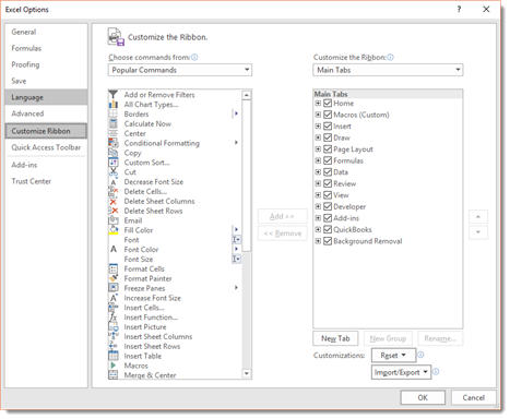
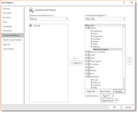
Please, enable the «DEVELOPER» panel. Just open the Options group in the File menu. In the “Excel Options” window that will be opened then, find the “Customize Ribbon” group. Pay attention to the right column of settings under the same name as “Ribbon Setup”. There tick the «DEVELOPER» tab – you can see it clearly at the photo.
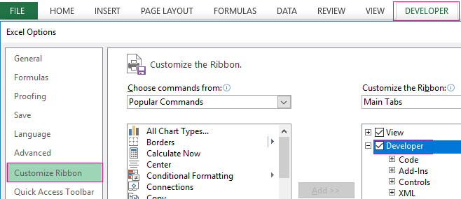
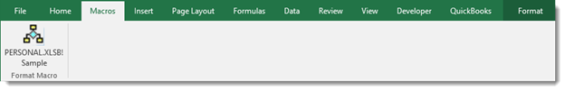
Now you have a new «DEVELOPER» tab available with all our tools for automating work in Excel and creating Macros.
Using VBA and Macros in Microsoft Excel
Macros are internal applications that always perform all the routine work, making life easier for the PC user. Each user can create a Macro even without knowledge of programming languages. To do this, use special command button runs it. In this mode, all actions of the Macro Recorder in Excel are recorded by translating the VBA code into the programming language in automatic mode. After the end of the recording, we get a ready-made program that performs the actions that the user made when writing it.
Recording Macros in Excel process
Recording Macros process is surprisingly simple. Just be extremely attentive when following these steps.
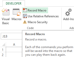
- Push Macro Recorder button on the «DEVELOPER» tab.
- When you get the dialogue window, fill it in with Macros parameters and push OK button.
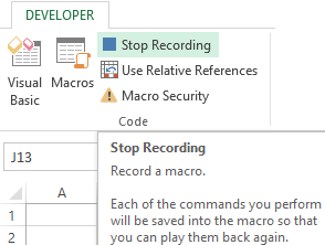
- When you finish the process, click «Stop recording» button. After this action the Macro will be automatically saved.
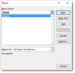
- To execute or edit the recorded Macro, pick the «Macros» button or choose ALT + F8 combination. A window with a list of recorded Macros and buttons for managing them will appear after it.
Using of Macro programs, you can increase the user’s productivity (up to dozens of times!). However, to record the user macros for 100% correctly, you must follow uncomplicated rules that significantly affect their quality at the time of recording them and performance.
Working with Macros in Excel
Follow these five simple tips, and they will help you creating Macros without programming. Take advantage of these simple recommendations that allow you to create high-quality Macro programs automatically, doing it quickly and easily.
1. Use correct names in Macros
Give your Macros short, but meaningful names. When you sympathize with the whole procedure, you will start creating many Macros. It will be easier for you finding short and meaningful names. The VBA system permits you specifying a description for the name. Be sure to always use it. The Macros name must always (!) start with letters and it cannot contain any spaces, different symbols or various punctuation marks. After the first character, you can use numbers or underscores, but the maximum name length is only eighty characters.
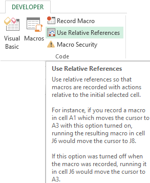
2. Use Relative and Absolute Cell References
The absolute cell reference is the exact location of the cursor when information about its location is recorded in Macro addresses with a rigid binding to a specific cell at the time of recording. Absolute references limit the capabilities of the Macros if you add or even remove data on an Excel document – the data list will become larger. Relative tools (references) do not bind the cursor to a specific cell address. Excel uses a default “Absolute” mode; however you can always change it by turning on the «Use Relative References» button located below the Macro Recorder button on the toolbar of the «DEVELOPER» tab.
3. Always start recording Macros with A1 cell position
The absolute counting of cells is always carried out from the initial (home) position A1 to the address of the cursor with your data. If you saved your Macro in the personal Macros book (we do recommend always performing it), then you can use your program on other worksheets with similar data. It never matters when you place your cursor, when you start recording a Macro. Even if it is already located in A1 cell, your first Macro must be best written after pressing Ctrl + Home keys. We will give you an example. Imagine that every month you get dozens of tables from all branches. You need organizing data and make necessary calculations for a monthly report. Performing all of these functions, record your Macro.
4. Use special direction keys when recording a Macro
Use the special “arrow” keys to control the cursor (Ctrl + Up, etc.). Using these direction keys, you can simply add, easily change or even completely delete data within the table as it is needed. Using a computer mouse for recording actions is not convenient and so much reliable. Forget about using a mouse working with Macros in Excel.
5. Create Macros for specific small tasks
Keep your Macros for small specific tasks. The more complicated code, the slower they work, especially if it is required performing many functions or calculating various formulas in a large table. When you run each process separately, you can quickly view the results to verify the accuracy of their execution. When you cannot “break” a long Macro into short units, but you want to test its functionality, do it step-by-step. Press F8 each time you want to go to the next step in the task. The process of executing the program stops when it sees an error. You can fix an error that is easy to find by debugging it or writing it in a new way.
![]()
Download Article
![]()
Download Article
This wikiHow teaches you how to enable, create, run, and save macros in Microsoft Excel. Macros are miniature programs which allow you to perform complex tasks, such as calculating formulas or creating charts, within Excel. Macros can save significant amounts of time when applied to repetitive tasks, and thanks to Excel’s «Record Macro» feature, you don’t have to know anything about programming in order to create a macro.
Things You Should Know
- Macros make it easy to automatic tasks in Microsoft Excel.
- To create macros yourself, you’ll need to enable macros in the Developer menu of Excel.
- Saving a macro-enabled spreadsheet is a little different than saving a spreadsheet without macros.
-
1
Open Excel. Double-click the Excel app icon, which resembles a white «X» on a green box, then click Blank workbook.
- If you have a specific file which you want to open in Excel, double-click that file to open it instead.
-
2
Click File. It’s in the upper-left side of the Excel window.
- On a Mac, click Excel in the upper-left corner of the screen to prompt a drop-down menu.
Advertisement
-
3
Click Options. You’ll find this on the left side of the Excel window.
- On a Mac, you’ll click Preferences… in the drop-down menu.
-
4
Click Customize Ribbon. It’s on the left side of the Excel Options window.[1]
- On a Mac, click instead Ribbon & Toolbar in the Preferences window.
-
5
Check the «Developer» box. This box is near the bottom of the «Main Tabs» list of options.
-
6
Click OK. It’s at the bottom of the window. You can now use macros in Excel.
- On a Mac, you’ll click Save here instead.


Advertisement
-
1
Enter any necessary data. If you opened a blank workbook, enter any data which you want to use before proceeding.
- You can also close Excel and open a specific Excel file by double-clicking it.
-
2
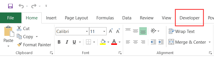
Click the Developer tab. It’s at the top of the Excel window. Doing so opens a toolbar here.
-
3
Click Record Macro. It’s in the toolbar. A pop-up window will appear.
-
4
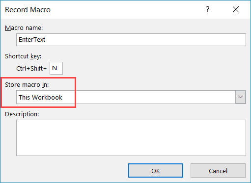
Enter a name for the macro. In the «Macro name» text box, type in the name for your macro. This will help you identify the macro later.
-
5
Create a shortcut key combination if you like. Press the ⇧ Shift key along with another letter key (e.g., the E key) to create the keyboard shortcut. You can use this keyboard shortcut to run the macro later.
- On a Mac, the shortcut key combination will end up being ⌥ Option+⌘ Command and your key (e.g., ⌥ Option+⌘ Command+T).
-
6
Click the «Store macro in» drop-down box. It’s in the middle of the window. Doing so prompts a drop-down menu.
-
7
Click This Workbook. This option is in the drop-down menu. Your macro will be stored inside your spreadsheet, making it possible for anyone who has the spreadsheet to access the macro.
-
8
Click OK. It’s at the bottom of the window. Doing this saves your macro settings and begins recording.
-
9
Perform the macro’s steps. Any step you perform between clicking OK and clicking Stop Recording while be added to the macro. For example, if you wanted to create a macro which turns two columns’ worth of data into a chart, you would do the following:
- Click and drag your mouse across the data to select it.
- Click Insert
- Select a chart shape.
- Click the chart that you want to use.
-
10
Click Stop Recording. It’s in the Developer toolbar. This will save your macro.


Advertisement
-
1
Understand why you have to save the spreadsheet with macros enabled. If you don’t save your spreadsheet as a macro-enabled spreadsheet (XLSM format), the macro won’t be saved as part of the spreadsheet, meaning that other people on different computers won’t be able to use your macro if you send the workbook to them.
-
2
Click File. It’s in the upper-left corner of the Excel window (Windows) or the screen (Mac). Doing so will prompt a drop-down menu.
-
3
Click Save As. This option is on the left side of the window (Windows) or in the drop-down menu (Mac).
-
4
Double-click This PC. It’s in the column of save locations near the left side of the window. A «Save As» window will open.
- Skip this step on a Mac.
-
5
Enter a name for your Excel file. In the «Name» text box, type in the name for your Excel spreadsheet.
-
6
Change the file format to XLSM. Click the «Save as type» drop-down box, then click Excel Macro-Enabled Workbook in the resulting drop-down menu.[2]
- On a Mac, you’ll replace the «xlsx» at the end of the file’s name with xlsm.
-
7
Select a save location. Click a folder in which you want to save the Excel file (e.g., Desktop).
- On a Mac, you must first click the «Where» drop-down box.
-
8
Click Save. It’s at the bottom of the window. Doing so will save your Excel spreadsheet to your selected location, and your macro will be saved along with it.


Advertisement
-
1
Open the macro-enabled spreadsheet. Double-click the spreadsheet that has the macro in it to open the spreadsheet in Excel.
-
2
Click Enable Content. It’s in a yellow bar at the top of the Excel window. This will unlock the spreadsheet and allow you to use the macro.
- If you don’t see this option, skip this step.
-
3
Click the Developer tab. This option is at the top of the Excel window.
- You can also just press the key combination you set for the macro. If you do so, the macro will run, and you can skip the rest of this method.
-
4
Click Macros. You’ll find it in the Developer tab’s toolbar. A pop-up window will open.
-
5
Select your macro. Click the name of the macro which you want to run.
-
6
Click Run. It’s on the right side of the window. Your macro will begin running.
-
7
Wait for the macro to finish running. Depending on how large your macro is, this can take several seconds.


Advertisement
Add New Question
-
Question
Can I use a macro that I create in other spreadsheets and future spreadsheets on the same pc?

Yes, you can use a macro that you crate in other spreadsheets and future spreadsheets on the same pc.
-
Question
How can I write macros that will change a spreadsheet as soon as I create it?
You will first need a basic understanding of VBA. There are many tutorials on this.
Ask a Question
200 characters left
Include your email address to get a message when this question is answered.
Submit
Advertisement
Video
-
Macros are generally useful for automating tasks which you must perform often, such as calculating payroll at the end of the week.
Thanks for submitting a tip for review!
Advertisement
-
Although most macros are benign, some macros can maliciously change or delete information on your computer. Never open a macro from a source which you don’t trust.
Advertisement
About This Article
Article SummaryX
1. Enable Developer options in Excel.
2. Click the Developer tab.
3. Click Record Macro.
4. Enter the macro name and details.
5. Click OK.
6. Perform the macro’s steps.
7. Click Stop Recording.
Did this summary help you?
Thanks to all authors for creating a page that has been read 710,423 times.
Is this article up to date?
Excel Macro is a record and playback tool that simply records your Excel steps and the macro will play it back as many times as you want. VBA Macros save time as they automate repetitive tasks. It is a piece of programming code that runs in an Excel environment but you don’t need to be a coder to program macros. Though, you need basic knowledge of VBA to make advanced modifications in the macro.
In this Macros in Excel for beginners tutorial, you will learn Excel macro basics:
- What is an Excel Macro?
- Why are Excel Macros Used in Excel?
- What is VBA in a Layman’s Language?
- Excel Macro Basics
- Step by Step Example of Recording Macros in Excel
Why are Excel Macros Used in Excel?
As humans, we are creatures of habit. There are certain things that we do on a daily basis, every working day. Wouldn’t it be better if there were some magical way of pressing a single button and all of our routine tasks are done? I can hear you say yes. Macro in Excel helps you to achieve that. In a layman’s language, a macro is defined as a recording of your routine steps in Excel that you can replay using a single button.
For example, you are working as a cashier for a water utility company. Some of the customers pay through the bank and at the end of the day, you are required to download the data from the bank and format it in a manner that meets your business requirements.
You can import the data into Excel and format. The following day you will be required to perform the same ritual. It will soon become boring and tedious. Macros solve such problems by automating such routine tasks. You can use a macro to record the steps of
- Importing the data
- Formatting it to meet your business reporting requirements.
What is VBA in a Layman’s Language?
VBA is the acronym for Visual Basic for Applications. It is a programming language that Excel uses to record your steps as you perform routine tasks. You do not need to be a programmer or a very technical person to enjoy the benefits of macros in Excel. Excel has features that automatically generated the source code for you. Read the article on VBA for more details.
Excel Macro Basics
Macros are one of the developer features. By default, the tab for developers is not displayed in Excel. You will need to display it via customize report
Excel Macros can be used to compromise your system by attackers. By default, they are disabled in Excel. If you need to run macros, you will need to enable running macros and only run macros that you know come from a trusted source
If you want to save Excel macros, then you must save your workbook in a macro-enabled format *.xlsm
The macro name should not contain any spaces.
Always fill in the description of the macro when creating one. This will help you and others to understand what the macro is doing.
Step by Step Example of Recording Macros in Excel
Now in this Excel macros tutorial, we will learn how to create a macro in Excel:
We will work with the scenario described in the importance of macros Excel. For this Excel macro tutorial, we will work with the following CSV file to write macros in Excel.

You can download the above file here
Download the above CSV File & Macros
We will create a macro enabled template that will import the above data and format it to meet our business reporting requirements.
Enable Developer Option
To execute VBA program, you have to have access to developer option in Excel. Enable the developer option as shown in the below Excel macro example and pin it into your main ribbon in Excel.
Step 1)Go to main menu “FILE”
Select option “Options.”


Step 2) Now another window will open, in that window do following things
- Click on Customize Ribbon
- Mark the checker box for Developer option
- Click on OK button

Step 3) Developer Tab
You will now be able to see the DEVELOPER tab in the ribbon

Step 4) Download CSV
First, we will see how we can create a command button on the spreadsheet and execute the program.
- Create a folder in drive C named Bank Receipts
- Paste the receipts.csv file that you downloaded

Step 5) Record Macro
- Click on the DEVELOPER tab
- Click on Record Macro as shown in the image below
You will get the following dialogue window

- Enter ImportBankReceipts as the macro name.
- Step two will be there by default
- Enter the description as shown in the above diagram
- Click on “OK” tab
Step 6) Perform Macro Operations/Steps you want to record
- Put the cursor in cell A1
- Click on the DATA tab
- Click on From Text button on the Get External data ribbon bar
You will get the following dialogue window

- Go to the local drive where you have stored the CSV file
- Select the CSV file
- Click on Import button
You will get the following wizard

Click on Next button after following the above steps

Follow the above steps and click on next button

- Click on Finish button
- Your workbook should now look as follows

Step 7) Format the Data
Make the columns bold, add the grand total and use the SUM function to get the total amount.

Step  Stop Recording Macro
Now that we have finished our routine work, we can click on stop recording macro button as shown in the image below

Step 9) Replay the Macro
Before we save our work book, we will need to delete the imported data. We will do this to create a template that we will be copying every time we have new receipts and want to run the ImportBankReceipts macro.
- Highlight all the imported data
- Right click on the highlighted data
- Click on Delete
- Click on save as button
- Save the workbook in a macro enabled format as shown below

- Make a copy of the newly saved template
- Open it
- Click on DEVELOPER tab
- Click on Macros button
You will get the following dialogue window

- Select ImportBankReceipts
- Highlights the description of your macro
- Click on Run button
You will get the following data

Congratulations, you just created your first macro in Excel.
Summary
Macros simplify our work lives by automating most of the routine works that we do. Macros Excel are powered by Visual Basic for Applications.
We are going to continue to explore macros in this article and learn more about creating and working with them.
Formatting with Macros
Formatting cells in workbooks can be a tedious process, especially if you have to format each worksheet in workbooks that you create. To save time and make things easier, you can use macros to format cells and worksheets simply by creating macros that do all the formatting for you. This way, you only apply the formatting once. After that, all you have to do is run the macro.
A macro can contain as many steps as you want it to contain. You can create a macro that changes the font type, color, and size, then also applies cell formatting and row and column sizes. In essence, you can create macros to do all the formatting for you.
We are going to create a macro that does the following things:
1. Changes font type, size, and color.
2. Sets a theme (under the Page Layout tab).
3. Formats the cells to Number with three decimal places.
4. Creates a table in the worksheet.
We are going to call this macro salesWorksheetFormatting.
Notice that we are storing this macro in our personal macro workbook. This way, it is available in all workbooks, and we can use it no matter what workbook we have open.
Click OK.
We can then record our macro.
Remember to stop recording when you finish all the steps involved in your macro.
Switching Between Scenarios with Macros
If we go to the Data tab, click the What-If Analysis button, then click on the Scenario Manager, we can see all the scenarios we have created.
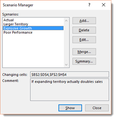
We can select any of these scenarios, then click Show to see the scenario in our worksheet.
If we want to see another scenario, we go back to the Scenario Manager, select the scenario we want to view, then click the Show button again.
This is a lot of clicks.
Instead, we can create a macro for each scenario and add a keyboard shortcut for each macro that we create. That way, we can view a scenario simply by using a keyboard shortcut.
To create a macro for a scenario, go to the Developer tab and select Record Macro.
Name the macro so that you know which scenario it is, then specify a keyboard shortcut.
You will want to store the macro in the workbook.
Click OK, then record yourself opening up the Scenario Manager, selecting a scenario, then clicking the Show button.
Stop recording when you are finished.
You can now view that scenario by running the macro.
Switching Between Custom Views with Macros
In addition to creating macros to view scenarios, you can also create macros to access custom views.
Go to the View tab and select Custom Views.
You will then see the Custom Views dialogue box.
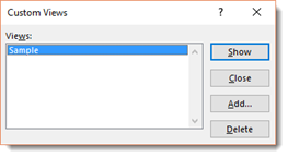
Select a custom view.
If you click the Show button, the custom view will appear in the worksheet.
Instead of having to click the View tab, click the Custom Views button, then click the Show button, you can instead create a macro with a keyboard shortcut that will do all of this for you.
To create the macro, click the Record Macro button under the Developer tab. Name the macro, then assign a keyboard shortcut to it. You will want to store the macro in the workbook.
Click OK, then record yourself going to the View tab, clicking the Custom Views button, then clicking the Show button.
Remember to stop recording when you are finished.
You can now switch to that custom view by simply running the macro.
Using Worksheet Buttons to Trigger Macros
That said, the problem with creating keyboard shortcuts to trigger macros is that, if you have a lot of macros, it can be hard to remember what keyboard shortcut triggers what macro.
Imagine having twenty macros for one workbook, then trying to remember which macro triggers cell formatting. It can be impossible and actually make things more complicated. Macros are supposed to make things easier.
Instead of creating keyboard shortcuts, you can create worksheet buttons instead.
A worksheet button is just as it sounds. It is a button that you place in your worksheet. When you click on that button, it triggers a macro.
To create a worksheet button that will trigger a macro, click in the worksheet where you want to place the button.
Go to the Developer tab. Click the Insert dropdown arrow.
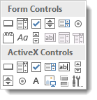
The first icon in the top left corner is a button. Click on the button icon.
Your mouse cursor now is a crosshair.
Click and drag to draw the button.
When you release your mouse, you will see the Assign Macro dialogue box.
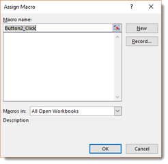
Click on the macro that you want to assign to the button.
Click OK.
The button then appears in the worksheet.
Now you can rename the button. It is recommended that you give the button the same name as the macro or a name that will remind you what the macro actually does.
You can also drag on the button handles to resize it.
When you are finished, click in the worksheet.
The button is now clickable.
Now, whenever you click on the button, it will run the macro.
Customizing Buttons and Other Shape Triggers
You can apply some customization to worksheet buttons and other shape triggers.
To apply customization, select the button. To do this, you will have to right click on it. If you just left click on it, it will run the macro. Instead, right click on it, then select one of the options in the context menu.
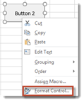
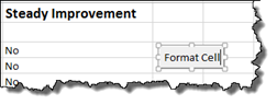
We are going to select Format Control.
This brings up the Format Control dialogue box.
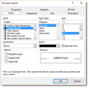
You can click through the tabs to apply different formatting options to your button.
-
The Font tab gives you options to format the text on your button.
-
The Size tab allows you to change the size of the button.
-
The Alignment tab allows you to align the text on the button.
-
The Protection tab allows you to lock an item or lock the text.
-
The Properties tab allows you to control the positioning of the button.
-
The Margins tab allows you to set margins inside the button.
-
The Alt Text tab shows you the label for the button.
Apply any formatting that you want using this dialogue box, then click OK when you are finished.
If you noticed, the one thing you could not change was the color of the button. When we go to the Developer tab to insert a button, we are left with very few formatting choices. For example, grey is the only color of button we can insert, and it is always going to be either a square or rectangle shape.
If we want to use buttons that have different colors and styles – or even use other shapes as buttons, we need to first create a shape and format it.
Click the Insert tab, then go to Shapes. Select the shape that you want to use, then drag to draw it on your worksheet as we have done below.
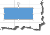
We have chosen to use a rectangle. However, you can use any shape. It does not have to be a rectangle.
The Drawing Tools Format tab is now open on the Ribbon.

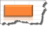
Apply a shape style to the shape if you want. You can also change the shape fill and outline colors. In addition, you can add effects such as a drop shadow.
Our shape is shown below.
Next, right click on the shape and choose Assign Macro.
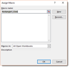
Select the macro that you want to assign to the shape, then click OK.
That macro is then assigned to the button. Whenever you click the button, the macro will be triggered.
Now, right click on the button and choose Edit Text. Add a text label to the button so you know which macro will be triggered when you click on it.
Assign a Macro to a Ribbon Icon
You can also add buttons to the ribbon that will trigger macros. To do this, first go to File>Options.
Click the Customize Ribbon tab on the left hand side of the Excel Options dialogue box.
From the Choose Commands From dropdown menu (where it currently says Popular Commands), choose Macros.
You can now see your macros.
Go to the Customize the Ribbon section of the Excel Options dialogue box. This is on the ride side of the dialogue box.
Choose the tab where you want to place your macros by clicking on it. Do not uncheck the other tabs. This will cause them to not appear on your ribbon.
We are going to choose the Home tab.
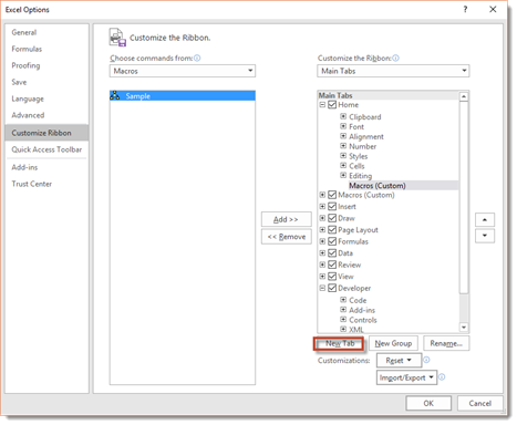
Click on the Home tab to see the groups that are currently under the Home tab. You will have to place your macros in a group under the Home tab. However, you can’t place the button in an existing group.
Instead, you have to click the New Group button, as pictured below.
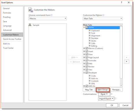
You will then see New Group (Custom), as highlighted below.
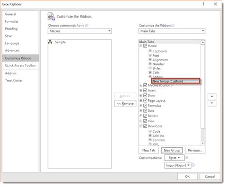
Make sure New Group (Custom) is selected.
Next, click the Rename button that appears to the right of the New Group button.
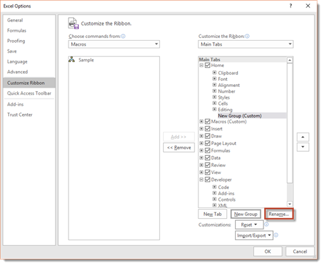
You will then see the Rename dialogue box.
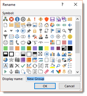
Rename the group. We are naming ours Macros.
Click OK.
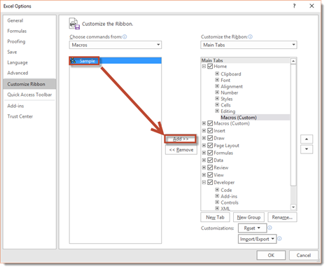
Now, select the macro that you want to add to the group. You will select it from the field on the left, then click the Add button that is between the two fields.
Click the Rename button again.
Click on a symbol to represent the macro. You can also rename it if you want.
Click OK.
When you have added all your macros and selected symbols, you can click OK to leave the Excel Options dialogue box.
Take a look at your Home tab. You can see our new Macros group to the far right on the ribbon.
NOTE: Typically, you will want to use macros that are stored in your personal macro workbook for this. That way, whenever you open Excel, those macros are on your Ribbon and available to you.
Creating Your Own Tab on the Ribbon
In addition to adding macros to an existing tab, such as Home as we did in the last section, you can also create your own tab just for your macros.
To do this, go back to File>Options>Customize Ribbon.
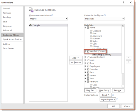
Click New Tab, as shown below.
Our new tab is then visible.
Click the Rename button, as we did in the last section.
Name your new tab, then click OK.
Now you can name the group that is included in the tab by default. Right now, its name is New Group.
You can also add more groups by clicking the New Group button.
Next, add macros to the group.
When you are finished, click OK.
You can then see the Macros tab in the Ribbon.
If we click on the Macros tab, we can see our group.
Editing Macro Code
We do not recommend that you ever attempt to edit the Visual Basic code for your macros. However, just in case you ever need to, we will show you the basics that you need to know in order to be able to make minor changes.
Just be warned, anything outside of the basic editing that we will teach you is a task best left for experienced programmers and not for the typical Excel user. If you mess up the code, you will require the assistance of a programmer to fix it, or you will have to re-record the macro.
To view and edit macro code, go to the Developer tab and click the Macros button.
Select the macro that you want to view and edit, then click the Edit button.
NOTE: If you are going to edit code in a macro that is stored in your personal macro workbook, you will need to unhide the workbook first.
Once you click the Edit button, this is what you will see:
The macro code is shown below.

At the top you see Sub Sample. Sub is for subrooting. Then you see the name of your macro.
At the end you can see that the subrooting is ended. It says End Sub.
Everything in between Sub and End Sub are instructions that the macro will carry out.
Any line where you see an apostrophe at the beginning, followed by green text, are comments. They are not actionable code. You can add more comments if you want. This is very basic, and you are not going to hurt anything by doing this.
Now let’s look at the actual code, which is anything in black font that is between Sub and End Sub.
You will see that some of the code appears between quotation marks, such as «Record a macro with a relative reference.» This is actually the text that appears in our worksheet when we run the macro. If you want, you can edit text that appears between quotation marks. Again, this is easy enough, and you do not do any damage.
Other things that may appear in your macro that you can easily change are:
-
Font type. Just type in a new font type, such as Arial.
-
Font size. Enter a new font size, such as 14.
-
True/False arguments. You can change an argument from True to False, then vice versa.
-
Range. If the range is .Range(«A1»), you could change it to another cell, such as A2.
-
Active Cell. Right now, the active cell appears as ActiveCell.FormulaR1C1. R1C1 stands for row one column one. You could change this to R2C2, for example.
If you recognize anything else and feel comfortable changing it, then you can try to do it. Just remember that you may damage the macro in the process and be forced to re-record it.
When you are finished, simply X out of the window by clicking the X in the top right corner. You do not need to do anything to save the changes. You can then run the macro whenever you want.
Adding a Confirmation Box to a Macro
Although it is not advisable that you attempt to edit the code for your macros, there is a circumstance when you will be required to edit that code. If you want to add a confirmation box to a macro, you will have to edit the code in order to create that box.
A confirmation box is a box that will ask you if you are sure that you want to run a specified macro. This is especially helpful to have if you create a macro that deletes cells or data.
Let’s show you how to do this.
Go to the Developer tab and click on the Macros button.
Select a macro for which you want to create a confirmation box, then click the Edit button.
You will then see your code.

To create the confirmation box, we need to start out by adding an If statement. Click at the beginning of the first line of code. Push the spacebar a few times. Then, click to put the cursor above the first line of code. The next snapshot will show you what we mean.
Once you have done that, we can start to enter the code.
The first thing we type is «if» then add a space, then type «msgbox» to create the confirmation box.
Add an opening bracket, as shown below. We are then told what we need to enter next, as shown below.
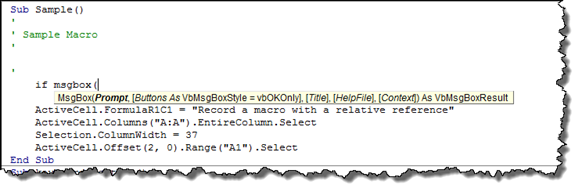
The first thing to enter is a prompt. This is the text that a user will see in the confirmation box that asks them a question.
Type in that question. Any text that will appear inside the confirmation box goes in quotes.
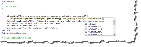
We have customized our prompt to our macro, but your prompt can be anything you need it to be.
Next, select the buttons. We want Yes and No, so we scroll down in the button dropdown menu.
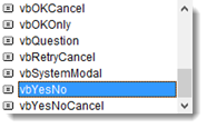
Double click on the button you want to add. It will appear in your IF statement. Add a comma after it.
Next, you can add an optional title to your dialogue box. We are going to enter «Warning.»
You do not need the rest of the parameters for a confirmation box.
Add a closing bracket to your IF statement.
We highlighted our IF statement in the snapshot below.
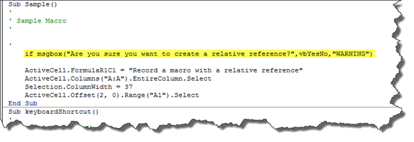
Next, add an equal sign after your closing bracket.
You will see another dropdown menu.
Double click on VBYes in the dropdown menu. This lets Excel know to display the confirmation box. If the answer clicked on in the confirmation box is YES, then to run the macro.
Add a space, then type «then.»
Press Enter.
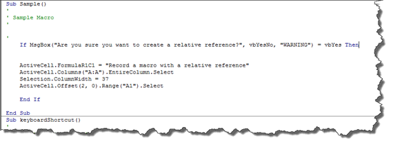
Next, at the end of your macro, but before the End Sub, type «End If» as we have done above.
Press Enter.
You can now X out of the code window.
Go ahead and run the macro for which you created the confirmation box.
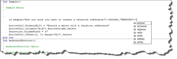
You will see the confirmation box appear on your screen. It will read, «Are you sure you want to create a relative reference?»
We are going to click Yes.
When you click Yes, the macro runs.
Macros allow automating repetitive tasks in Microsoft Excel. Some tasks need to be performed multiple times and repetition of all the actions would consume time. In these scenarios, Macros helps in automating these tasks.
A macro is a set of actions that we can run as many times as required to perform a particular task. When a macro is created, the whole mouse clicks, and the keystrokes get recorded.
For example: suppose for every month, a report is to be created for all the teachers of a school. As it is a repetitive task, macros can come into action here.
How to Record a Macro?
The following steps can be performed to record a macro in Excel:
- Click on the Developer Tab in the ribbon.

- In the Code Group, the tool Record Macros is located. Click on it.

- As macros are selected, a dialog box is opened which contains the following options to fill.

In the dialog box, enter the name of the macro in Macro name. However, space cannot be used in the Macro name to separate the words, underscore(_) can be used for this purpose. Example: Macro_name.
There are some other options also in the dialog box, i.e, where to store the macro in, the shortcut key which can be used to activate the macro, and the description for the macro created. They can be filled accordingly.
- After filling the dialog box, click on OK.
- As soon as OK is clicked, Excel Macro is recording the set of operations the user is practicing.
- Once, the work is done, in the Developer Tab, an option “Stop Recording” can be seen. Clicking on which the recording gets stopped and the created macro is saved.

How to Run the Macro?
There are different methods by which a macro can run. Some of the methods are discussed here in this article.
1. Run the Macro by Clicking on a Shape
It is one of the easiest ways to run a macro is to create any shape in the worksheet and use it for running the macro.
The steps that need to be followed are:
- Click on the Insert Tab on the ribbon.

- Go to the Illustrations group and click on the Shapes icon. In the sheet, choose any shape we like and want it to be assigned as the macro.


- Click where you want to add the shape in the sheet and the shape will automatically get inserted.

- The shape can be resized or re-formatted accordingly to the way you want. Text can also be added in the shape.

- Then Right-Click on the shape and a dialog box would be opened. Then click on Assign Macro.

- After right-clicking on the shape, another dialog box of Macro would be opened.

- In the dialog box, select the macro from the list you want to assign to your shape and click the OK button.
The work is done! Now the shape would work as a button and whenever you click on it, it will run the assigned macro.
2. Run Macro By Clicking a Button
While the shape is something you can format and play with it, a button has a standard format. A macro can also be assigned to a button for easy use and then can run the macro by simply clicking that button.
The steps that need to be followed are:
- Go to the Developer Tab on the ribbon.
- In the Controls group, click on the Button tool.

- Now, click anywhere on the Excel sheet. As soon as you do this, the Assign Macro dialog box would be opened.

- Select the macro you want to assign to that button and fill in the other options. Then click on OK.
- After that, a rectangular button can be seen on the sheet and ready to be used.

The button which appears on the sheet has default settings, and you can’t format it like the color, shape of the button.
However, the text which appears on the button can be changed. Just a right-click on the button and a dialog box would open.

Click on Edit Alt Text and change the text.
3. Run a Macro from the Ribbon (Developer Tab)
If you have multiple macros in the workbook defining different tasks, you can see a list of all the macros in the Macros dialogue box and it makes it easy to run multiple macros from a single list.
The steps that need to be followed are:
- Go to the Developer Tab on the ribbon.
- Then in Code Group, click on the Macros Tool.

- A dialog box would be opened containing the list of all the macros created in that particular workbook.

- Select that Macro that you want to run.
- Click Run.
4. Run a Macro from the VB Editor
If the user and creator of the macros are the same, then instead of spending time creating buttons and shapes, we can directly run the macro from the VB Editor.
Here are the steps:
- Go to the Developer Tab on the ribbon.
- In the Code Group, click on Visual Basic and a new window would be opened.

- Then click on the Run Macro sign, it will open a dialog box listing all the macros of that workbook.

- Select the macro you want to run from the list and click Run.

As soon as Run is clicked, the macro would be executed on the excel-sheet.
If you can only see the VB Editor window and not the sheet, then you may not see the changes happening in the worksheet. To see the changes, minimize/close the VB Editor window.
Several other features of Macros can be explored.
What is MACRO in Excel?
A macro in excel is a series of instructions in the form of code that helps automate manual tasks, thereby saving time. Excel executes those instructions in a step-by-step manner on the given data. For example, it can be used to automate repetitive tasks such as summation, cell formatting, information copying, etc. thereby rapidly replacing repetitious operations with a few clicks.
There are two methods to create the macros – The first is when you can record the macro, where Excel records every step automatically and then repeats it. The second is coding with VBAVBA code refers to a set of instructions written by the user in the Visual Basic Applications programming language on a Visual Basic Editor (VBE) to perform a specific task.read more, which requires good subject knowledge
Before recording a macro, the user has to activate the Developer tab in Excel. The Developer tabEnabling the developer tab in excel can help the user perform various functions for VBA, Macros and Add-ins like importing and exporting XML, designing forms, etc. This tab is disabled by default on excel; thus, the user needs to enable it first from the options menu.read more is a built-in option in Excel to create macros, generate VBA applications, design forms, import or export XML files, etc. Since it is disabled in Excel by default, it has to be enabled before creating and recording the macrosRecording macros is a method whereby excel stores the tasks performed by the user. Every time a macro is run, these exact actions are performed automatically. Macros are created in either the View tab (under the “macros” drop-down) or the Developer tab of Excel.
read more.
Table of contents
- What is MACRO in Excel?
- Enable the Developer tab
- Examples of Macros in Excel
- Example #1
- Example #2
- Adding the Macro Button
- How to View the Code of Macros?
- Creating Macro by Writing VBA Code
- How to Save the Recorded Macro in Excel?
- How to Enable “Macro Security Settings”?
- Frequently Asked Questions (FAQs)
- Recommended Articles
Let us learn the method to enable the Developer tab in Excel.
Enable the Developer tab
Below are the steps to activate the Developer tab in the Excel toolbar.
- Click on “options” in the File menu (as shown in the succeeding image).

- On clicking the “options”, the “Excel options” window will pop up.

- Select “customize ribbon” in the “Excel options” which provides a list of options in a dialog box.
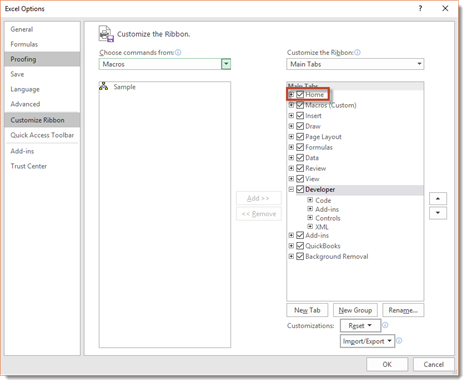
Under “customize the ribbon”, select “main tabs”. Among the list of checkboxes, select “developer” and click “ok”.
- The worksheet displays the Developer tab, as highlighted in the succeeding image.

- The user can view options like “visual basic”, “macros”, “record macro”, etc. on the ribbon of Developer tab (as displayed in the image below).


Examples of Macros in Excel
Let us understand how to add macros in excel with the help of the following example.
Example #1
A list of data with different names is available in the table below. Some names have “.” symbol. We want to replace the “.” symbol with “_” by using macros in Excel.
You can download this Macro Excel Template here – Macro Excel Template

The steps to add an excel macro are listed as follows:
- Click the “record macro” option in the Developer tab.

- The “record macro” window will pop out. Name the macro “ReplaceDot” in the “macro name” box. To assign a keyboard shortcutAn Excel shortcut is a technique of performing a manual task in a quicker way.read more, type “Ctrl+q” in the “shortcut key” box.
Select the option “This Workbook” in the “store macro in” box, which will ensure the macro is stored in the particular workbook.
It is optional to fill the “description” box explaining the task. Finally, click the “ok” button.

- The “ReplaceDot” macro will start recording the user actions in Excel. The user will observe the “stop recording” button appearing in the Developer tab.

- Let us now start replacing the “.(dot)” in the names with “_(underscore)” by using the “find and replace” option. Enter “.” in the “find” and “ _” in the “replace” option, respectively. Then click the “replace all” button.
Note: Use the shortcut key “Ctrl+H” to use “find and replace” option.


- The “replace all” option replaces all the “.” (dots) with the “_” (underscores). The number of replacements and the resulting output is shown in the succeeding image.

- The final output is displayed in the below image.

- In the end, click the “stop recording” button on the Developer tab to stop the macro recording.
Example #2
We want to run the same task for a new list of names (displayed in the below image). We will run the macro “ReplaceDot,” created in the Developer ribbon.

- Select the “enable macro” option from the Developer ribbon to view the list of macros created in the Macro window. The users can choose and run the macros based on their requirement.
The succeeding image shows the result of macros running on the new list of names.

Adding the Macro Button
Let us assign a button to the macro instead of choosing the “enableTo enable macros simply means to run or execute a macro in a particular file in order to save the time spent on repetitive actions. To enable macros, select “enable all macros” from the “trust center” of the File tab (in the “options” button).
read more macroTo enable macros simply means to run or execute a macro in a particular file in order to save the time spent on repetitive actions. To enable macros, select “enable all macros” from the “trust center” of the File tab (in the “options” button).
read more” option.
There are many groups like Add-ins, Controls, and XML under the Developer ribbon.

- The user can choose the type of button to be created. Select the first button from “form controls” in the Controls tab.

- Drag the selected button anywhere in the Excel sheet. The “assign macro” dialogue box opens. The macros to be assigned are listed in the “macro name” box.
- Select the macro “ReplaceDot,” appearing in the list and click “ok”.

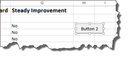
- A button appears in the worksheet. Right click the button and use “edit text” option to change the button text as “Button 3.” It is created on the right-hand side of the sheet, as shown in the below image.

- Select the new name list to implement the same task by running macros, as indicated in the previous section.

- Click the “Button 3” to run the assigned macro “ReplaceDot”.

- To change the button name, use the “edit text” option to replace the text “Button 3” with “ReplaceDot”.

Using the above steps, we can create, record, and assign the macro for various tasks and automate it.
How to View the Code of Macros?
The users can view the code for a recorded macro. Excel generates the code based on the steps carried out while recording the macro.
We can access the code using the shortcut “Alt+F11” or by editing the macro that was created earlier.
Let us view the code for the “ReplaceDot” macro using the following steps:
- Open the worksheet that contains the “ReplaceDot” macro. In the View tab, click the option “macros”. Select the “ReplaceDot” macro from the list and click the “edit” button.

- The “Microsoft Visual Basic for Applications” will be launched. The user can write or edit the code using this application. The below image shows the code of the “ReplaceDot” macro.

Creating Macro by Writing VBA Code
Before writing the VBA code, let us understand the “head” and “tail” of macros, which are the “sub” and “end sub.”

The user places the lines of VBA codes in the keyword “sub”. It executes the instructions in the code. The “end sub” keyword stops the execution of the “sub.”
Generally, there are two types of macros.
- “System Defined Function” – It performs actions like creating a link of all the worksheet names, deleting all worksheets and so on.
- “User-Defined Function” – To create a User Defined Function User Defined Function in VBA is a group of customized commands created to give out a certain result. It is a flexibility given to a user to design functions similar to those already provided in Excel.read more(UDF) in macro, the user uses the “function and end function” as the “head” and “tail” of the codes.
Note: A function returns a value, whereas the sub does not.
A macro is written on the Visual Basic EditorThe Visual Basic for Applications Editor is a scripting interface. These scripts are primarily responsible for the creation and execution of macros in Microsoft software.read more (VBE) of the “Microsoft Visual Basic for Applications”.
Let us learn the steps to write a simple macro in the VBA.
- Click the “module 1” in the “module” properties displayed on the left-hand side panel of the VBE window, and start writing the macro.

- Begin with “sub” followed by the macro name and end with “end sub”. The code is written between the “sub” and “end sub.”
The below image shows the “sub” and “end sub” for the macro named “simplemacro ( )”.
- Write code to display text in the message box. The “MsgBoxVBA MsgBox function is an output function which displays the generalized message provided by the developer. This statement has no arguments and the personalized messages in this function are written under the double quotes while for the values the variable reference is provided.read more” displays an input text message. All text in VBAText is a worksheet function in excel but it can also be used in VBA while using the range property. It is similar to the worksheet function and it takes the same number of arguments. These arguments are the values which needs to be converted.read more should be enclosed in double quotes.
For example, the code: MsgBox “Good Morning” (shown in the below image) displays the message “Good Morning” in the text box.

- The output is displayed in the succeeding image.

Hence, the same macro can be assigned buttons to automate the task.
How to Save the Recorded Macro in Excel?
After recording, the user saves the macro to reuse in any other worksheet in the future.
Let us follow the below-mentioned steps to save the macro:
- In the macro-enabled workbook, click “save as.”
- Select the “Excel macro-enabled workbook” option in the “save as type” box while saving the file.
- Finally, save the macros with the “.xlsm” file extension.

The guidelines for saving the macro names are stated as follows:
- Make sure that the name of recorded macros should start with letters (alphabets) or underscore.
- Use letters, numeric, and underscore characters.
- Avoid space, symbols, or punctuation marks.
- Maintain a maximum length of about 80 characters.
Note: When the user saves a macro’s name with space, Excel issues a warning (as shown in the succeeding image).

How to Enable “Macro Security Settings”?
In this section, let us learn to enable the “Macros security settings”.
When a user opens a workbook containing macros, a security warning – “Macros have been disabled” is displayed under the ribbon. Choose the “enable content” option in the box.

To eliminate the security warning, we need to change the “trust center settings” by using the following steps:
- Under the “trust center settings” in the File options, click “macro settings”.
- Choose the button, “Disable all macros with notification.”
- The security is enabled in the “Macro Security” of the Developer ribbon.

Note 1: The user can create absolute macros (functioning from cell A1) that help to reuse the macro in other worksheets.
Note 2: The usage of directional keys (rather than a mouse) for navigation in macros is reliable to add, delete, and change the data in the worksheet.
Frequently Asked Questions (FAQs)
1. What are macros in Excel?
Macros are a set of simple programs or instructions to automate the common and repetitive tasks performed in the Excel worksheet. It can be recorded, saved, and run multiple times as per the user’s requirement.
It is a time-saving tool involved in preparing data reports and manipulating data carried out frequently in a worksheet.
2. How to enable macros in Excel?
The users can eliminate the security warning in the worksheet and enable macros by using the following steps:
• Click “options” in the File tab.
• Select “trust center” in the “options” window.
• Choose the option “trust center settings”.
• Click “macro settings” on the left side of the navigation pane.
• Select “enable all macros” and click “ok”.
3. What is the difference between macro and VBA?
The difference between macro and VBA is stated as follows.
• Macros are programming codes that function in the Excel worksheet to perform automated and repetitive tasks. It saves the user’s time and extends the efficiency of Excel.
• Visual Basic for Applications (VBA) is a programming language of Excel used for creating macros.
Recommended Articles
This has been a tutorial to Macros in Excel. Here we discuss how to add Macros in Excel along with , along with practical examples and a downloadable template. You may also look at these useful functions in Excel –
- Excel Open XMLXML (Extensible Markup Language) is a text-based mark-up language that stores & organizes data in a human & machine-readable format. As it follows a specific script, you need to fulfill a particular set of prerequisites for importing the data into Excel or opening Excel Data into this format. read more
- VBA MacrosVBA Macros are the lines of code that instruct the excel to do specific tasks, i.e., once the code is written in Visual Basic Editor (VBE), the user can quickly execute the same task at any time in the workbook. It thus eliminates the repetitive, monotonous tasks and automates the process.read more
- MsgBox in Excel VBAVBA MsgBox function is an output function which displays the generalized message provided by the developer. This statement has no arguments and the personalized messages in this function are written under the double quotes while for the values the variable reference is provided.read more
Even if you’re a complete newbie to the world of Excel VBA, you can easily record a macro and automate some of your work.
In this detailed guide, I will cover all that you need to know to get started with recording and using macros in Excel.
If you’re interested in learning VBA the easy way, check out my Online Excel VBA Training.
What is a Macro?
If you’re a newbie to VBA, let me first tell you what a macro is – after all, I will keep using this term in the entire tutorial.
A macro is a code written in VBA (Visual Basic for Applications) that allows you to run a chunk of code whenever it is executed.
Often, you will find people (including myself) refer to a VBA code as a macro – whether it’s generated by using a macro recorder or has been written manually.
When you record a macro, Excel closely watches the steps you’re taking and notes it down in a language that it understands – which is VBA.
And since Excel is a really good note taker, it creates a very detailed code (as we will see later in this tutorial).
Now, when you stop the recording, save the macro, and run it, Excel simply goes back to the VBA code it generated and follows the exact same steps.
This means that even if you know nothing about VBA, you can automate some tasks just by letting Excel record your steps once and then reuse these later.
Now let’s dive in and see how to record a macro in Excel.
Getting the Developer Tab in the Ribbon
The first step to record a macro is to get the Developer tab in the ribbon.
If you can already see the developer tab in the ribbon, go to the next section, else follow the below steps:
The above steps would make the Developer tab available in the ribbon area.
Recording a Macro in Excel
Now that we have everything in place, let’s learn how to record a macro in Excel.
Let’s record a very simple macro – one that selects a cell and enters the text ‘Excel’ in it. I am using the text ‘Excel’ while recording this macro, but feel free to enter your name or any other text that you like.
Here are the steps to record this macro:
- Click the Developer tab.
- In the Code group, click on the Macro button. This will open the ‘Record Macro’ dialog box.

- In the Record Macro dialog box, enter a name for your macro. I am using the name EnterText. There are some naming conditions that you need to follow when naming a macro. For example, you can not use spaces in between. I usually prefer to keep my macro names as a single word, with different parts with a capitalized first alphabet. You can also use underscore to separate two words – such as Enter_Text.

- (Optional Step) You can assign a keyboard shortcut if you want. In this case, we will use the shortcut Control + Shift + N. Remember that the shortcut you assign here would override any existing shorcuts in your workbook. For example, if you assign the shortcut Control + S, you will not be able to use this for saving the workbook (instead, everytime you use it, it will execute the macro).
- In the ‘Store macro in’ option, make sure ‘This Workbook’ is selected. This step ensures that the macro is a part of the workbook. It will be there when you save it and reopen again, or even if you share it with someone.
- (Optional Step) Enter a description. I usually don’t do this, but if you’re extremely organized, you may want to add what the macro is about.
- Click OK. As soon as you click OK, it starts to record your actions in Excel. You can see the ‘Stop recording’ button in the Developer tab, which indicates that the macro recording is in progress.
- Select cell A2.
- Enter the text Excel (or you can use your name).
- Hit the Enter key. This will select cell A3.
- Click on the Stop Recording button the Developer tab.


Congratulations!
You have just recorded your first macro in Excel. You’re no longer a macro virgin.
While the macro doesn’t do anything useful, it’ll serve its purpose in explaining how a macro recorder works in Excel.
Now let’s go ahead and test this macro.
Follow the steps below to test the macro:
- Delete the text in cell A2. This is to test if the macro inserts the text in cell A2 or not.
- Select any cell – other than A2. This is to test whether the macro selects cell A2 or not.
- Click the Developer tab.
- In the Code group, click the Macros button.
- In the Macro dialog box, click on the macro Name – EnterText.
- Click the Run button.

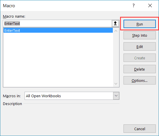
You will notice that as soon as you click the Run button, the text ‘Excel’ gets inserted into cell A2 and cell A3 gets selected.
Now, this may all happen in a split second, but in reality, the macro – just like an obedient elf – followed the exact steps you showed it while recording the macro.
So the macro first selects the cell A2, then enters the text Excel in it, and then selects the cell A3.
Note: You can also run the macro using the keyboard shortcut Control + Shift + N (hold the Control and the Shift keys and then press the N key). This is the same keyboard shortcut that we assigned to the macro when recording it.
What Recording a Macro does in the Backend
Now let’s go to the Excel backend – the VB Editor – and see what recording a macro really does.
Here are the steps to open the VB Editor in Excel:
- Click the Developer tab.
- In the Code group, click the Visual Basic button.


Or you can use the keyboard shortcut – ALT + F11 (hold the ALT key and press F11), instead of the above two steps. This shortcut also opens the same VB Editor.
Now if you’re seeing the VB Editor for the first time, don’t be overwhelmed.
Let me quickly make you familiar with the VB Editor anatomy.
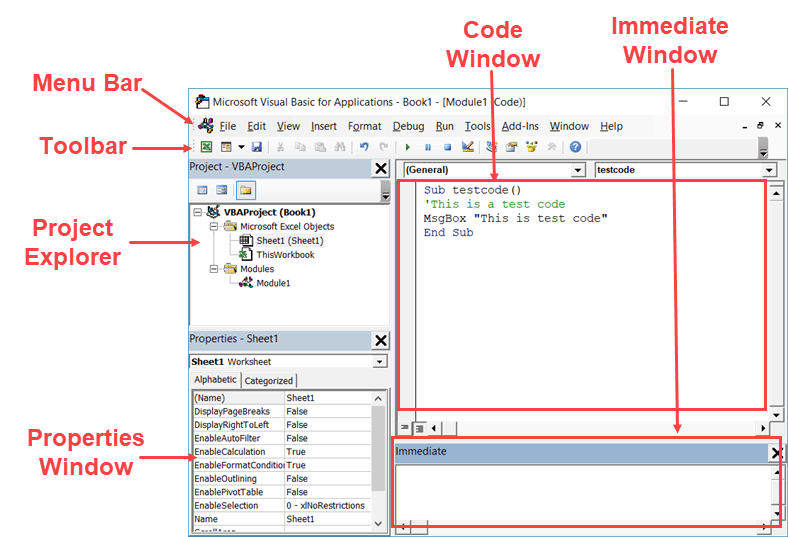
- Menu Bar: This is where you have all the options of VB Editor. Consider this as the ribbon of VBA. It contains commands that you can use while working with the VB Editor.
- Toolbar – This is like the Quick Access Toolbar of the VB editor. It comes with some useful options, and you can add more options to it. Its benefit is that an option in the toolbar is just a click away.
- Project Explorer Window – This is where Excel lists all the workbooks and all the objects in each workbook. For example, if we have a workbook with 3 worksheets, it would show up in the Project Explorer. There are some additional objects here such as modules, user forms, and class modules.
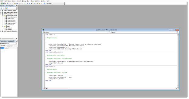
- Code Window – This is where the VBA code is recorded or written. There is a code window for each object listed in the Project explorer – such as worksheets, workbooks, modules, etc. We will see later in this tutorial that the recorded macro goes into the code window of a module.
- Properties Window – You can see the properties of each object in this window. I often use this window to name objects or change the hidden properties. You may not see this window when you open the VB editor. To show this, click the view tab and select Properties Window.
- Immediate Window – I often use the immediate window while writing code. It’s useful when you want to test some statements or while debugging. It may not be visible by default and you can make it appear by clicking the View tab and selecting the Immediate Window option.
When we recorded the macro – EnterText, the following things happened in the VB Editor:
- A new module was inserted.
- A macro was recorded with the name that we specified – EnterText
- The code was written in the code window of the module.
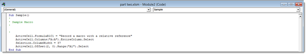
So if you double-click on the module (Module 1 in this case), a code window as shown below would appear.
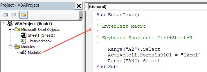
Here is the code that the macro recorder and given us:
Sub EnterText()
'
' EnterText Macro
'
' Keyboard Shortcut: Ctrl+Shift+N
'
Range("A2").Select
ActiveCell.FormulaR1C1 = "Excel"
Range("A3").Select
End Sub
In VBA, any line that follows the ‘ (apostrophe sign) is not executed. It’s a comment that’s placed for information purpose only. If you remove the first five lines of this code, the macro will still work as expected.
Now let me quickly cover what each line of code does:
The code starts with Sub followed by the name of the macro and empty parenthesis. Sub is short for Subroutine. Every subroutine (also called Procedure) in VBA starts with Sub and ends with End Sub.
- Range(“A2”).Select – This line selects the cell A2.
- ActiveCell.FormulaR1C1 = “Excel” – this line enters the text Excel in the active cell. Since we selected A2 as the first step, it becomes our active cell.
- Range(“A3”).Select – This selects cell A3. This happens as we hit the Enter key after entering the text, result of which was to select cell A3.
I hope by now you have some basic understanding of how to record a macro in Excel.
Keep in mind that the code written by a macro recorder is by no means an efficient code.
Macro recorder sometimes adds a lot of fluff to the code which is not necessary at times. But this does not mean that it’s not useful. For someone learning VBA, a macro recorder can be a great way to analyze how things work in VBA.
Absolute Vs Relative Macro Recording
You already know about absolute and relative references in Excel.. right?
If you don’t – read this tutorial on references first.
Read it? Let’s move on.
We will see later in this section on how to record macros in absolute and relative references. But before that, let me quickly summarise the difference between absolute and relative reference in VBA (in case you got lazy and didn’t read up on the link I gave a few lines ago):
If you use an absolute reference option to record a macro, the VBA code would always refer to the same cells that you used. For example, if you select cell A2, enter the text Excel and press Enter, every time – no matter where you are in the worksheet and no matter which cell is selected, your code would first select cell A2, enter the text Excel, and then move to cell A3.
If you use a relative reference option to record a macro, VBA wouldn’t hardcode the cell references. Rather, it would focus on the movement when compared with the active cell. For example, suppose you already have cell A1 selected, and you start recording the macro in the relative reference mode.
Now you select cell A2, enter the text Excel, and hit the enter key. Now, when you run this macro, it will not go back to cell A2, instead, it will move relative to the active cell. For example, if cell K3 is selected, it will move to K4, enter the text Excel, and then finally select cell K5.
Now let me tell you how to record a macro in relative references mode:
- Select cell A1.
- Click the Developer tab.
- In the Code group, click on the ‘Use Relative References’ button. It will turn green, indicating that it’s turned on.

- Click the Record Macro button.
- In the Record Macro dialog box, enter a name for your macro. I am using the name EnterTextRelRef.
- In the Store macro in option, make sure ‘This Workbook’ is selected.
- Click OK.
- Select cell A2.
- Enter the text Excel (or you can enter your name).
- Hit the Enter key. This will take the cursor to the cell A3.
- Click on the Stop Recording button the Developer tab.


This would record the macro in the relative reference mode.
Now do this.
- Select any cell (other than A1).
- Click the Developer tab.
- In the Code group, click the Macros button.
- In the Macro dialog box, click on the macro Name – EnterTextRelRef.
- Click the Run button.
What happens? Did the cursor go back to cell A3.
It wouldn’t – because you have recorded the macro in the relative reference mode. So the cursor would move relative to the active cell. For example, if you do this when cell K3 is selected, it will enter the text Excel is cell K4 and end up selecting cell K5.
Here is the code that gets recorded in the backend (VB Editor module code window):
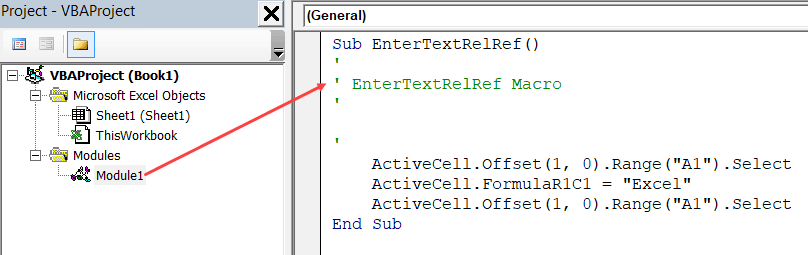
Sub EnterTextRelRef()
'
' EnterTextRelRef Macro
'

'
ActiveCell.Offset(1, 0).Range("A1").Select
ActiveCell.FormulaR1C1 = "Excel"
ActiveCell.Offset(1, 0).Range("A1").Select
End Sub
Note that this entire code doesn’t refer to the cells K3 or K4 anywhere. Instead, it uses the Activecell to refer to the selected cell and Offset to move relative to the active cell.
Don’t worry about Range(“A1”) part that the code has. It is one of those unnecessary codes that the macro recorder adds that serves no purpose and can be removed. The code would work just fine without it.
‘Use Relative Reference’ button in the Developer tab is a toggle button. You can turn it off (and switch back to absolute reference) by clicking it.
What a Macro Recorder Cannot Do
Macro recorder is great at following you in Excel and recording your exact steps, but it may fail you when you need it to do more.
- You can’t execute a code without selecting the object. If you want the macro recorder to go to the next worksheet and highlight all the filled cells in column A, without leaving the current worksheet, then it won’t be able to do this. It’s because if I ask you to do this, even you won’t be able to do that (without leaving the current sheet). And if you can’t do it yourself, how will the macro recorder capture your actions. In such cases, you need to manually go and create/edit the code.
- You can’t create a custom function with a macro recorder. With VBA, you can create custom functions that you can use in the worksheet as regular functions. You can create this by writing the code manually.
- You can’t run codes based on Events: In VBA you can use many events – such as opening a workbook, adding a worksheet, double-clicking on a cell, etc, to run a code associated with that event. You can use a macro recorder to do this.
- You can’t create loops with a macro recorder. When you manually enter the code, you can leverage the power of loops in VBA (such as For Next, For Each Next, Do While, Do until). But you can’t do this when you record a macro.
- You can’t analyze conditions: You can check for conditions within the code using macro recorder. If you write a VBA code manually, you can use the IF Then Else statements to analyze a condition and run a code if true (or another code if false).
- You can’t pass arguments in a macro procedure: When you record a macro, it will never have any arguments. A subroutine can take input arguments that can be used within the macro to perform a task. While recording a macro, this can not be done as the recorded macros are independent and are not connected to any other existing macros.
Macro-Enabled File Extensions
When you record a macro, or you manually write VBA code in Excel, you need to save the file with a macro-enabled file extension (.xlsm).
Before Excel 2007, there was one single file format that used to suffice – .xls.
But from 2007 onwards, .xlsx was introduced as the standard file extension. The files that are saved as .xlsx cannot hold a macro in it. So if you have a file with .xlsx extension and you record/write a macro and save it, it will warn you to save it in macro-enabled format, and show you a dialog (as shown below):
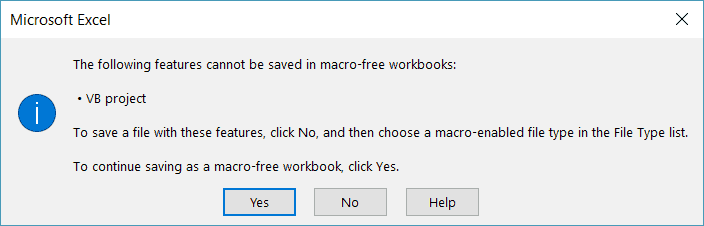
If you select No, Excel allows you to save it in a macro-enabled format. But if you click Yes, Excel will automatically remove all the code from your workbook and save it as a .xlsx workbook.
So if you have a macro in your workbook, you need to save it in the .xlsm format to keep that macro.
Different Ways to Run a Macro in Excel
So far, we have seen only one way to run a macro in Excel – which is using the Macro dialog box.
But there are a number of ways you can run macros.
- Run a Macro from the Ribbon (Developer Tab)
- Using a keyboard shortcut (which you have to assign)
- Assign the Macro to a Shape
- Assign the Macro to a Button
- Run a Macro from the VB Editor
Conclusion – Record a Macro when Stuck
I already mentioned that a macro recorder is a useful tool for anybody working with VBA in Excel.
As you use the macro recorder a few times, you will notice that it spits out a lot of unnecessary code. However, it’s still useful and gives you some ideas on where to start. For example, if I ask you to filter a column of cells using VBA, and you have no idea what the syntax is, you can quickly record a macro and check out the code.
A macro recorder is an indispensable tool and even after years of VBA coding experience under my belt, I often resort to the macro recorder for help.
You May Also like the Following Excel Tutorials:
- How to Sort Data in Excel using VBA (A Step-by-Step Guide)
- How to Create and Use an Excel Add-in
- Excel Personal Macro Workbook | Save & Use Macros in All Workbooks
- How to Use Excel VBA InStr Function (with practical EXAMPLES)
- Working with Cells and Ranges in Excel VBA
- Working with Worksheets in Excel VBA
- Working with Workbooks in Excel VBA
- Creating a User Defined Function in Excel using VBA
- Excel VBA Events – The Easy Guide.
- How to Enable Macros in Excel?