
Перейти к содержанию
На чтение 1 мин Опубликовано 04.06.2015
Если вы открываете одни и те же документы каждый день, сохраните их в качестве рабочей области. Когда вы запустите файл рабочей области, Excel откроет все нужные документы, запомнив расположение окон. Это позволит значительно сэкономить время.
- Для начала откройте два или более документа.
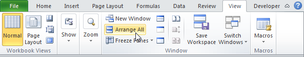
- На вкладке View (Вид) выберите команду Arrange All (Упорядочить все).

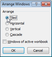
- Определите желаемый параметр расположения документов на экране. Например, Tiled (Рядом).
- Нажмите ОК.
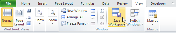
- На вкладке View (Вид) нажмите Save Workspace (Сохранить рабочую область).
- Сохраните файл рабочей области (.xlw) в папку на компьютере.
- Закройте Excel.
- Откройте файл рабочей области.
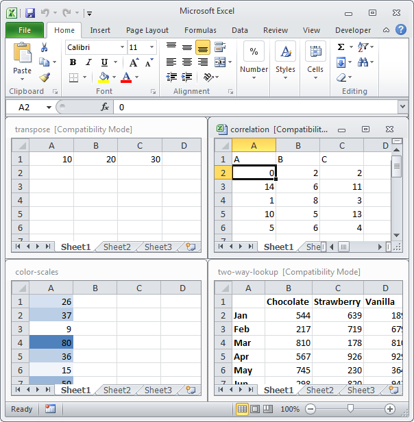
Результат:

Примечание: Сам по себе файл рабочей области не содержит документов. Поэтому вам нужно сохранить каждую книгу индивидуально, если вы вносили в неё какие-либо изменения. Кроме того, если вы измените местоположение документа, Excel не сможет запустить его при открытии файла рабочей области.
Оцените качество статьи. Нам важно ваше мнение:
If you’ve ever opened a Microsoft Excel workbook to find no columns, rows and/or scrollbars, this is probably why: The workbook’s author hid some portion of the Excel worksheet from view so users can focus on the working area without distractions. When it looks like everything is missing, it’s often because the owner of the document has disabled properties and options to protect the working area.
SEE: The Complete Microsoft Office Master Class Bundle (TechRepublic Academy)
In this tutorial, I’ll show you how to inhibit several worksheet properties and options so user focus stays on the working area. This process is easy to implement and takes very little time. I’m using Microsoft 365 Desktop on a Windows 10 64-bit system, but you can also use older versions. Excel’s online version lets you turn off gridlines and the heading rows.
You can download the Microsoft Excel demo file for this tutorial.
Jump to:
- Why hide unused areas in Excel?
- Hiding columns and rows in Excel
- Hiding the header rows and formula bar in Excel
- Hiding the sheet tabs in Excel
- Restoring your original display
- Moving toward Excel’s protection feature
Why hide unused areas in Excel?
You usually hide a column or row to conceal or protect data and formulas, so you might be wondering why anyone would want to hide everything else. The reason? Hiding everything but the working area is a good way to obscure data and formulas you don’t want users to see or try to change.
Another good reason to hide unused areas is to make your worksheet function similarly to dashboards, which are growing in popular use. Viewers, or end consumers, might click around to focus on something in the sheet or to filter a report or graph like they would in a dashboard, but they won’t be able to make changes to the underlying data. When you’re trying to make your Excel worksheet function like a dashboard, you won’t want to see many of Excel’s traditional sheet elements.
SEE: 30 Excel tips you need to know (TechRepublic Premium)
Whether you’re protecting data or removing distractions, hiding white space and other areas of the worksheet can help. However, hiding parts of the worksheet comes with one inherent behavior that’s difficult to work around: Hiding rows and columns displaces the work area. For instance, if you hide all unused rows and columns, the work area will end up in the top-left corner of the sheet rather than the middle.
That might not matter for your particular use case, but in case it does, we’ll cover a second method that allows you to center the work area by turning off the gridlines. Keep in mind that many of the tips we’re covering today, including the hidden gridlines tip, actually involve inhibiting the display of some sheet properties and turning things off rather than truly hiding anything.
Hiding columns and rows in Excel
Hiding unused columns and rows within the sheet is a good way to keep users from exploiting the space and/or keep them focused on relevant information. It’s also a great way to spiff up a dashboard so it looks professional and complete.
SEE: The best keyboard shortcuts for rows and columns in Microsoft Excel (TechRepublic)
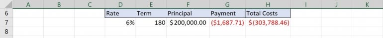
To demonstrate, we’ll use the sample worksheet shown in Figure A, which has a small working area and a lot of wasted space — unused areas that might tempt a user to wander around.
Figure A
To hide unused rows, take the following steps:
1. Click any cell in the first unused row above the work area and press Shift + Spacebar to select that row. If you’re working with the demonstration file, click a cell inside row 1.
2. Press Ctrl + Shift + Down Arrow to select every row between the selected row and the bottom of the sheet.
3. If Excel selects the header row (row 6), hold down the Shift key and press the Up Arrow to remove row 6 from the selection.
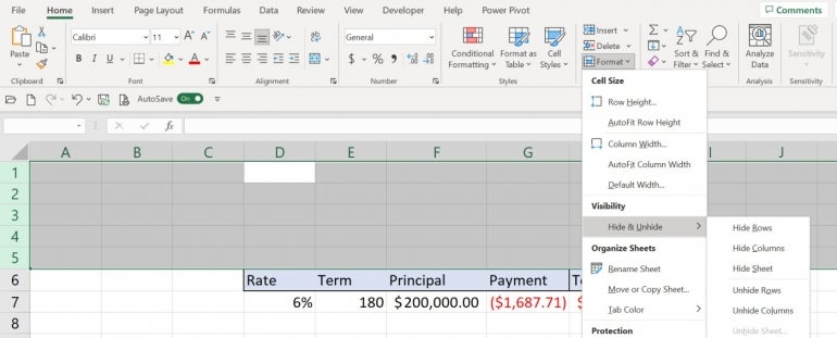
4. Click the Home tab.
5. In the Cells group, click the Format dropdown and choose Hide & Unhide. Then, choose Hide Rows (Figure A) or right-click the selection and choose Hide from the resulting submenu. You could also simply press Ctrl + 9.
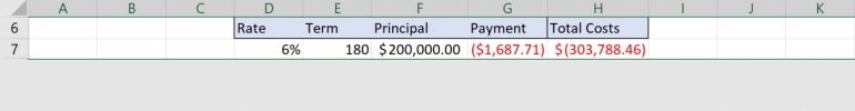
Hiding the unused rows above the work area moves the work area to the top of the sheet, as shown in Figure B. This is the displacement issue I mentioned earlier.
Figure B
Repeat the steps above to select all the rows below the work area. Begin by clicking a cell in row 8. Figure C shows the results.
Figure C
Now it’s time to hide all of the unused columns:
1. Click any cell in column A.
2. Press Ctrl + Down Arrow to select the entire column, or click the header cell to select the entire column.
3. Press Ctrl + Shift + Down to add columns B and C to the selection.
4. If Excel selects the first column in the work area, hold down the Shift key and press the Left Arrow key to remove it from the selection.
5. In the Cells group, click the Format dropdown and choose Hide & Unhide, and then choose Hide Columns. You can also right-click the selection and choose Hide from the resulting submenu or simply press Ctrl + 0.
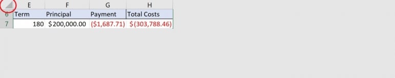
Repeat the process above by first clicking any cell in column I. Figure D shows the results. As you can see, the work area is now in the top-left corner of the screen. You can’t easily access the hidden rows and columns if you choose to make changes.
Figure D
To unhide all columns and rows in the sheet, click the sheet selector at the intersection of the row and column header cells. Doing so will select the entire sheet. Press Shift + Ctrl + 9 and Shift + Ctrl + 0 to quickly unhide everything.
How to inhibit columns and rows in Excel
If the displacement that occurred in our previous examples won’t work for what you need, you can seemingly hide empty rows and columns by inhibiting other sheet elements, such as gridlines.
To inhibit the view of the gridlines in Excel, do the following:
1. Click the View menu.
2. In the Show group, uncheck Gridlines (Figure E).
Figure E
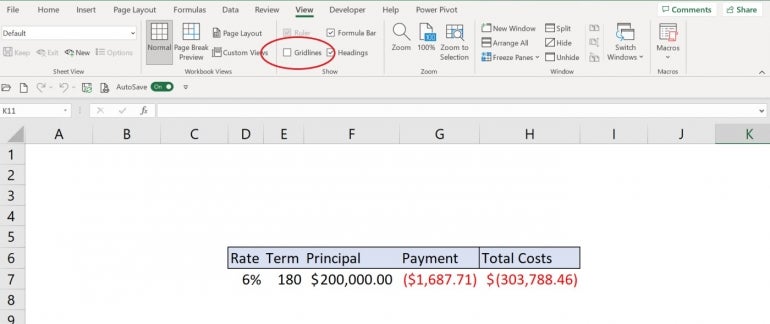
The gridlines are gone. This simple visual change will help the viewer move straight to the work area and stay there. Admittedly, it’s still white space, but the absence of the gridlines is a good start. However, the view still displays a few other sheet elements that you might want to inhibit. Next, let’s look at hiding header rows and the formula bar.
Despite the absence of gridlines, the window still looks like an Excel sheet. Inhibiting the view of the header rows and the formula bar will tone down the “this is an Excel sheet, wander around and do whatever you like” mindset and keep users in the working area.
For this part of our tutorial, you’ll turn off both header rows and the formula bar the same way you did the gridlines. Click the View tab and then uncheck Formula Bar and Headings in the Show group. Figure F shows the results.
Figure F
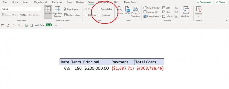
At this point, users with limited Excel skills probably won’t make any effort to wander beyond the working area.
You can still select the header cells even though you can’t see them. If you want to add or delete columns or rows, you still can. In Figure F, you can see that I inserted a column and a couple of rows to better center the work area.
For better or worse, the Formula bar is an application-level property. The next Excel file you or your users open will do so with the Formula bar turned off. For that reason, you might not want to turn it off, especially if users won’t know how to turn it back on.
Hiding the sheet tabs in Excel
The sheet tabs provide quick access to other sheets within the same Excel document. If you don’t want to see them, you can inhibit these sheet tabs as well. To turn off the display of sheet tabs, follow these steps:
1. Click the File tab.
2. In the left pane, click Options.
3. In the left pane, click Advanced.
4. In Display Options For This Workbook, uncheck the first three options (Figure G). You might as well turn off the scroll bars while you’re at it, too.
Figure G
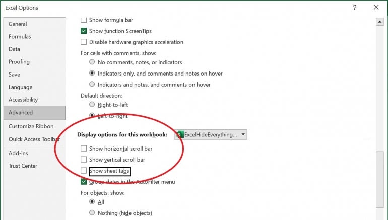
5. Click OK.
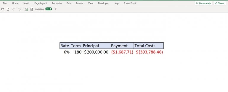
You can toggle the ribbon, but most likely, the file will open with the ribbon exposed. This is another application-level setting that you really can’t control from one use to another.
At this point, you’re done. Figure H shows a simple sheet with few distractions.
Figure H
Restoring your original display
You’ve made a lot of changes, but all of them are easy to implement and to reset. You can complete this entire reset in under five minutes. To restore the display, simply repeat the instructions listed above in reverse.
Moving toward Excel’s protection feature
If you decide that you must inhibit the Formula bar and the ribbon, you should use the WorkBook_Open() Sub procedure. This procedure will run its code when the user opens the workbook. Then, you can turn them back on using the Before_Close() Sub procedure.
What we’ve done throughout this tutorial is a simple bit of illusion. Sometimes that will be enough, and frankly, it looks nice. However, nothing in this article protects any of the sheet’s cells. For that, you’ll want to use Excel’s protection feature.
To learn more about Excel protection, read the following articles:
- Five tips for working with Excel sheet protection (TechRepublic)
- How to protect Excel formulas (TechRepublic)
- How to use passwords to grant users access to different Microsoft Excel workbook ranges (TechRepublic)
Do you have other Microsoft questions or functions that you want to learn more about? TechRepublic has thousands of Microsoft tutorials and resources available to help you make the most of your Microsoft technologies. We also offer a variety of Microsoft education programs and certifications through TechRepublic Academy.
What Is A Worksheet?
A worksheet is a collection of cells where all your data and formulas are stored. Each cell can contain either data (numeric or text) or a formula.

Cells are arranged in rows and columns in the workbook. Rows are labelled with numbers going from 1 at the very top to 1,048,576 at the very bottom. Columns are labelled with letters going left to right starting with A and going to XFD. Since there are only 26 letter in the alphabet, the column label convention starts with A to Z for the first 26 columns, then moves onto AA, AB,…, AZ, BA, BB,… until we get to ZZ and the process starts again at AAA and goes on until the 16,384 th column which is labelled XFD. The intersection of a column and a row is a cell and the address of this cell is given by its column letter and row number.
One cell in the worksheet is called the active cell. This means you can edit its contents or enter new data or formula into the cell by typing on your keyboard. You can identify the active cell in the worksheet by:
- A thick dark green border around the cell.
- The associated column and row will be a darker shade of gray.
- The cell’s address will appear in the Name Box.
Selecting A Worksheet
By default a new Excel workbook contains 3 worksheets, but you can change the default number of sheets in a new workbook to any number you like.
Only one worksheet is visible at a time, this is called the active worksheet. Select a different sheet by clicking on it from the sheet tabs at the bottom of the workbook, or use the Ctrl + Page Up and Ctrl + Page Down keyboard shortcuts to scroll through all the sheets in the workbook.
Renaming A Worksheet
The default names Excel gives worksheets are pretty generic (Sheet1, Sheet2, Sheet3 etc…) but you can change them to something more meaningful, so if your sheet contains sales data you might name it Sales Data.
Rename a worksheet.
- Right click on the sheet which you want to rename.
- Select Rename from the menu. Type your new name then press Enter.
You can also rename a worksheet by double left clicking on the sheet tab.
Deleting A Worksheet
Delete a worksheet.
- Right click on the sheet which you want to delete.
- Select Delete from the menu.
You can also delete a worksheet from the Home tab in the Cells section by going to Delete then Delete Sheet.
Inserting A Worksheet
Insert a worksheet.
- Right click on any sheet.
- Select Insert from the menu.
- Alternatively, press the small plus sign icon to the right hand side of all the sheets.
You can also insert a worksheet from the Home tab in the Cells section by going to Insert then Insert Sheet.
Moving A Worksheet
You can move sheets around to arrange them into any order you like.
Left click on the sheet which you want to move, hold the mouse button down and drag the sheet to the desired location. A small sheet icon will display on your cursor while you are dragging the sheet to its new location.
Moving or Copying a Worksheet
For more options like moving a sheet to another workbook or making a copy of the sheet, use the Move or Copy command from the right click menu.
Move or Copy a worksheet.
- Right click on the sheet which you want to move or copy.
- Select Move or Copy from the menu.
- If you want to move or copy the sheet to a different workbook then select the workbook from the drop down menu. Note that you will only be able to choose a new workbook or a currently open workbook from the drop down menu.
- Select the location to move the sheet to.
- Check the Create a copy box to make a copy of the sheet.
- Press the OK button to make the changes.
About the Author
John is a Microsoft MVP and qualified actuary with over 15 years of experience. He has worked in a variety of industries, including insurance, ad tech, and most recently Power Platform consulting. He is a keen problem solver and has a passion for using technology to make businesses more efficient.
In this lesson, I will explore the basic parts of Microsoft Excel Window. Below is a screenshot of the startup window of the Microsoft Excel application. In this window, you can see a simple layout and icons of different commands of the Microsoft Excel 2019 window.
- Quick Access Toolbar
- File Tab
- Title Bar
- Control Buttons
- Menu Bar
- Ribbon/Toolbar
- Dialog Box Launcher
- Name Box
- Formula Bar
- Scroll Bars
- Spreadsheet Area
- Leaf Bar
- Column Bar
- Row Bar
- Cells
- Status Bar
- View Buttons
- Zoom Control

Quick Access Toolbar:
You will see this toolbar on the left-upper corner of the screen. Its purpose is to display the most frequently used commands of Excel. You can customize this toolbar based on your choice of commands.
File Tab:
In Excel 2007, it was an “Office” button. This menu does the file-related operations, i.e. create new excel documents, open an existing file, save, save as, print file, etc.
Title Bar:
The header or title bar of the spreadsheet is located at the top of the window. It presents the name of the active document.
Control buttons:
They are those symbols in the upper-right of the window that allows you to modify the labels, minimize, maximize, share and close the sheet.
Menu bar:
Under the diskette or save icon or the Excel icon (this will depend on the version of the program); labels or bars that allow modifying the sheet are displayed. These are the menu bar, and consist of a File, Insert, Page Layout, Formulas, Data, Review, View, Help, and a Search Bar with a light bulb icon. These menus have subcategories that simplify the distribution of information and analysis of calculations.
Ribbon/Toolbar:
There are a series of elements that are part of each menu bar. On the selection of any menu, a series of command options/icons will display on a ribbon. For example, if you press the “Home” tab, you will see cut, copy, paste, bold, italic, underline, etc commands. Similarly, if you click on the “Insert” tab, you will see tables, illustrations, additional, recommended graphics, graphics, and maps, among others. On the other hand, if we press the option “Formulas”. Insert functions, auto sum, recently used, finances, logic, text, date and time, etc.
Toolbar/Ribbon is a group of organized commands in three sections.
- Tabs: They are the top section of the Ribbon and contain groups of related commands. Home, Insert, Page Layout, Formula, Data, etc, are examples of ribbon tabs.
- Groups: They organize related commands; the name of each group appears below the Ribbon. For example, a group of commands related to fonts or a group of commands related to alignment, etc.
- Commands: They appear within each group as mentioned above.
Dialog Box Launcher:
This is a very small down arrow located in the lower-right corner of a command group on the Ribbon. By clicking this arrow explore more options about the concerned group.
Name box:
Show the location of the active cell, row, or column. You can make more than one selection.
Formula bar:
It is a bar that allows you to observe, insert or edit the information/formula entered in the active cell.
Scrollbars:
Those are the tools that allow you to mobilize both the vertical and horizontal view of the document. They can be activated by clicking on the internal bar of your platform, or on the arrows, you have on the sides. In addition to that, you can use the mouse wheel to automatically scroll up or down; or use the directional keys.
Spreadsheet Area:
It is the working area where you enter your data. It constitutes the entire spreadsheet with its rows, cells, columns, and built-in information. By means of shortcuts, we can carry out the activities of the toolbar or formulas of arithmetic operations (add, subtract, multiply, etc.). The blinking vertical bar called “cursor” is the insertion point. It indicates the insertion location of the typing.
Leaf Bar:
At the bottom, a text that says sheet 1 is displayed. This sheet bar explains the spreadsheet that is currently being worked on. Through this, we can alternate several sheets at our convenience or add a new one.
Columns Bar:
Columns are a series of boxes vertically organized in the entire sheet. It columns bar is located below the formula bar. The columns are listed with letters of the alphabet. Start with the letter A to Z, and then after Z, it will continue as AA, AB, and so on. The maximum limit of columns is 16,384.
Rows Bar:
It is that left part of the sheet where a sequence of numbers is expressed. Start with number one (1) and as we move the cursor down, more rows will be added. The maximum number of rows goes to 1,048,576.
Cells:
Cells are those parallelepipeds that divide the spreadsheet into several segments that allow rows to be separated from columns. The first cell of a spreadsheet is represented by the initial letter of the alphabet and the number one (A1).
Status Bar:
This bar is located at the bottom of the window and shows very important information. It also shows when something is wrong, or the document is ready to be delivered or printed.
This displays the quick calculations of the selected digits, like sum, average, count, maximum, minimum, etc.
You can configure the status bar by right-clicking on the status bar. You can insert or remove any command from the provided list.
View Buttons:
It is a group of three buttons arranged at the left of the Zoom control, close to the right-bottom of the screen. Through this, you can see three different types of excel sheet views.
- Normal view: This displays the Excel page in normal view.
- Page Layout view: This displays the exact view of Excel’s page as it will be printed.
- Page Break view: This shows the page break preview before printing.
Zoom Control:
Zoom control is located in the lower-right area of the Excel window. It allows you to ZOOM-IN or ZOOM-OUT a particular area of the spreadsheet. It is represented by magnifying icons with the symbols of maximizing (+) or minimizing (-). In the most modern versions, it consists of a segment with the icons of more, and less and an element that separates both options; which allows you to manipulate them by clicking on any of these.
On the other hand, it also explains how many times the document has been moved away or approached in percentages (%). The version of Microsoft Excel 2019, it allows you to zoom out by 10% and zoom up to 400%.
Back to Microsoft Excel Tutorial
Microsoft Excel is convenient for creating tables and doing calculations. Its working area is a set of cells to be filled with data. Consequently, the data can be formatted, used for building graphs, charts, summary reports.
For a beginner, working with tables in Excel may seem complicated at the first glance. It is differs considerably from the principles of table construction in Word. However, let us start from the very basics: creating and formatting tables. By the time you reach the end of this article, you will understand there is no better tool for creating tables than Excel.
Creating a table in Excel: a dummy’s guide
Working with Excel tables for dummies does not tolerate haste. There are different ways to create a table for a specific purpose, and each of them has its advantages. Therefore, let us start with assessing the situation visually.
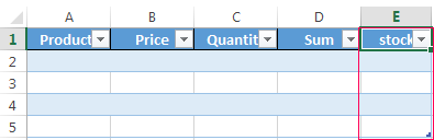
Look carefully at the work sheet of the table processor:
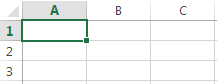
It is a set of cells in columns and rows. Essentially, it’s a table. The columns are marked with letters. The rows are designated with numbers. There are no borders.
First of all, let’s learn to work with cells, rows and columns.
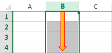
How to select a column and a row
To select the entire column, left-click on the letter that marks it.
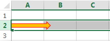
To select a row, click on the number it’s designated with.
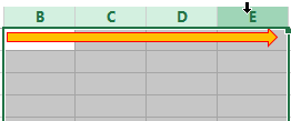
To select several columns or rows, left-click on the name, hold down the button and drag the pointer.
To select a column with the help of hot keys, place the cursor in any cell of the column and press Ctrl + Space. The key combination Shift + Space is used to select a row.
How to resize cells
If your information does not fit in the table, you need to resize the cells.
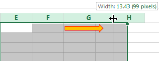
- You can move them manually by grabbing the cell boundary with the left mouse button.
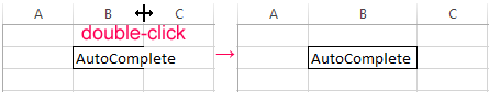
- If the cell contains a long word, you can double-click on the boundary of the column/row. The program will expand its boundary automatically.
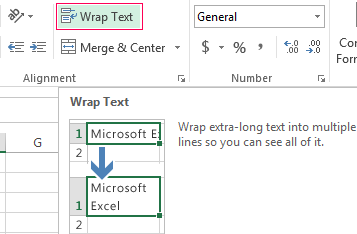
- If you need to increase the height of a row preserving the column width, use the button «Wrap Text» in the tool bar.
To change the column width and the row height in a certain range, resize 1 column/row (by dragging its boundaries manually) – and all the selected columns and rows will be resized automatically.
Important note. To go back to the previous size, you can press the «Undo Typing» button or the hot-key combination CTRL+Z. However, it works only if used immediately. Later on, it will not help.
To bring the rows to their initial boundaries, open the tool menu: «HOME»-«Format» and choose «AutoFit Row Height».
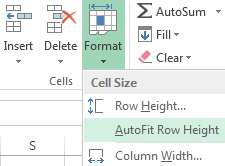
This method does not work for columns. Click «Format» — « AutoFit Row Width» Memorize this number. Select any cell in the column that needs to go back to the initial size. Click «Format» — «Column Width» again and enter the value suggested by the program (as a rule, it’s 8.43 – the number of characters in the Calibri font, size 11 pt). OK.
How to insert a column or row
Select the column/row to the right of/below the place where the insertion needs to be made. That is, the new column will appear to the left of the selected cell. The new row will be pasted above it.
Right-click on the cell and select «Insert» in the drop-down menu (or hit the hot-key combination CTRL+SHIFT+»=»).
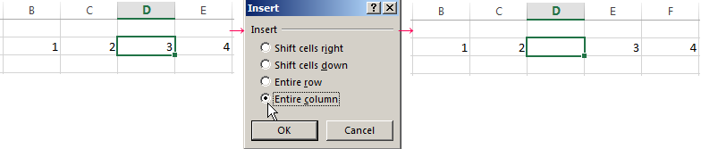
Select «Entire column» and press OK.
Hint. To insert a new column quickly, select a column in the desired position and hit CTRL+SHIFT+PLUS.
All these skills will come handy when building a table in Excel. You will need to resize the cells and insert rows/columns in the process.
Creating a table with formulas step by step
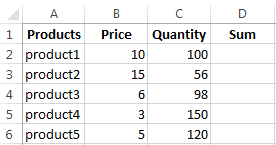
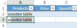
- Fill in the header manually by entering the column headings. Fill in the rows by entering your data. Apply the acquired knowledge in practice: expand the column boundaries, adjust the row height.
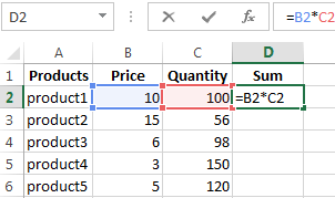
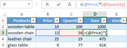
- To fill in the «Sum» column, place the cursor in its first cell. Enter «=». In such a way, we inform Excel: a formula will be here. Select the cell B2 (with the first price). Enter the multiplication symbol (*). Select the cell C2 (with the quantity). Press ENTER.
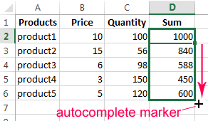
- When you hover the pointer over the cell containing the formula, a small cross will appear in its bottom right corner. It points out the autocomplete marker. Grab it with the left mouse button and drag it to the end of the column. The formula will be copied into every cell.
- Designate the boundaries of your table. Select the range containing your data. Click the button «HOME»-«Border» (on the main page in the «Font» menu). And click «All Borders».
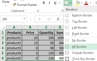
Now the column and row borders will be visible when you print the table.
The «Font» menu allows you to format the data in your Excel table the way you would do it in Word.
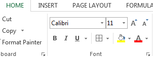
For example, change the font size and highlight the header in bold. You may also apply center alignment, word wrap, etc.
Creating a table in Excel: a step-by-step instruction
You already know the simplest way to create tables. However, Excel can offer a more convenient variant (in terms of the subsequent formatting and work with the data).
Let us construct a smart (dynamic) table:
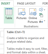
- Go to the «INSERT» tab – the «Table» tool (or press the hot-key combination CTRL+T).
- This will open a dialog window, in which you need to enter the data range. Check the box for a table with headings. Click OK. It’s no big deal if you don’t enter the proper range on the first try. The smart table is flexible, dynamic.
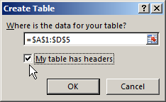
Important note. You can also take an alternative route: start with selecting the range of cells, then press the «Table» button.
Now enter your data into the ready framework. If you need an additional column, place the cursor in the heading cell. Make the entry and press ENTER. The range will expand automatically.

If you need additional rows, grab the autocomplete marker in the bottom right corner and drag it downward.
How to work with a table in Excel
With the release of new versions of the program, working with tables in Excel has become more interesting and dynamic. After a smart table has been formed on the spreadsheet, the tool «TABLE TOOLS» — «DESIGN» becomes available.
Here you can name the table or resize it.
Various styles are available to you, as well as the opportunity to transform the table into a regular range or a consolidated sheet.
MS Excel dynamic electronic tables offer immense opportunities. Let us begin with the basic skills of data entry and autocompletion:
- Select a cell by clicking on it with the left mouse button. Enter the text/numeric value. Press ENTER. If you need to change the value, place the cursor in the cell again and enter the new data.
- When you enter a value repetitively, Excel will recognize it. You will only need to enter several symbols and press enter.
- In a smart table, to apply a formula to the entire column, enter it in the first cell. The program will copy the formula in other cells automatically.
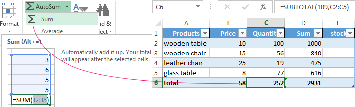
- To calculate the totals, select the column containing the values plus an empty cell for the future total and click the «Sum» button (the «Editing» tool group on the «HOME» tab, or press the hot-key combination ALT+»=»).
When you click on the little arrow to the right of every subheading in the header, you obtain access to the additional tools for working with the data in the table.
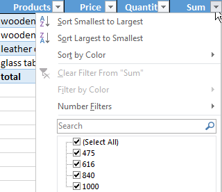
Sometimes the user has to work with huge tables, in which you need to scroll several thousand rows to see the totals. Deleting the rows is not an option (you will still need the data later). However, you can hide them. To this end, use number filters (depicted in the image above). Uncheck the values that need to be hidden.