
Содержание
- VBA Get Workbook Name in Excel
- Syntax to get current Workbook name using VBA in Excel
- Get Name of the Active Workbook using VBA in Excel
- Macro to Get Current Workbook Name using VBA in Excel
- Instructions to Run VBA Macro Code or Procedure:
- Other Useful Resources:
- Объект Names (Excel)
- Замечания
- Пример
- Методы
- Свойства
- См. также
- Поддержка и обратная связь
- Get workbook name only
- Syntax of the CELL function
- Syntax of the MID function
- Syntax of the SEARCH function
- Get workbook name only
- Explanation
- Get Workbook Name and Worksheet Name from a Range in Excel-VBA
- How to Reference Another Sheet or Workbook in Excel (with Examples)
- Referencing a Cell in the Same Sheet
- Referencing a Cell in the Another Sheet
- Automatically Creating Reference to Another Sheet in the Same Workbook
- How to Reference Another Workbook in Excel
- External Reference to an Open Workbook
- How to Create Reference to Another Workbook (Automatically)
- External Reference to a Closed Workbook
- Impact of Changing File Location on References
- Reference to a Defined Name (in the same or external workbook)
- Referencing the defined name in the same worksheet or workbook
- Referencing the defined name in another workbook (Open or Closed)
- How to Create Reference to a Named Range
VBA Get Workbook Name in Excel
VBA Get Workbook Name in Excel. We can return workbook name using Workbook.Name property. Here workbook represents an object. It is part of Workbooks collection. Returns a string value representing Workbook name. We can find Active Workbook or Current Workbook name using Name property of Workbook.
Syntax to get current Workbook name using VBA in Excel
Here is the following syntax to get the Name of the Workbook using VBA in Excel.
Where expression: It represents Workbook object which is part of workbooks collection.
Name: It represents property of Workbook object to get Workbook name.
Get Name of the Active Workbook using VBA in Excel
Let us see the following example macro to get current or active workbook name in using VBA in Excel. Where ‘Name’ represents the property of Workbook object. It helps to get the name of the Workbook.
Output: Please find the output screenshot of the above macro code.
 Active Workbook Name
Macro to Get Current Workbook Name using VBA in Excel
Here is another example macro code to get current workbook name using VBA in Excel.
Output: Here is the output screenshot of the above macro code.
 This Workbook Name
Instructions to Run VBA Macro Code or Procedure:
You can refer the following link for the step by step instructions to execute VBA code or procedure.
Other Useful Resources:
Click on the following links of the useful resources. These helps to learn and gain more knowledge.
Источник
Объект Names (Excel)
Коллекция всех объектов Name в приложении или книге.
Замечания
Каждый объект Name представляет определенное имя для диапазона ячеек. Имена могут быть встроенными именами, например базами данных, Print_Area и Auto_Open, или пользовательскими именами.
Аргумент RefersTo должен быть указан в нотации в стиле A1, включая знаки доллара ($) при необходимости. Например, если ячейка A10 выбрана на листе Лист1 и вы определяете имя с помощью аргумента RefersTo «=лист1! A1:B1», новое имя фактически относится к ячейкам A10:B10 (так как вы указали относительную ссылку). Чтобы указать абсолютную ссылку, используйте «=лист1!$A$1:$B$1».
Пример
Используйте свойство Names объекта Workbook , чтобы вернуть коллекцию Names . В следующем примере создается список всех имен в активной книге, а также адресов, на которые они ссылаются.
Используйте метод Add , чтобы создать имя и добавить его в коллекцию. В следующем примере создается новое имя, которое ссылается на ячейки A1:C20 на листе с именем Sheet1.
Используйте name (index), где index — это номер индекса имени или определенное имя, чтобы вернуть один объект Name . В следующем примере имя mySortRange удаляется из активной книги.
В этом примере в качестве формулы для проверки данных используется именованный диапазон. В этом примере данные проверки должны быть на листе 2 в диапазоне A2:A100. Эти данные проверки используются для проверки данных, введенных на листе Sheet1 в диапазоне D2:D10.
Методы
Свойства
См. также
Поддержка и обратная связь
Есть вопросы или отзывы, касающиеся Office VBA или этой статьи? Руководство по другим способам получения поддержки и отправки отзывов см. в статье Поддержка Office VBA и обратная связь.
Источник
Get workbook name only
Excel allows us to obtain the workbook name of the file we are working on, by using the CELL , MID and SEARCH functions. The CELL function provides information about a cell such as the cell’s address, format or contents. The MID function extracts a substring from the middle of a string while the SEARCH function returns the starting position of a substring within a string. This step by step tutorial will assist Excel users in getting only the workbook name of an Excel file.
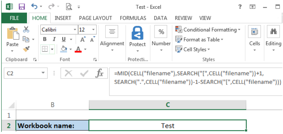 Figure 1. Final result : Get the workbook name of the Excel file “Test”
Final formula: = MID(CELL(«filename»),SEARCH(«[«,CELL(«filename»))+1,SEARCH(«.»,CELL(«filename»))-1-SEARCH(«[«,CELL(«filename»)))
Syntax of the CELL function
- info_type – a text which specifies the type of information about the cell that we want to obtain; allowed values are: address, col (for column), color, contents, filename, format, parentheses, prefix, protect, row, type, width
- reference – optional ; the cell that we want to obtain information about; if omitted, the reference cell is the cell that was last modified
Syntax of the MID function
- text – the text string containing the substring we want to obtain
- start_num – the position of the first character of the substring we want to obtain
- num_chars – the number of characters we want MID to return
Syntax of the SEARCH function
= SEARCH ( find_text , within_text , [ start_num ])
- find_text – the substring that we want to find
- within_text -the text string where we will search for the value of the find_textargument
- start_num – optional ; the position of the character in the within_text argument where we want to start searching
Get workbook name only
We want to get only the name of the workbook.
This is the working formula using the CELL, MID and SEARCH functions:
=MID(CELL(«filename»),SEARCH(«[«,CELL(«filename»))+1, SEARCH(«.»,CELL(«filename»))-1-SEARCH(«[«,CELL («filename»)))
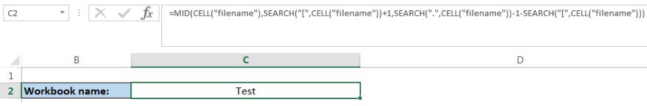 Figure 2. Entering the formula to get the workbook name
To apply the formula, we follow these steps:
- Select cell C2
- Insert the formula: = MID ( CELL («filename»), SEARCH («[«, CELL («filename»))+1, SEARCH («.», CELL («filename»))-1- SEARCH («[«, CELL («filename»)))
- Press enter
 Figure 3. Result for the workbook name: “Test”
The formula returns the workbook name: “Test”.
Explanation
=MID(CELL(«filename»),SEARCH(«[«,CELL(«filename»))+1, SEARCH(«.»,CELL(«filename»))-1-SEARCH(«[«,CELL («filename»)))
To understand the formula, we divide the MID formula into three segments.
First segment : CELL («filename»)
Second segment: SEARCH («[«, CELL («filename»))+1
Third segment: SEARCH («.», CELL («filename»))-1- SEARCH («[«, CELL («filename»))
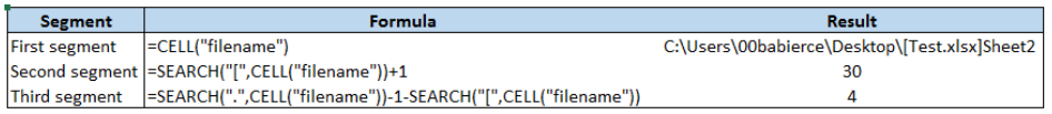 Figure 4. Arguments for the MID formula to get the workbook name
Remember that the syntax for the MID function is:
- The first segment serves as the text – which returns the cell filename C:Users0babierceDesktop[Test.xlsx]Sheet2
- The second segment is the argument for start_num – the position of the first character of the workbook name “Test” ; in this case, start_num is 30 or the 30th character of the cell filename
- The third segment is the argument for num_chars – the number of characters we want MID to return, which is 4 (Test has 4 characters)
Most of the time, the problem you will need to solve will be more complex than a simple application of a formula or function. If you want to save hours of research and frustration, try our live Excelchat service! Our Excel Experts are available 24/7 to answer any Excel question you may have. We guarantee a connection within 30 seconds and a customized solution within 20 minutes.
Источник
Get Workbook Name and Worksheet Name from a Range in Excel-VBA
I have a bit of code now that prompt the user to select a range (1 area, 1 column, several rows). This is the code where it prompt the user to do so:
How can I however get the Workbook name and Worksheet name from the above selection?
- Workbook name of destination wb — this I have achieved but using cmd: ThisWorkbook (before prompting the user to do anything)
Worksheet name of destination ws — this would preferbly also be read from above code, where it prompt the user with «Set Rng /—/»
Workbook name of source wb — after reading the destination ws, I want to promt the user with a Open-dialuge to select the source Workbook, where I will promt the user to select an additional range (source range) — which will be input to 3 & 4.
Worksheet name of source ws — see 3
Also preferrbly I would like to have the absolute ws name ‘Sheet1’ etc. not what it is named to (e.g. Kalle Anka).
EDIT: I know it in the input-dialouge show if another ws or wb is selected than from where the macro was initiated, i.e. ‘[Cognos Orders and deliveries.xlsx]Truck Orders’!$F$11:$F$18. But if I dim Set as Range — is there any way to retrive that info? If it were a String you could maybes split the String with ! and then ] to get the ws and wb seperately? How now with a Range?
EDIT2: Based on answers below, I’ve tried this with following result/problem:
At these 2 last rows I get Error.
- Run error nr ’91’? It says that objectvariable or With-blocvariabel has not been designated
Источник
How to Reference Another Sheet or Workbook in Excel (with Examples)
To be able to reference cells and ranges is what makes any spreadsheet tool work. And Excel is the best and most powerful one out there.
In this tutorial, I will cover all that you need to know about how to reference cells and ranges in Excel. Apart from the basic referencing on the same sheet, the major part of this tutorial would be about how to reference another sheet or workbook in Excel.
While there is not much difference in how it works, when you reference another sheet in the same file or reference a completely separate Excel file, the format of that reference changes a bit.
Also, there are some important things you need to keep in mind when referencing another sheet or other external files.
But worry… nothing too crazy!
By the time you’re done with this tutorial, you will know all there is to know about referencing cells and ranges in Excel (be in the same workbook or another workbook).
Let’s get started!
This Tutorial Covers:
Referencing a Cell in the Same Sheet
This is the most basic level of referencing where you refer to a cell on the same sheet.
For example, if I am in cell B1 and I want to refer to cell A1, the format would be:
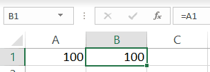
When you do this, the value in the cell where you use this reference will be the same as that in cell A1. And in case you make any changes in cell A1, these would be reflected in the cell where you have used this reference.
Referencing a Cell in the Another Sheet
If you have to reference another sheet in the same workbook, you need to use the below format:
First, you have the sheet name followed by an exclamation sign which is followed by the cell reference.
So if you need to refer to cell A1 in Sheet 1, you need to use the following reference:
And if you want to refer to a range of cells in another sheet, you need to use the following format:
So, if you want to refer to the range A1:C10 in another sheet in the same workbook, you need to use the below reference:
Note that I have only shown you the reference to the cell or the range. In reality, you would be using these in formulas. But the format of the references mentioned above are going to remain the same
In many cases, the worksheet you refer to would have multiple words in the name. For example, it could be Project Data or Sales Data.
In case you have spaces or non-alphabetical characters (such as @, !, #, -,etc.), you need to use the name within single quotes.
For example, if you want to refer cell A1 in the sheet named Sales Data, you will use the below reference:
And in case the name of the sheet is Sales-Data, then to refer to cell A1 in this sheet, you need to use the below reference:
When you refer to a sheet in the same workbook, and then later change the name of the worksheet, you don’t need to worry about the reference breaking down. Excel will automatically update these references for you.
While it’s great to know the format of these references, in practice, it’s not such a good idea to manually type these every time. It would be time-consuming and highly error-prone.
Let me show you a better way to create cell references in Excel.
Automatically Creating Reference to Another Sheet in the Same Workbook
A much better way to create cell reference to another sheet is to simply point Excel to the cell/range to which you want to create the reference and let Excel create it itself.
This will ensure that you don’t have to worry about the exclamation point or quotes being missing or any other format issue cropping up. Excel will automatically create the correct reference for you.
Below are the steps to automatically create a reference to another sheet:
- Select the cell in the current workbook where you need the reference
- Type the formula till you need the reference (or an equal-to sign if you just want the reference)
- Select the sheet to which you need to refer to
- Select the cell/range that you want to refer to
- Hit Enter to get the result of the formula (or continue working on the formula)
The above steps would automatically create a reference to the cell/range in another sheet. You will also be able to see these references in the formula bar. Once you’re done, you can simply hit the enter key and it will give you the result.
For example, if you have some data in cell A1:A10 in a sheet named Sales Data, and you want to get the sum of these values in the current sheet, following will be the steps:
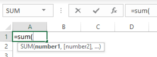
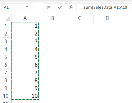
- Type the following formula in the current sheet (where you need the result): =Sum(

- Select the ‘Sales Data’ sheet.
- Select the range that you want to add (A1:A10). As soon as you do this, Excel will automatically create a reference to this range (you can see that in the formula bar)
- Hit the enter key.
When you’re creating a long formula, you may need to refer to a cell or a range in another sheet, and then have a need to come back to the origin sheet and refer to some cell/range there.
When you do this, you will notice that Excel automatically inserts a sheet reference to the sheet where you have the formula. While this is alright and doesn’t harm, it’s not needed. In such a case, you can choose to keep the reference or remove it manually.
Another thing you need to know when creating references by selecting the sheet and then the cell/range is that Excel will always create a relative reference (i.e., references with n0 $ sign). This means that if I copy and paste the formula (one with reference to another sheet) in some other cell, it would automatically adjust the reference.
Here is an example that explains relative references.
Suppose I use the following formula in cell A1 in current sheet (to refer to cell A1 in a sheet name SalesData)
Now, if I copy this formula and paste in cell A2, the formula will change to:
This happens because the formula is relative and when I copy and paste it, the references will automatically adjust.
In case I want this reference to always refer to cell A1 in the SalesData sheet, I will have to use the below formula:
The dollar sign before the row and column number lock these references so that these don’t change.
Here is a detailed tutorial where you can learn more about absolute, mixed, and relative references.
Now that we have covered how to reference another sheet in the same workbook, let’s see how we can refer to another workbook.
How to Reference Another Workbook in Excel
When you refer to a cell or a range to another Excel workbook, the format of that reference would depend on whether that workbook is open or closed.
And of course, the name of the workbook and the worksheets also play a role in determining the format (depending on whether you have spaced or non-alphabetical characters in the name or not).
So let’s see the different formats of external references to another workbook in different scenarios.
External Reference to an Open Workbook
When it comes to referring to an external open workbook, you need to specify the workbook name, the worksheet name, and the cell/range address.
Below is the format you need to use when referring to an external open workbook
Suppose you have a workbook ‘ExampleFile.xlsx’ and you want to refer to cell A1 in Sheet1 of this workbook.
Below is the reference for this:
In case there are spaces in the external workbook name or the sheet name (or both), then you need to add put the file name (in square brackets) and the sheet name in single quotes.
Below are the examples where you would need to have the names in single quotes:
How to Create Reference to Another Workbook (Automatically)
Again, while it’s good to know the format, it’s best not to type it manually.
Instead, just point Excel in the right direction and it will create these references for you. This is a lot faster with way fewer chances of errors.
For example, if you have some data in cell A1:A10 in a workbook named ‘Example File’ in the sheet named ‘Sales Data’, and you want to get the sum of these values in the current sheet, following will be the steps:
- Type the following formula in the current sheet (where you need the result): =Sum(
- Go to the ‘Example File’ workbook
- Select the ‘Sales Data’ sheet.
- Select the range that you want to add (A1:A10). As soon as you do this, Excel will automatically create a reference to this range (you can see that in the formula bar)
- Hit the enter key.
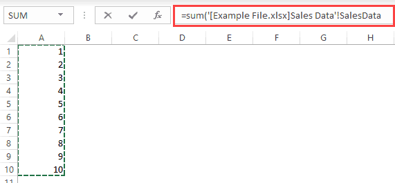
This would instantly create the formula with the correct references.
One thing you would notice when creating a reference to an external workbook is that it will always create absolute references. This means that there is a $ sign before the row and column numbers. This means that if you copy and paste this formula to other cells, it would keep referring to the same range due to absolute reference.
In case you want this to change, you need to change the references manually.
External Reference to a Closed Workbook
When an external workbook is open and you refer to this workbook, you just need to specify the file name, sheet name, and the cell/range address.
But when this is closed, Excel has no clue where you look for the cells/range you referred to.
This is why when you create a reference to a closed workbook, you also need to specify the file path.
Below is a reference that refers to cell A1 in the Sheet1 worksheet in the Example File workbook. Since this file is not open, it also refers to the location where the file is saved.
The above reference has the following parts:
- File Path – the location on your system or network where the external file is located
- File Name – the name of the external workbook. This would include the file extension as well.
- Sheet Name – the name of the sheet in which you are referring to the cells/ranges
- Cell/Range Address – the exact cell/range address to which you’re referring
When you create an external reference to an open workbook and then closed the workbook, you would notice that the reference automatically changes. After the external workbook is closed, Excel automatically inserts a reference to the file path as well.
Impact of Changing File Location on References
When you create a reference to a cell/range in an external Excel file and then close it, the reference now uses the file path as well.
But then if you change the file location, nothing is going to change in your workbook (in which you create the reference). But since you have changed the location, the link has now been broken.
So if you close and open this workbook, it will tell you that the link is broken and you need to either update the link or break it completely. It will show you a prompt as shown below:
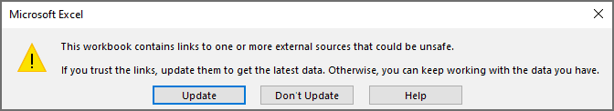
When you click on Update, it will show you another prompt where you can choose the options to edit the links (which will show you the below dialog box)
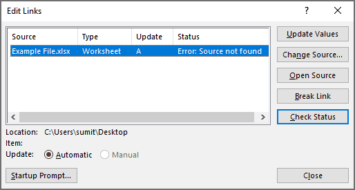
If you need to keep these files linked, you can specify the new location of the file by clicking on Update Values. Excel opens a dialog box for you where you can specify the new file location by navigating there and selecting it.
Reference to a Defined Name (in the same or external workbook)
When you have to refer to cells and ranges, a better way is to create defined names for the ranges.
This is helpful as it makes it easy for you to refer to these ranges using a name instead of a long and complicated reference address.
For example, it’s easier to use =SalesData instead of =[Example File.xlsx]Sheet1′!$A$1:$A$10
And in case you have used this defined named in multiple formulas and you need to change the reference, you need to only do it once.
Here are the steps to create a named range for a range of cells:
- Select all the cells that you want to include in the named range
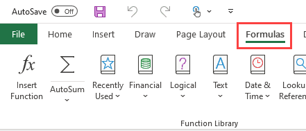
- Click the Formulas tab
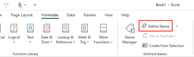
- Click on the Define Name option (it’s in the Defined Names group)
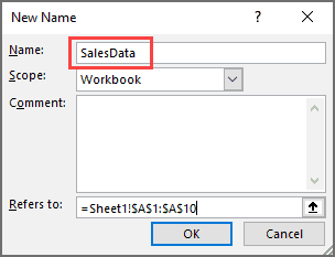
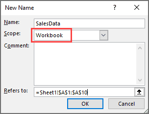
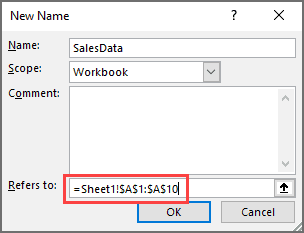
- In the New Name dialog box, give this range a name (I am using the name SalesData in this example). Remember you can’t have spaces in the name
- Keep the scope as Workbook (unless you have a strong reason to make it sheet-level)
- Make sure the Refers to the range is correct.
- Click OK.
Now your named range has been created and you can use it instead of the cell references with cell addresses.
For example, if I want to get the sum of all these cells in the SalesData range, you can use the below formula:
And what if you want to use this named range is other worksheets or even other workbooks?
You just need to follow the same format we have discussed in the above section.
No need to go back to the beginning of this article. Let me give you all the examples here itself so you get the idea.
Referencing the defined name in the same worksheet or workbook
If you have created the defined name for the workbook level, you can use it anywhere in the workbook by just using the defined name itself.
For example, if I want to get the sum of all the cells in the named range we created (SaledData), I can use the below formula:
In case you have created a worksheet level named range, you can use this formula only if the named range is created in the same sheet where you’re using the formula.
In case you want to use it on another sheet (say Sheet2), you need to use the following formula:
And in case there are spaces or alphanumeric characters in the sheet name, you will have to put the sheet name in single quotes.
Referencing the defined name in another workbook (Open or Closed)
When you want to reference a named range in another workbook, you will have to specify the workbook name and then the name of the range.
For example, if you have an Excel workbook with the name ExampleFile.xlsx and a named range with the name SalesData, then you can use the below formula to get the sum of this range from another workbook:
In case there are spaces in the file name, then you need to use these in single quotes.
In case you’ve sheet-level named ranges, then you need to specify the name of the workbook as well as the worksheet when referencing it from an external workbook.
Below is an example of referencing a sheet-level named range:
As I mentioned above as well, it’s always best to create workbook level named ranges, unless you have a strong reason to create a worksheet level one.
In case you’re referencing a named range in a closed workbook, you will have to specify the file path as well. Below is an example of this:
When you create a reference to a named range in an open workbook and then close the workbook, Excel automatically changes the reference and adds the file path.
How to Create Reference to a Named Range
If you create and work with a lot of named ranges, it’s not possible to remember each one’s name.
Excel helps you by showing you a list of all the named ranges that you have created and allows you to insert these in formulas with a single click.
Suppose you have created a named range SalesData which you want to use in a formula to SUM all the values in the named range.
Here are the steps to do this:
- Select the cell in which you want to enter the formula.
- Enter the formula to the point where you need the named range to be inserted
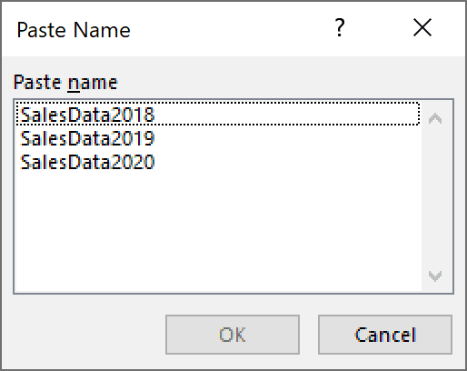
- Hit the F3 key on your keyboard. This will open the Paste Name dialog box with the list of all the names you have created
- Double-click on the name that you want to insert.
The above steps would insert the name in the formula and you can continue to work on the formula.
This is all you need to know about how to reference other sheets or workbooks and how to create an external reference in Excel.
Hope you found this tutorial useful.
You may also like the following Excel tutorials:
Источник
VBA Get Workbook Name in Excel. We can return workbook name using Workbook.Name property. Here workbook represents an object. It is part of Workbooks collection. Returns a string value representing Workbook name. We can find Active Workbook or Current Workbook name using Name property of Workbook.
Table of Contents:
- Overview
- Syntax to return Name of the Workbook VBA in Excel
- Get Name of the Active Workbook using VBA in Excel
- Macro to Get Current Workbook Name using VBA in Excel
- Instructions to Run VBA Macro Code
- Other Useful Resources
Syntax to get current Workbook name using VBA in Excel
Here is the following syntax to get the Name of the Workbook using VBA in Excel.
expression.Name
Where expression: It represents Workbook object which is part of workbooks collection.
Name: It represents property of Workbook object to get Workbook name.
Get Name of the Active Workbook using VBA in Excel
Let us see the following example macro to get current or active workbook name in using VBA in Excel. Where ‘Name’ represents the property of Workbook object. It helps to get the name of the Workbook.
'Get Active Workbook name in Excel using VBA
Sub VBA_Get_ActiveWorkbook_Name()

    'Variable declaration
    Dim sActiveWorkbookName As String

    sActiveWorkbookName = ActiveWorkbook.Name

End Sub
Output: Please find the output screenshot of the above macro code.
Macro to Get Current Workbook Name using VBA in Excel
Here is another example macro code to get current workbook name using VBA in Excel.
'Get current workbook name of the Workbook using VBA in Excel
Sub VBA_Get_CurrentWorkbook_Name()

    'Variable declaration
    Dim sCurrentWorkbookName As String

    sCurrentWorkbookName = ThisWorkbook.Name

End Sub
Output: Here is the output screenshot of the above macro code.
Instructions to Run VBA Macro Code or Procedure:
You can refer the following link for the step by step instructions to execute VBA code or procedure.
Instructions to run VBA Macro Code
Other Useful Resources:
Click on the following links of the useful resources. These helps to learn and gain more knowledge.
VBA Tutorial VBA Functions List VBA Arrays in Excel Blog
VBA Editor Keyboard Shortcut Keys List VBA Interview Questions & Answers
If you have an Excel workbook that has hundreds of worksheets, and now you want to get a list of all the worksheet names, you can refer to this article. Here we will share 3 simple methods with you.
Sometimes, you may be required to generate a list of all worksheet names in an Excel workbook. If there are only few sheets, you can just use the Method 1 to list the sheet names manually. However, in the case that the Excel workbook contains a great number of worksheets, you had better use the latter 2 methods, which are much more efficient.
Method 1: Get List Manually
- First off, open the specific Excel workbook.
- Then, double click on a sheet’s name in sheet list at the bottom.
- Next, press “Ctrl + C” to copy the name.

- Later, create a text file.
- Then, press “Ctrl + V” to paste the sheet name.

- Now, in this way, you can copy each sheet’s name to the text file one by one.


Method 2: List with Formula
- At the outset, turn to “Formulas” tab and click the “Name Manager” button.
- Next, in popup window, click “New”.

- In the subsequent dialog box, enter “ListSheets” in the “Name” field.
- Later, in the “Refers to” field, input the following formula:

=REPLACE(GET.WORKBOOK(1),1,FIND("]",GET.WORKBOOK(1)),"")

- After that, click “OK” and “Close” to save this formula.
- Next, create a new worksheet in the current workbook.
- Then, enter “1” in Cell A1 and “2” in Cell A2.
- Afterwards, select the two cells and drag them down to input 2,3,4,5, etc. in Column A.

- Later, put the following formula in Cell B1.

=INDEX(ListSheets,A1)

- At once, the first sheet name will be input in Cell B1.
- Finally, just copy the formula down until you see the “#REF!” error.


Method 3: List via Excel VBA
- For a start, trigger Excel VBA editor according to “How to Run VBA Code in Your Excel“.
- Then, put the following code into a module or project.
Sub ListSheetNamesInNewWorkbook()
    Dim objNewWorkbook As Workbook
    Dim objNewWorksheet As Worksheet

    Set objNewWorkbook = Excel.Application.Workbooks.Add
    Set objNewWorksheet = objNewWorkbook.Sheets(1)

    For i = 1 To ThisWorkbook.Sheets.Count
        objNewWorksheet.Cells(i, 1) = i
        objNewWorksheet.Cells(i, 2) = ThisWorkbook.Sheets(i).Name
    Next i

    With objNewWorksheet
         .Rows(1).Insert
         .Cells(1, 1) = "INDEX"
         .Cells(1, 1).Font.Bold = True
         .Cells(1, 2) = "NAME"
         .Cells(1, 2).Font.Bold = True
         .Columns("A:B").AutoFit
    End With
End Sub

- Later, press “F5” to run this macro right now.
- At once, a new Excel workbook will show up, in which you can see the list of worksheet names of the source Excel workbook.


Comparison
| Advantages | Disadvantages | |
| Method 1 | Easy to operate | Too troublesome if there are a lot of worksheets |
| Method 2 | Easy to operate | Demands you to type the index first |
| Method 3 | Quick and convenient | Users should beware of the external malicious macros |
| Easy even for VBA newbies |
Excel Gets Corrupted
MS Excel is known to crash from time to time, thereby damaging the current files on saving. Therefore, it’s highly recommended to get hold of an external powerful Excel repair tool, such as DataNumen Outlook Repair. It’s because that self-recovery feature in Excel is proven to fail frequently.
Author Introduction:
Shirley Zhang is a data recovery expert in DataNumen, Inc., which is the world leader in data recovery technologies, including sql fix and outlook repair software products. For more information visit www.datanumen.com
In this example, the goal is to return the name of the current workbook with a formula. This is a fairly simple problem in the latest version of Excel, which provides the TEXTAFTER function and the TEXTBEFORE function. In older versions of Excel, you can use a more complicated formula based on the MID and FIND functions. Both options rely on the CELL function to get a full path to the current workbook. Read below for details.
Get workbook path
The first step in this problem is to get the workbook path, which includes the workbook and worksheet name. This can be done with the CELL function like this:
CELL("filename",A1)
With the info_type argument set to «filename», and reference set to cell A1 in the current worksheet, the result from CELL will be a full path as a text string like this:
"C:pathtofolder[workbook.xlsx]sheetname"
Notice the workbook name is enclosed in square brackets («[name]»). The challenge then becomes how best to extract just the text between the square brackets from the path? The best way to do this depends on what Excel version you have. If you have the latest version of Excel, you should use TEXTAFTER and TEXTBEFORE functions. Otherwise, you can use the MID and FIND functions as explained below.
TEXTAFTER with TEXTBEFORE
In Excel 365, the easiest option is to use the TEXTAFTER function with the TEXTAFTER function like this:
=TEXTAFTER(TEXTBEFORE(CELL("filename",A1),"]"),"[")This is an example of nesting — the TEXTBEFORE function is nested inside of the TEXTAFTER function, and the CELL function is nested inside of TEXTBEFORE. Working from the inside out CELL returns the full path to the workbook as explained above, and the result is delivered to the TEXTBEFORE function, which extracts all text before the closing square bracket («]»):
TEXTBEFORE(CELL("filename",A1),"]")Delimiter is set to «]» in order to retrieve only text that occurs before the closing square bracket («]»). The result looks like this:
"C:pathtofolder[workbook.xlsx"This value is then delivered to the TEXTAFTER function, which is configured to return text after the opening square bracket («[«):
=TEXTAFTER("C:pathtofolder[workbook.xlsx","[")The final result from TEXTAFTER is the workbook name only:
"workbook.xlsx"Assuming a path like «C:pathtofolder[workbook.xlsx]sheetname», the final result is «workbook.xlsx».
MID + FIND function
In older versions of Excel you can get the workbook name with a more complicated formula based on the MID and FIND function:
=MID(CELL("filename",A1),FIND("[",CELL("filename",A1))+1,FIND("]", CELL("filename",A1))-FIND("[",CELL("filename",A1))-1)
This formula is annoyingly complex, mostly because older versions of Excel do not have good text parsing functions, and this means the formula needs to work in small, redundant steps. Notice the CELL function is called 4 times!
To extract the workbook name, the formula works in 5 steps:
- Get the full path and filename.
- Locate the opening square bracket («[«).
- Locate the closing square bracket («]»).
- Calculate the length of the workbook name in characters.
- Extract the text between square brackets with the MID function.
Get path and filename
To get the path and file name, we use the CELL function like this:
CELL("filename",A1) // get path and filename
The info_type argument is «filename» and reference is A1. The cell reference is arbitrary and can be any cell in the worksheet. The result is a full path like this as text:
"C:pathtofolder[workbook.xlsx]sheetname"
The path starts with the drive and includes both the workbook name and the Sheet name. Notice the workbook name appears enclosed in square brackets.
Locate opening square bracket
The location of the opening square bracket («[«) is determined like this
FIND("[",CELL("filename",A1)) // returns 19
The FIND function returns the location of «[» (19) . We then add 1 because we want to extract text starting one character after the «[«. We can now rewrite the formula like this:
=MID(CELL("filename",A1),20,FIND("]", CELL("filename",A1))-FIND("[",CELL("filename",A1))-1)
Locate closing square bracket
Next, we locate the closing square bracket «]» in the same way with the FIND function:
FIND("]", CELL("filename",A1)) // returns 33
The FIND function returns 33, from which we subtract 1, in order to extract text up through character 32.
Calculate the length of the workbook name
The final step is to extract the text between the square brackets, and this is done with the MID function. We know where we want to start (20) and where to end (32). However, while the MID function takes start_num as the starting position, there is no equivalent end_num. Instead, MID takes num_chars, the number of characters to extract. Therefore, we need to calculate num_chars by subtracting the opening bracket «[» location from closing bracket «]» location. All of the code below simply calculates the number of characters to extract:
=FIND("]", CELL("filename",A1))-FIND("[",CELL("filename",A1))-1Using our test path above, the result is 13. This is the length of the workbook name in characters.
Extract the text between the brackets
We can now rewrite the formula like this:
=MID(CELL("filename",A1),20,13)
=MID("C:pathtofolder[workbook.xlsx]sheetname",20,13)
="workbook.xlsx"
The final result is «workbook.xlsx».
I have a bit of code now that prompt the user to select a range (1 area, 1 column, several rows).
This is the code where it prompt the user to do so:
MsgBox "Select a continuous range of cells where numeric values should be appended."

Set Rng = Application.InputBox("Select a range", "Obtain Range Object", Type:=8) 'Type Values, 8 - Range object
How can I however get the Workbook name and Worksheet name from the above selection?
I need this:
- Workbook name of destination wb — this I have achieved but using cmd: ThisWorkbook (before prompting the user to do anything)
-
Worksheet name of destination ws — this would preferbly also be read from above code, where it prompt the user with «Set Rng /—/»
-
Workbook name of source wb — after reading the destination ws, I want to promt the user with a Open-dialuge to select the source Workbook, where I will promt the user to select an additional range (source range) — which will be input to 3 & 4.
-
Worksheet name of source ws — see 3
Also preferrbly I would like to have the absolute ws name ‘Sheet1’ etc. not what it is named to (e.g. Kalle Anka).
Many thanks!
EDIT: I know it in the input-dialouge show if another ws or wb is selected than from where the macro was initiated, i.e. ‘[Cognos Orders and deliveries.xlsx]Truck Orders’!$F$11:$F$18. But if I dim Set as Range — is there any way to retrive that info? If it were a String you could maybes split the String with ! and then ] to get the ws and wb seperately? How now with a Range?
EDIT2: Based on answers below, I’ve tried this with following result/problem:
Sub AppendCognosData()

Dim Rng As Range

Dim AppendWb As Workbook
Dim AppendWs As Worksheet
Dim AppendWb2 As Workbook

'Create a reference to Wb where to append data
Set AppendWb = ThisWorkbook

MsgBox "Select a continuous range of cells (in a column) where numeric values should be appended."

Set Rng = Application.InputBox("Select a range", "Obtain Range Object", Type:=8) 'Type Values, 8 - Range object

AppendWs = Rng.Parent.Name
AppendWb2 = Rng.Parent.Paranet.Name
At these 2 last rows I get Error.
- Run error nr ’91’? It says that objectvariable or With-blocvariabel
has not been designated