
Были ли сведения полезными?
(Чем больше вы сообщите нам, тем больше вероятность, что мы вам поможем.)
(Чем больше вы сообщите нам, тем больше вероятность, что мы вам поможем.)
Насколько вы удовлетворены качеством перевода?
Что повлияло на вашу оценку?
Моя проблема решена
Понятные инструкции
Понятные сведения
Без профессиональной лексики
Полезные изображения
Качество перевода
Не соответствует интерфейсу
Неверные инструкции
Слишком техническая информация
Недостаточно информации
Недостаточно изображений
Качество перевода
Добавите что-нибудь? Это необязательно
Спасибо за ваш отзыв!
×
Lesson 4: Getting Started with Excel
/en/excel2013/understanding-office-365/content/
Introduction
Excel 2013 is a spreadsheet program that allows you to store, organize, and analyze information.
While you may believe Excel is only used by certain people to process
complicated data, anyone can learn how to take advantage of the
program’s powerful features. Whether
you’re keeping a budget, organizing a training log, or creating an
invoice, Excel makes it easy to work with different types of data.
Getting to know Excel 2013
Excel 2013 is similar to Excel 2010. If you’ve previously used Excel 2010, Excel 2013 should feel familiar. If you are new to Excel or have more experience with older versions, you should first take some time to become familiar with the Excel 2013 interface.
The Excel interface
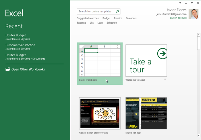
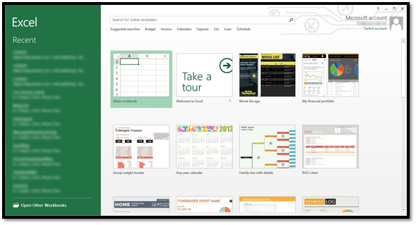
When you open Excel 2013 for the first time, the Excel Start Screen will appear. From here, you’ll be able to create a new workbook, choose a template, and access your recently edited workbooks.
- From the Excel Start Screen, locate and select Blank workbook to access the Excel interface.
 The Excel Start Screen
Click the buttons in the interactive below to become familiar with the Excel 2013 interface.
Working with the Excel environment
If you’ve previously used Excel 2010 or 2007, Excel 2013 will feel familiar. It continues to use features like the Ribbon and Quick Access toolbar, where you will find commands to perform common tasks in Excel, as well as Backstage view.
The Ribbon
Excel 2013 uses a tabbed Ribbon system instead of traditional menus. The Ribbon contains multiple tabs, each with several groups of commands. You will use these tabs to perform the most common tasks in Excel.
Click the arrows in the slideshow below to learn more about the different commands available within each tab on the Ribbon.

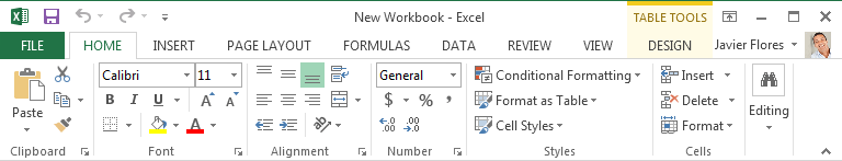
The Home tab gives you access to some of the most commonly used commands for working with data in Excel 2013, including copying and pasting, formatting, and number styles. The Home tab is selected by default whenever you open Excel.
-
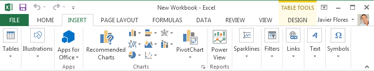
The Insert tab allows you to insert charts, tables, sparklines, filters, and more, which can help you visualize and communicate your workbook data graphically.
-
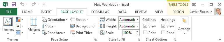
The Page Layout tab allows you to change the print formatting of your workbook, including margin width, page orientation, and themes. These commands will be especially helpful when preparing to print a workbook.
-
The Formulas tab gives you access to the most commonly used functions and formulas in Excel. These commands will help you calculate and analyze numerical data, such as averages and percentages.
-
The Data tab makes it easy to sort and filter information in your workbook, which can be especially helpful if your project contains a large amount of data.
-
You can use the Review tab to access Excel’s powerful editing features, including comments and track changes. These features make it easy to share and collaborate on workbooks.
-
The View tab allows you to switch between different views for your workbook and freeze panes for easy viewing. These commands will also be helpful when preparing to print a workbook.
-
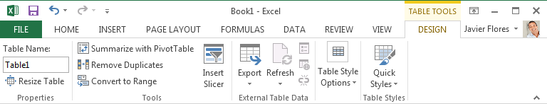
Contextual tabs will appear on the Ribbon when working with certain items, like tables and pictures. These tabs contain special command groups that can help you format these items as needed.
Certain programs, such as Adobe Acrobat Reader, may install additional tabs to the Ribbon. These tabs are called add-ins.
To minimize and maximize the Ribbon:
The Ribbon is designed to respond to your current task, but you can choose to minimize it if you find that it takes up too much screen space.
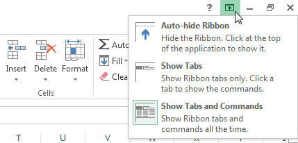
- Click the Ribbon Display Options arrow in the upper-right corner of the Ribbon.
 Ribbon Display options
 - Select the desired minimizing option from the drop-down menu:
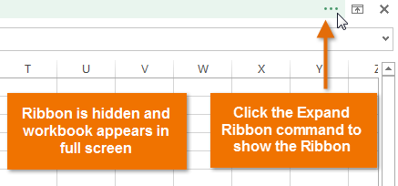
- Auto-hide Ribbon: Auto-hide displays your workbook in full-screen mode and completely hides the Ribbon. To show the Ribbon, click the Expand Ribbon command at the top of screen.
 Auto-hiding the Ribbon
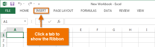
 - Show Tabs: This option hides all command groups when they’re not in use, but tabs will remain visible. To show the Ribbon, simply click a tab.
 Showing only Ribbon tabs
 - Show Tabs and Commands: This option maximizes the Ribbon. All of the tabs and commands will be visible. This option is selected by default when you open Excel for the first time.
- Auto-hide Ribbon: Auto-hide displays your workbook in full-screen mode and completely hides the Ribbon. To show the Ribbon, click the Expand Ribbon command at the top of screen.
To learn how to add custom tabs and commands to the Ribbon, review our Extra on Customizing the Ribbon.
To learn how to use the Ribbon with touch-screen devices, review our Extra on Enabling Touch Mode.
The Quick Access toolbar
Located just above the Ribbon, the Quick Access toolbar lets you access common commands no matter which tab is selected. By default, it includes the Save, Undo, and Repeat commands. You can add other commands depending on your preference.
To add commands to the Quick Access toolbar:
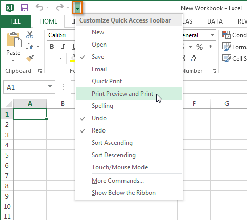
- Click the drop-down arrow to the right of the Quick Access toolbar.
- Select the command you want to add from the drop-down menu. To choose from more commands, select More Commands.
 Adding a command to the Quick Access toolbar
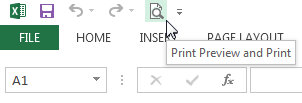
 - The command will be added to the Quick Access toolbar.
 The added command
Backstage view
Backstage view gives you various options for saving, opening a file, printing, and sharing your workbooks.
To access Backstage view:
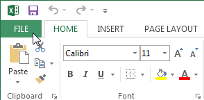
- Click the File tab on the Ribbon. Backstage view will appear.
 Clicking the File tab
Click the buttons in the interactive below to learn more about using Backstage view.
Worksheet views
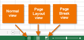
Excel 2013 has a variety of viewing options that change how your workbook is displayed. You can choose to view any workbook in Normal view, Page Layout view, or Page Break view. These views can be useful for various tasks, especially if you’re planning to print the spreadsheet.
- To change worksheet views, locate and select the desired worksheet view command in the bottom-right corner of the Excel window.
 Worksheet view options
Click the arrows in the slideshow below to review the different worksheet view options.

Normal view: This is the default view for all worksheets in Excel.
-
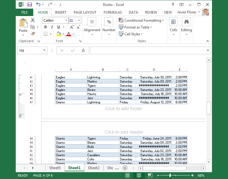
Page Layout view: This view can help you visualize how your worksheet will appear when printed. You can also add headers and footers from this view.
-
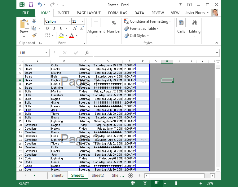
Page Break view: This view makes it easy to change the location of page breaks in your workbook, which is especially helpful when printing a lot of data from Excel.
Challenge!
- Open Excel 2013.
- Click through all of the tabs, and review the commands on the Ribbon.
- Try minimizing and maximizing the Ribbon.
- Add a command to the Quick Access toolbar.
- Navigate to Backstage view, and open your Account settings.
- Try switching worksheet views.
- Close Excel (you do not have to save the workbook).
/en/excel2013/creating-and-opening-workbooks/content/
Microsoft Excel is a spreadsheet program that comes packaged with the Microsoft Office family of software products. Just like the other programs by Microsoft, Excel can be used for a wide variety of purposes such as creating an address book, grocery lists, tracking expenses, creating invoices and bills, accounting, balancing checkbooks and other financial accounts, as well as any other purpose that requires a spreadsheet or table.
About Excel 2013
Excel is much more than a basic spreadsheet program. It gives you the complex tools and features you need to design professional spreadsheets, but all with just a few clicks of the mouse.
The good news is that Excel makes everything easy. By learning how to navigate the program, and where to find each feature, operating Excel can become a breeze!
You can use Excel to:
-
Organize, sort, and record data.
-
Enter in text and mathematical data.
-
Keep statistics.
-
Keep records.
-
Create mathematical equations and functions to accurately keep records, statistics, and data.
-
And much more!
Downloading Excel 2013
With the launch of Office 2013, Microsoft made changes in how they sell their most popular software package. Of course, you can download a free trial by simply going to the Microsoft Office page, picking out what version you want to try, then downloading the software. You don’t need a credit card to try the software.
If you want to purchase the software, Microsoft now gives you two choices. As always, you can buy the software — either online or from most office supply or computer stores. The prices to buy the software vary depending on what version you wish to purchase. There are three versions: Home and Student, Home and Business, and Professional. As with other versions of Office, it’s a one time charge and the software is yours to use as long as you wish.
However, with Office 2013 also comes Office 365, which is another method that you can use to buy the Office suite of software. With Office 365, you subscribe to the software instead of just purchasing it like you’ve done in the past. You can pay for your subscription by the month or year on the Microsoft Office website. The price of your subscription will be determined by the version that you want: Home, Small Business, or Mid-size Business.
Once you purchase a subscription, you’ll be able to download Office 2013 on your computer just as you would if you had bought the software in a store. As part of Office 365, you’ll also be given multiple licenses, which will give you the ability to install the software on other computers, as well. This is a perk that doesn’t come with buying the software in a store. For the Home version, you get up to five licenses (five devices). The Small Business version comes with licenses for up to 25 users. The Midsize Business provides for up to 300 users. There’s also an Enterprise version for larger companies that offers unlimited users.
Once you subscribe to Office 365, you’ll never have to worry about purchasing a new version of Office ever again. When a new version comes out, your software will be updated for you.
What’s New in Excel 2013
Excel 2013 is arguably the best version yet. It contains the same great features you loved in past versions, which have been fine tuned and improved for better usability. In addition, it contains some great new features that make Excel even more useful and functional than ever before.
Here are the improvements:
-
The new Start Screen makes getting started in Excel easier than ever. You can start a blank spreadsheet, or open a template – and get busy!
-
The new Quick Analysis tool makes it easy to convert data into a chart or table. All it takes is two steps (sometimes even less).
-
Flash Fill finishes your work for you in 2013. When Excel detects a pattern in your data, it enters the rest of the data for you.
-
Don’t know what type of chart to use? Chart recommendations now shows you the best chart for your data.
-
Improved slicers can now filter data in tables and query tables.
-
Each workbook now has its own window.
-
New functions
-
Save and share files online – for free!
-
Embed your worksheet data in a web page
-
The new Design and Format tabs make it easier to format charts and tables.
-
View animation in charts
-
And more!
Getting Started In Microsoft Excel
You open Microsoft Excel by clicking on the icon on your desktop (if you have one there) or in the program bar. The icon for Microsoft Excel 2013 looks like this:

When you click on the icon, Excel 2013 will open, and you’ll see the Start Screen. This is new to 2013.
The Start Screen looks like this:
On the left, you’ll see the dark green column that contains your recently opened files. You can click on any of these to open them. To the right, you’ll see templates you can use to start a new Excel workbook. You can also choose to just open a workbook, as we’ve selected above.
Let’s open a blank spreadsheet.
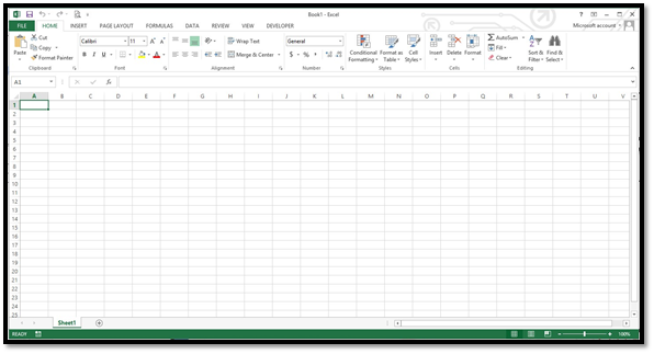
This is a new workbook for which the default name is Book1. You can see the name in the Title bar.

For each additional new workbook that you open, the name increases by one digit: Book2, Book3, etc. If you start MS Excel by clicking on an already existing workbook on your computer, it will open automatically and your workbook will be displayed in the MS Excel window.
Touring the Excel 2013 Interface
Let’s take a look at the blank workbook again. This time, however, we’ve labeled the different parts of the interface that you’ll use in Excel 2013.
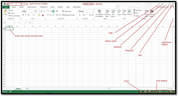
Take a few minutes to look at the features that we’ve labeled for you. It’s not important that you know how to use these things right now. For now, just take a second to familiarize yourself with where everything is located. The items labeled above help to make using Excel 2013 easier, but they’re not the bread and butter.
If you look below the Quick Access Toolbar (as labeled above), you’ll see the Ribbon. The Ribbon was first introduced in Office 2007.

The ribbon is divided into tabs. These tabs are also menus. The tabs are Home, Insert, Page Layout, Formulas, Data, Review, View, and Developer.
Below each tab are commands (or tools) you can use. The commands (or tools) located beneath each tab relate to the tab. For example, under the Page Layout tab, you would find tools to create a page layout.
That said, the tools under each tab are broken down into groups so that you can easily find what you need. In the snapshot above, we’re looking at Home. The groups within the Home tab are Clipboard, Font, Alignment, Number, Styles, Cells, and Editing. Below is a snapshot of the Alignment group.
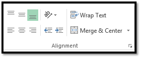
In the Alignment group are all the tools that are related to alignment.
If you look to the right of the word «Alignment,» you’ll see an arrow in the lower right corner. If you click this, it will take you to the Alignment options dialog box. You can click this arrow in any group to open the options for that group.
Working with Excel 2013 on a Tablet
If you’re using Excel on a tablet, you can adjust the spacing between buttons on the ribbon to make it easier to use. You do this by activating Touch mode.
To do this, click or touch the Quick Access Toolbar button:
Select Touch/Mouse Mode.
You can now see the button in the Quick Access Toolbar, as shown below:
Now, touch or click the button and choose Touch.
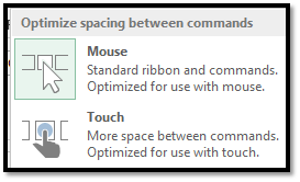
There is now more space between commands on the Ribbon.
Learning how to navigate around Excel is critical to being able to successfully use the program. In this section, we’re going to focus on the major elements of Excel 2013 and take a few minutes to become familiar with their purpose.
If you have access to Excel 2013, you should open a blank spreadsheet at this time.
Understanding the Basic Elements of an Excel Spreadsheet
Before going any further in this section, it’s important to understand the elements of a spreadsheet, in Excel, or any spreadsheet that you may use.
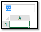
A spreadsheet is made up of individual cells. One cell is simply a block on your screen. In the snapshot below, you can see a cell that’s highlighted:
The cell above is highlighted because it’s an active cell. In other words, we clicked on it with our mouse to make it active so we can enter data into it.
Now, all the cells in a worksheet are organized into columns and rows. In Excel, rows are represented by numbers. Columns are represented by letters.
Below is a snapshot of row 5, followed by a snapshot of column C.

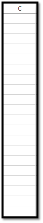
Rows are horizontal. Columns are vertical.
Since rows and columns are labeled with numbers and letters respectively, you can also locate the exact coordinates of a cell.
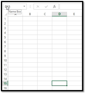
For example, instead of your boss coming to you and telling you the number for March’s expenses for employee Susie Smith are wrong, he can simply say, recheck the number in D15. This would tell you to go to column D, row 15.
Then, instead of scrolling through your worksheet, simply go to the Name box above Column A (pictured below). In the snapshot below, you’ll see A1 highlighted in blue. This is the Name box.
Enter the coordinates for the cell. We’re going to enter D15, then hit Enter.
As you can see below, Excel took us to the exact cell and highlighted it for us.
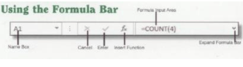
The Formula Bar
The formula bar is the magical ingredient of the soup, so to speak. It is what makes Excel easier to use than doing spreadsheets by hand, or using other programs where you’re left to do the math by yourself.
In this section, you’ll learn how to enter formulas and equations into MS Excel 2013. The formulas and equations that you enter will be entered in and displayed in the Formula Bar. It is located to the right of the Name Box.

The Formula Bar has the fx to the left of it.
On the left side of the Formula Bar are the Formula Bar buttons. The Insert Function button is fx. When you start making or editing a cell entry, X is Cancel and the check mark is Enter.
The white area (or bar) to the right of the buttons is the Cell Contents area. The Formula Bar always shows you the contents of a cell, even if it doesn’t appear in the cell. In other words, it shows equations in the cell even if the cell only displays the answer to the equation. It will show contents of cells that appear to be blank in the spreadsheet as well. If the Cell Contents area is blank, you know the cell is empty.
The Backstage Area
The Backstage area is located under the green File tab at the upper left hand corner of the Excel window. If you click on it, this is what you see:
Using the Backstage area, you can open an existing spreadsheet, create new spreadsheet (either blank or template), save workbooks and spreadsheets, share workbooks and spreadsheets, print, close, and set options for the Excel program.
Click the left facing arrow at the top left of the Backstage area to go back to your spreadsheet.
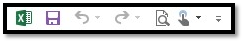
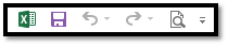
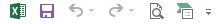
The Quick Access Toolbar
The Quick Access Toolbar is located at the top left of the Excel window. It looks like this:
You can use the Quick Access toolbar to add shortcuts to tools that you use frequently, rather than having to click tabs and find the tools in a group.
By default, our Quick Access toolbar displays these shortcuts:
 Save
Save
 Undo
Undo
 Redo
Redo
 Print Preview/Print
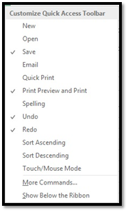
You can customize the Quick Access toolbar and add shortcuts so the tools you need appear there for easy access.
Click the drop-down menu to the right of the toolbar. It looks like this: 
Now, click on the shortcuts you want to add to the toolbar from the list. When you click on a shortcut, it will put a check mark beside it, letting you know it appears on the toolbar.
If you want to add a shortcut for a tool, but you don’t see it on the Customize Quick Access Toolbar list, you can still add it to your toolbar. You do this by adding Ribbon commands.
Simply go to the Ribbon and find the tool that you want to add. Right click on the tool (or tab and hold if you’re using a touchscreen device).
In this example, we’re going to add SmartArt under the Insert tab.
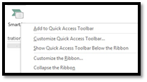
Select Add to Quick Access Toolbar.
As you can see, it’s now added:
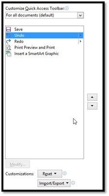
If you want to move a command button in the toolbar to a different location or group it with other buttons on the toolbar, select the Customize Quick Access Toolbar downward arrow (on the Quick Access toolbar), then select More Commands.
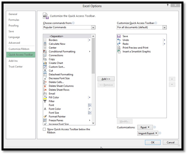
On the right side, you can see everything that’s added to the Quick Access toolbar. They are listed in the order they appear on the toolbar.
If you want to change its location, click on it to select it, then use the arrows to the right to move it up or down.
If you want to group buttons on the Quick Access toolbar, you can add vertical separators. To do this, select <Separator> from the list on the left:
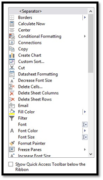
Then click the Add button twice.
To add shortcuts listed in the left column, click the shortcut to select it, then click the Add button.
To remove shortcuts from the Quick Access toolbar, select the shortcut in the right column, then click the Remove button.
Moving Around Worksheets
Being able to navigate through a worksheet will make using Excel a lot easier. However, before we discuss that, let’s quickly review three things you have to know about the worksheet area. Remember, the worksheet area contains cells, rows, and columns.
-
The cell cursor is the dark green border that appears around a cell. It means a cell is active.
-
The location of the cell, or address, appears in the Name box.
-
The cell’s row number and column letter are shaded. Look at the snapshot below. Note that the row number 1 is shaded differently than the rows after. Note that the column A is shaded differently than the other columns.
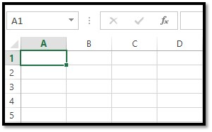
This is because cell A1 is active, as confirmed by the Name box and the green border around the cell.
Now, since the Excel worksheet contains so many cells, rows, and columns, not all of your cells are going to be displayed at once on the screen. For that reason, there are several ways that you can use your mouse cursor to move through and navigate your worksheet.
Of course, if the cell is displayed, you can simply click on it to make it active. If you’re using a touchscreen, just tap it.
You can also type the coordinates in the Name box and be taken to the cell.
Press F5 to open the Go To dialog box.
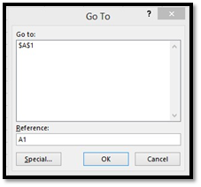
All you have to do is type the address of the cell in the Reference box (pictured above).
You can also use cursor keys to move to the desired cell. The cursor keys are displayed in the table below:
|
Keystroke |
Action |
|
Moves cell to the right |
|
? on the keyboard or Shift+Tab |
Moves cell to the left |
|
Up arrow on the keyboard |
Moves one cell up |
|
Down arrow on the keyboard |
Moves one cell down |
|
Home |
Moves cursor to cell in Column A of the current row |
|
Ctrl+Home |
Moves cursor to the first cell — A1 |
|
Ctrl+End or End, Home |
Moves the cursor to the cell that’s at the intersection of the last column with data and the last row that has data in it |
|
Page Up |
Moves the cursor to cell that’s one full screen up in the same column |
|
Page down |
One full screen down (in the same column) |
|
Ctrl+? or End, ? |
Moves the cursor to the first occupied cell that’s to the right that’s has a blank cell before it or after it. If there isn’t an occupied cell, it goes to the end of the row |
|
Ctrl+? or End, ? |
Same as above, except first occupied cell to the left. |
|
Ctrl+ Up arrow, or End, Up Arrow |
Moves the cursor to the first occupied column above that has a blank cell before it or after it. |
|
Ctrl+Down arrow, or End, Down arrow |
Same as above, except for first occupied cell below. |
|
Ctrl+Page Down |
The cursor moves to the next worksheet of the workbook |
|
Ctrl+Page Up |
Moves to the previous sheet of the workbook |
Using the Touch Keyboard
If you’re using Excel on a tablet or other touch-enabled device, you can also use the on-screen touch keyboard. Instead of entering characters (letters, numbers, and spaces) by pecking away on your keyboard, you’ll simply touch your finger or stylus pen to the keyboard on the screen.
Make sure you enable Touch mode before starting to use Excel from a tablet or touch device.
To use the on-screen keyboard, simply tap in the spreadsheet area to see the cursor – and the keyboard.
The Status Bar
The Status Bar appears at the bottom left of your Excel window. It contains the following information about your spreadsheet:
-
Mode Indicator shows the state of your Excel program, such as Ready, Edit, etc. It will also tell you if any special keys are in use, such as Caps Lock.
-
AutoCalculate Indicator shows the average and sum of all the numerical entries for the current cell selected, as well as the count of every cell in the selection.
-
Layout Selector allows you to select between three different layouts for the worksheet area: Normal (default), Page Layout View, and Page Break View. We’ll discuss views later in the section.
-
The Zoom Slider lets you zoom in and out of areas on a worksheet to see more/less cells.
The Status Bar is pictured below:

17788

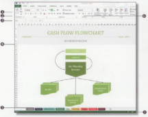
Excel 2013: Краткое руководство по началу работы + ВИДЕО
Интерфейс Microsoft Excel 2013 изменился по сравнению с предыдущими версиями, и чтобы помочь вам быстрее освоиться с ним, мы представляем вашему вниманию это руководство.
Используйте контекстные меню: Часто удобно использовать контекстные меню, которые можно вызвать, щелкнув правой кнопкой мыши лист, диаграмму или сводную таблицу. В них доступны команды, актуальные в текущем контексте.
Используйте подсказки к клавишам: Если вы предпочитаете использовать клавиатуру, нажмите клавишу ALT, чтобы увидеть клавиши, с помощью которых можно вызывать команды на ленте. Кстати, сочетания клавиш, использовавшиеся ранее, по-прежнему работают.
Обращайте внимание на визуальные подсказки: Используйте управляющие кнопки, появляющиеся на листе, и отслеживайте изменения с помощью анимации.
- Добавляйте команды на панель быстрого доступа: Часто используемые команды и кнопки останутся видны, даже если вы скроете ленту.
- Используйте команды на ленте: Каждая вкладка ленты разбита на группы связанных команд.
- Отображайте или скрывайте ленту: Чтобы скрыть или показать ленту, щелкните значок Параметры отображения ленты или нажмите клавиши CTRL+F1.
- Открывайте диалоговые окна: Чтобы просмотреть дополнительные параметры группы, нажмите кнопку вызова диалогового окна.
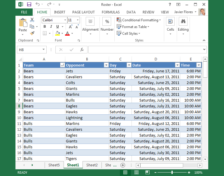
- Изменяйте режим просмотра: Используйте режим, в котором удобнее всего работать. Можно выбрать режим Обычный, Разметка страницы или Страничный.
- Изменяйте масштаб: Чтобы изменить масштаб, перетащите этот ползунок.
- Создавайте листы: Начав с одного листа, можно добавлять другие по мере необходимости.
- Управляйте файлами: Открывайте, сохраняйте, печатайте файлы и делитесь ими. В этом представлении также можно изменять параметры программы и учетных записей.

Используйте контекстные меню
Начало работы с Excel 2013
Если вы уже работали с приложением Excel 2007 или 2010 и знакомы с лентой, то захотите узнать, что изменилось в Excel 2013. Если же вы до сих пор использовали Excel 2003, наверняка вам потребуется найти на ленте команды и кнопки, которые были доступны в Excel 2003.
Начало работы с Excel 2013
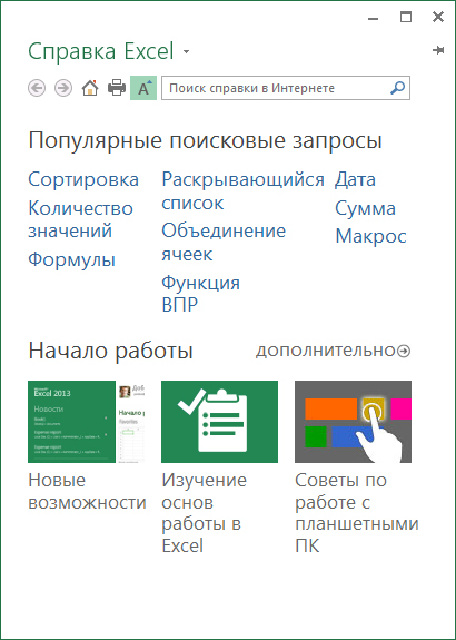
Мы предлагаем множество бесплатных ресурсов по обучению работе с Excel 2013, в том числе в Интернете. Чтобы открыть справку Excel, просто щелкните вопросительный знак в правом верхнем углу над лентой.
Новые возможности ленты
Если вы уже пользовались лентой в одной из предыдущих версий Excel, то заметите ряд изменений.

Новые возможности ленты
На вкладке Вставка появились новые кнопки для создания диаграмм и сводных таблиц. Также теперь доступна новая группа Фильтры с кнопками для создания срезов и временных шкал.

Также теперь доступна новая группа Фильтры с кнопками
При работе с определенными объектами, например диаграммами и сводными таблицами, появляются дополнительные вкладки. Их мы также изменили, чтобы сделать поиск команд еще проще.
Действия, которые вам могут потребоваться
Из приведенной ниже таблицы вы узнаете, где найти некоторые наиболее часто используемые инструменты и команды в Excel 2013.
| Действия | Вкладка | Группы |
|---|---|---|
| Создание, открытие, сохранение, печать, экспорт файлов, предоставление общего доступа к ним и изменение параметров | Файл | Представление Backstage (выберите команду в области слева) |
| Форматирование, вставка, удаление, изменение и поиск данных в ячейках, столбцах и строках | Главная | Группы Число, Стили, Ячейки и Редактирование |
| Создание таблиц, диаграмм, спарклайнов, отчетов, срезов и гиперссылок | Вставка | Группы Таблицы, Диаграммы, Спарклайны, Фильтры и Ссылки |
| Настройка полей и разрывов страниц, областей печати и параметров листов/td> | Разметка страницы | Группы Параметры страницы, Вписать и Параметры листа |
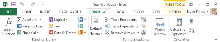
| Поиск функций, определение имен и устранение неполадок с формулами | Формулы | Группы Библиотека функций, Определенные имена и Зависимости формул |
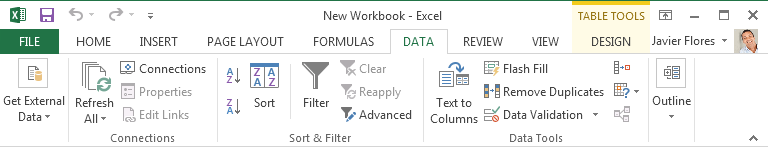
| Импорт данных, подключение к ним, сортировка, фильтрация и проверка данных, мгновенное заполнение значений и анализ «что если» | Данные | Группы Получение внешних данных, Подключения, Сортировка и фильтр и Работа с данными |
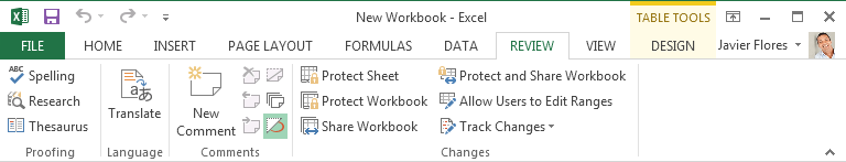
| Проверка орфографии, рецензирование и внесение исправлений, защита листа или книги | Рецензирование | Группы Правописание, Примечания и Изменения |
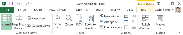
| Изменение режима просмотра книги, упорядочение окон, закрепление областей и запись макросов | Вид | Группы Режимы просмотра книги, Окно и Макросы |
Применение функций без использования ленты
В Excel 2013 некоторые часто использовавшиеся, но труднодоступные команды и кнопки теперь находятся под рукой. При выделении данных на листе появляется кнопка Быстрый анализ. С ее помощью можно быстро получить доступ ко множеству полезных функций, о существовании которых вы, возможно, не догадывались, и предварительно просмотреть результат их применения.

Применение функций без использования ленты
При вводе данных Excel заполняет значения автоматически, если определяет, что они соответствуют некоторому шаблону. При этом появляется кнопка Параметры мгновенного заполнения, предоставляющая доступ к дополнительным командам.

При вводе данных Excel заполняет значения автоматически
Улучшенный доступ к функциям диаграмм
Чтобы быстро создать диаграмму, можно выбрать один из рекомендованных вариантов, однако при этом все же потребуется настроить ее стиль и заполнить собственными данными.
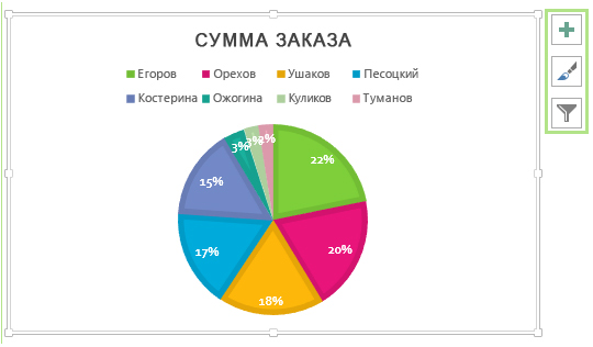
Улучшенный доступ к функциям диаграмм
В Excel 2013 соответствующие элементы находятся непосредственно рядом сдиаграммой. Чтобы настроить ее, просто нажмите кнопку Элементы диаграммы, Стили диаграмм или Фильтры диаграммы.
Совместная работа с пользователями предыдущих версий Excel
Предоставляя общий доступ к файлам или обмениваясь ими с людьми, которые работают с одной из предыдущих версий Excel, учитывайте указанные ниже моменты.
| Действие в Excel 2013 | Что происходит | Что нужно сделать |
|---|---|---|
| Вы открываете книгу, созданную в Excel 97–2003 | Книга открывается в режиме совместимости и остается в формате Excel 97–2003 (XLS). Если вы использовали новые возможности, которые не поддерживаются в более ранних версиях Excel, при сохранении книги будет выведено предупреждение о проблемах с совместимостью. | Если вы совместно работаете над книгой с пользователями предыдущих версий Excel, продолжайте использовать режим совместимости. В противном случае преобразуйте ее в формат Excel 2007–2013 (XLSX), чтобы использовать новые возможности Excel 2013 (выберите пункты Файл → Сведения → Преобразовать). |
| Вы сохраняете книгу в формате Excel 2013 | Книга сохраняется в формате Excel 2007–2013 (XLSX), что позволяет использовать все новые возможности Excel 2013. | Если вы планируете предоставлять общий доступ к книге пользователям более ранних версий Excel, проверьте ее на наличие проблем с совместимостью (выберите пункты Файл → Сведения → Поиск проблем). Прежде чем предоставлять общий доступ к книге, можно просмотреть проблемы и устранить их. |
| Вы сохраняете книгу в формате Excel 97–2003 | Excel автоматически проверяет файл на наличие проблем с совместимостью и показывает, какие новые возможности Excel 2013, не поддерживаемые в прежних версиях, вы использовали. | Оцените проблемы и устраните их, прежде чем предоставлять общий доступ к книге. |
Доступ к дополнительным возможностям
Чтобы изредка записать макрос, можно использовать кнопку Макросы на вкладке Вид. Но если нужно регулярно создавать или изменять макросы и формы либо использовать решения XML и VBA, рекомендуется добавить на ленту вкладку Разработчик. Это можно сделать в диалоговом окне Параметры Excel на вкладке Настройка ленты (выберите пункты Файл → Параметры → Настроить ленту).
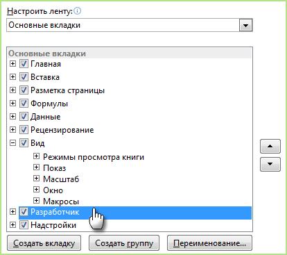
Доступ к дополнительным возможностям
Вкладка Разработчик появится на ленте справа от вкладки Вид.
Включение надстроек Excel
Excel 2013 включает ряд надстроек, которые расширяют возможности анализа данных. Некоторые из них, например «Пакет анализа» или «Поиск решения», использовались и в предыдущих версиях Excel. Чтобы добавить надстройку на ленту, нужно включить ее. Для этого в диалоговом окне Параметры Excel на вкладке Надстройки (Файл → Параметры → Надстройки) выберите в поле Управление соответствующий пункт и нажмите кнопку Перейти.
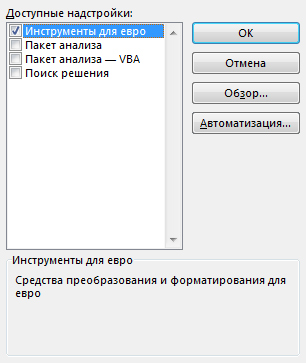
Excel 2013 включает ряд надстроек, которые расширяют возможности анализа данных
В версии Office профессиональный плюс доступны некоторые новые надстройки, такие как Inquire, PowerPivot for Excel 2013 и Power View. Для надстройки Power View даже отображается отдельная кнопка на вкладке Вставка. При первом нажатии этой кнопки надстройка включается.
Excel 2013 — Getting Started
The Excel Window
- 1. Quick Access Toolbar — contains shortcuts for the most commonly used tools.
- Backstage View – contains tools to work with workbook files and manage Excel settings.
- Ribbon – contains groups of tools for use with the Excel 2013.
- Worksheet Area – displays the current worksheet.
- Sheet Tabs – displays tabs for the sheets in the current workbook.
- Tab Bar – contains tabs that display tools and commands in the ribbon.
- Status Bar – contains worksheet information and shortcuts.
Customizing the Ribbon
To optimize Excel for the tools and features you use most, you can customize the toolbars and ribbon.
∙ To customize the Quick Access Toolbar, click the Customize Quick Access Toolbar button in the top right corner of the toolbar.
Check or uncheck commands from the resulting menu to add or remove shortcuts.
∙ To hide the Ribbon, Click the Customize the Ribbon button in the top right corner of the screen. Click Auto-Hide Ribbon to hide the entire ribbon. Click Show Tabs to only show the ribbon’s tab headings. Click Show Tabs and Commands to restore the ribbon again once you have hidden it.
Using the Backstage View
The Backstage view replaces and expands on the File menu. The Backstage view allows you to quickly manage Excel settings as, functions, and options. To access the Backstage view, click on the File tab on the Tab Bar. Make selections in the Left pane. Click the Back button to exit.
Creating a New Workbook
1. Click on the File tab
2. Select New in the left pane. From here, you can do one of the following from the Available Templates pane:
∙ To select a blank workbook, select Blank workbook.
∙ To use a default template, scroll through listed templates.
∙ To look through commonly searched template, click the options in the Suggested searches spaces.
∙ To search the web for a template, click in the Search for online templates bar. Enter your search query and click the Search button.
Opening a Workbook
- Click on the File tab.
- Select Open in the left pane.
- Select the location where your file is stored from Recent Workbooks or your Computer.
- Click the Browse button. Select the workbook file
- Click Open.
Saving a Workbook
1. Click on the File tab.
2. Do one of the following:
∙ To save the document as an Excel 2013 file (.xls), Save from the left pane.
∙ To save the document as another file format, select Save As in the left pane. Select the location you would like to save the file to and click Browse. Click the arrow on the Save as type box and select a format from the resulting menu.
3. Select the location where you want to save the workbook.
4. Enter a file name in the File name box.
5. Click the Save button.
Worksheets
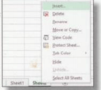
Inserting a Worksheet
∙ To insert a new worksheet at the end of existing worksheets, click the Insert Worksheet button on the right side of the row of worksheet tabs.
∙ To insert a new worksheet before an existing worksheet, select the worksheet and click on the Home tab. Click the arrow on the Insert Cells button in the Cells group and select Insert Sheet from the resulting menu.
Renaming a Worksheet
- Right click the tab for the worksheet you want to
- rename.
- Select Rename from the short cut menu.
- Enter a name for the worksheet and press the Enter key.
Moving or copying a Worksheet.
1. Right click the tab for the worksheet you want to move or copy.
2. Select Move or Copy from the shortcut menu.
Select the worksheet you want to move or copy.
3. Do one of the following:
∙ To copy the selected worksheet, check the
Create a copy box.
∙ To move the selected worksheet, clear the
Create a copy box.
4. Click the OK button.
Deleting a Worksheet
1. Select the worksheet you want to delete.
2. Click on the Home tab.
3. 3. Click the arrow on the Delete
button in the Cells group.
4. Select Delete Sheet from the resulting menu.
Rows & Columns
Inserting a Rows or Column
1. Select the row heading below or the column hearing to the right of where you want to insert the row or column. (To insert multiple rows or columns, elect the same number of columns or rows that you want to insert.)
2. Click on the Home tab.
3. Click the arrow on the Insert Cells button in the Cells group.
4. Select Insert Sheet Rows or Insert Sheet Columns from the resulting menu.
Cells
Selecting Cells
∙ To select a single cell, click on the cell.
∙ To select a range of cells, click on the first cell in the range, hold the Shift key, and click on the last cell in the range, or click and drag the mouse pointer over the range of cells.
∙ To select multiple
nonadjacent cells, hold the Ctrl key and click on each cell you want to select.
∙ To select all the cells in a worksheet, click the Select
All button in the upper left corner of the worksheet.
Inserting Cells
- Select the cell or range of cells where you want to insert the new blank cells.
- Click on the Home tab.
- Click the arrow on the Insert Cells button in the Cells group.
- Select Insert Cells from the resulting menu.
- Select how you want to shift the cells and click the OK button.
Formatting Cells
- Select the cells you want to change the formatting for.
- Click the Home tab.
- Click the Format button in the Cells group.
- Select Format Cells from the resulting menu.
- Make formatting selections in the Format Cells dialog box. 6. Click the OK button when you are finished.
Merging Cells
Merge cells to spread the contents of one cell over several cells.
- Copy the data into the upper left cell of the range.
- Select the cells you want to merge.
- Click on the Home tab. 4. Click the arrow on the Merge & Center button in the
Alignment group and do one of the following:
∙ To merge the cells and center the text, select
Merge & Center from the resulting menu.
∙ To merge without centering, select Merge
Across or Merge Cells
from the resulting menu.
Data
Enter data into cells by double-clicking until the flashing text cursor appears. You can also use the Copy and Paste functions to input large amounts of data.
Using Auto Fill
Excel can automatically fill in a series of numbers, dates, or other sequential items.
- Select the first cell in the range you want to fill.
- Enter the starting value
- Enter a value in the next cell to establish a pattern.
- Select the cell or cells that contain the starting values.
- Drag the fill handle over the range you want to fill. To fill in a numerically increasing order, drag down or to the right.
Clearing Cell Format or Contents
- Select the cells you want to clear of formatting or contents.
- Click on the Home tab.
- Click the Clear button in the Editing group.
- Select one of the following from the resulting menu:
∙ To clear everything in the cells, select Clear All.
∙ To clear the formatting of the cell, select Clear
Formats.
∙ To clear the contents of the cell, select Clear Contents.
Formulas
Creating a Formula
- Select the cell that will contain the formula.
- Enter an equal sign (=) in the Formula Input Area.
- Enter the formula in the Formula Input Area using the following guidelines:
∙ The four types of operators are Add (+),
Subtract (-), Multiply (*),
and Divide (/).
∙ Reference cells by their cell number (i.e. Al, B8).
∙ Enter parentheses around calculations that are to be performed first.
Inserting a Function
1. Select the cell that will contain the formula.
2. Click the Insert Function button on the Formula Bar.
(You can also click on the Formulas tab and click the Insert Function button in the Function Library group.)
3. Do one of the following:
∙ To search for a function, enter a description of the function in the Search for a function box and click the Go button.
∙ To select a category, click the arrow on the Or select a category box and select a category from the resulting menu.
4. Select the function you want to use and click the OK button.
5. Enter the arguments for the function in the Function
Arguments dialog box.
(Arguments are the values that a function uses to perform a calculation or operation.)
6. Click the OK button when you are finished.
Using the Sum Button
- Click a cell below the column or to the right of the row of numbers you want to evaluate.
- Click on the Home tab.
- Click the arrow on the Sum button in the Editing group.
- 4. Select a function from the resulting menu.
- Do one of the following:
∙ To use the highlighted cells, press the Enter key.
∙ To change the highlighted cells, select other cells and press the Enter key.
Understanding Cell References
∙ A reference identifies a cell or range of cells on a worksheet and tells the formula where to look for data.
∙ A relative cell reference is relative to the position of the formula. If the position of the cell that contains the formula changes, the reference is changed.
∙ An absolute cell reference always refers to a specific location,
regardless of where the formula is located. To indicate an absolute reference, place a dollar sign ($) before the letter and number of the cell reference, such as $B$2.
Illustrations
Inserting an Illustration
1. Click on the workbook where you want to place the illustration. 2. Click on the Insert tab.
3. In the Illustrations group, do one of the following:
∙ To insert a picture from a file, click the Picture
button. Locate and select
the graphic file you want
to insert and click the
Insert button.
∙ To insert a graphic or clip art from the internet, click
the Online Pictures
button. Enter a keyword
for the clip are you want to
insert in the Search for box
in the Clip Art task pane.
Click the Enter button.
Click on the graphic you
want to insert in the
resulting pane.
∙ To insert a shape, click the Shapes button and select a shape from the
resulting menu. Click and drag in the worksheet to create the shape.
∙ To insert a SmartArt graphic, Click the Smart Art button. Select a category in the left pane and select the SmartArt graphic you want to insert. Click the OK button.
Using Quick Analysis
The Quick Analysis feature provides instant links to powerful tools to analyze your data through a chart, formula, sparkline, or other graphical representation.
1. Click and drag to select the table you wish to work with.
2. When the Quick Analysis button arrears, click it to open the Quick
Analysis menu.
3. Click on a button to apply that feature to your
workbook.
Views
Changing the Workbook View
1. Click on the View tab.
2. In the Workbook Views group, do one of the following:
∙ To view the workbook in
Normal view, click the
Normal View button.
(Normal is the default
view.)
∙ To view and adjust page
breaks, click the Page
Break Preview button.
(Click the Normal View
button to return to the
default views.)
∙ To view a workbook as it
will look when it is
printed, click the Page
Layout View button.
Viewing Multiple Workbooks
- Open the workbooks you want to view.
- Click on the View tab
- Click the Arrange All button in the Window group.
- Make a selection in the Arrange section.
- Click the OK button
Splitting Panes
Split pane to view two part of a worksheet at once.
- Click on the View tab
- Click the Split button in the Windows group.
- Click and drag the split bars into the positions you want.
- To remove the split, click the Split button in the Window group.
Comparing Workbooks Side by Side
You can use workbooks side by side to avoid having to switch between
windows.
- Open the workbooks you want to view.
- Click on the View tab.
- Click the View Side by Side button in the Window group.
- Optional: To enable synchronous scrolling between the two windows, click the Synchronous Scrolling Button.
Click the OK button
Microsoft Excel 2013
Excel 2013 Tutorial

Excel 2013 Basics, Features and Usability
Microsoft Excel 2013 comes packed with some new features. But despite being with loaded with these functions, the application has become more organized and user-friendly. We have included the screen capture from the new “Metro” style interface above. If you use Microsoft Excel regularly, you should upgrade to the 2013 version immediately. In this Excel 2013 Tutorial, you will learn all about Excel and how you can use it to make your data management simpler.
If you are interested in Microsoft Excel 2016, check out our Excel 2016 Tutorial.
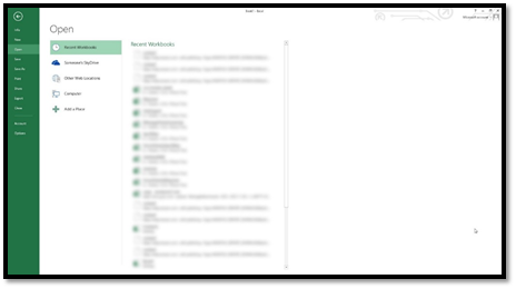
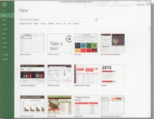
Start Screen in MS Excel 2013
How do you access spreadsheets, use templates, and disable the Screen in Excel?
Let’s start this Excel 2013 Tutorial by navigating the new Start Screen in Excel 2013, which allows you to work more efficiently. If you want to access worksheets you have used recently, they can be found on the left edge of the screen. In addition, you can even pin these worksheets to the “Recent” list so you can view them at all times. You can also click “Open Other Workbooks” to open files from the cloud or external storage such as a disk. To access Excel in the cloud, you can find your SkyDrive cloud storage account on the top right edge of the screen.
If you want to start a project right away, Excel 2013 provides various templates on the screen that you can choose from, along with enabling you to search the internet for more templates. Excel also provides a list of suggestions in case you are not sure about which template to use. If you find a template suitable, you can pin it for easy future access as well.
We have included a screen capture from the newly designed Start Menu in Excel 2013 right below.
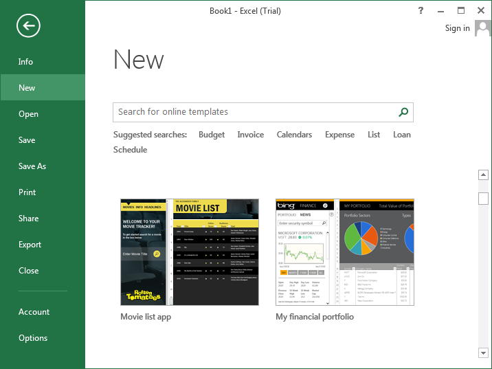
Users who have limited or no experience working with Microsoft Excel will especially benefit from the template options, while regular users will appreciate the “Recent” file list along with hassle free access. Note that while the Start Screen presents a host of benefits, you can even disable it if necessary.
To disable the start screen in Excel 13, open a new document and go to “File”, followed by “Options”. Unselect “Show the Start Screen when this application starts” in the “Start up options”.
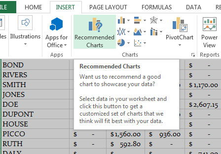
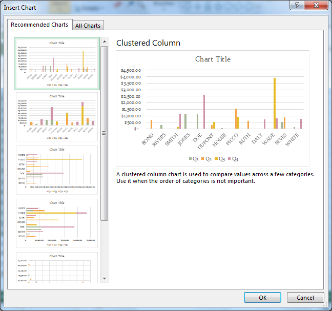
Recommended Charts – How to Select, Insert, and Format
Next the “Recommended Charts” new feature in Excel 2013 illustrates the fact that while fresh features have been incorporated in Excel 2013, they do not meddle with the usability. Basically this intuitive option displays just the breakup of chart types that maybe relevant to the information you have entered in Excel. So even if you are not good with making charts, this feature will help you find the most suitable one without barging in the whole screen.
Here in this Excel 2013 Tutorial, we show how you can use this tool. Highlight the information that you want to work on in MS Excel 2013. Next, click “Insert”, followed by “Recommended Charts”. You will now see a dialog box on the screen which has all the chart options. If you click on a chart, you will have a preview of how the data will appear on it. To create a Chart, simply click “OK” and your work will be done.
If you remember from the earlier Excel versions, selecting a chart would make 3 extra tabs appear in the Chart Tools tab. These were Design, Layout, and Format. Now you only have the Design and Format tabs which make the interface of Excel less cluttered. Not to mention, you will also have an additional set of icons on the top right corner of the chart you select.
These related buttons in Microsoft Excel 2013 are “Chart Elements”, “Chart Styles”, and “Chart Filters”, and pressing them enables you to use extra formatting options. For instance, by using “Chart Elements” you can add or remove elements like axis titles, whereas with “Chart Styles” you can change the color of the chart. Finally, filtered data can be viewed with live preview via “Chart Filters”.
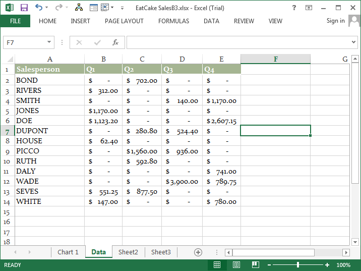
The next three graphic images illustrate how Recommended Charts can be beneficial in quickly analyzing Sales by Quarter information for your team. The first image simply has the data for each quarter by our Sales staff.
Pivot Tables – How to Insert them?
Next item in this Excel 2013 training article is Pivot Tables. These tables are a great feature to help experienced users analyze their data. Note that if you if have not used Excel previously, you will find it hard to create Pivot Tables. However, Excel 2013 has the “Recommended PivotTables” option to get you started. Here is how you can use this option.
Select the entire data (headings included), and then do the following:
Select “Insert” > “Recommended PivotTables” You will now see a dialog box that displays a sequence of PivotTables that analyze and explain the data. To create a PivotTable automatically, simply click “OK”.
Backstage View – How to View and Pin Files
The Backstage View was first launched in Office 2010. To access it in Excel 2013, simply go the File menu. Note that this feature has been improved in Excel 2013 to help you select the correct task. You can even view your recently used Exel workbooks from the “Open Tab” which serves the dual purpose of the “Open” and “Recent” options in the 2010 version of Excel.
You can pin frequently used worksheets to this list and you can click “Computer” to access and pin recently visited locations. You can even access your SkyDrive (online storage), plus add other accounts for cloud storage as well.
Quick Analysis – Use This Tool to Format your Data
We move on to Quick Analysis as we continue with this Microsoft Excel 2013 training. Here is another tool to help you work smoothly on MS Excel 2013 by helping you look for formatting options to use on your data. This is how you can enable the Quick Analysis tool. Highlight your data, and you will find the Quick Analysis icon in the bottom right corner of your data. When you click the icon, a dialog will come into view that will display a variety of tools such as “Formatting”, “Tables”, and “Sparklines”.
These tools will help you analyze the data in MS Office Excel. If you click on these options, another sequence of functions will come into view and you can preview each one by hovering the cursor over them. If you want to use any of the options, simply click on it. This makes tasks like formatting or adding formulas speedier than before.
This is shown from the following screen capture in Excel 2013.

Related Resources on Excel 2013 Training
– Free MS Excel 2013 Tutorial
– Training courses for Excel
– 10 New Features in Microsoft Excel 2013 – YouTube
– Try Office 2013 video training for FREE!
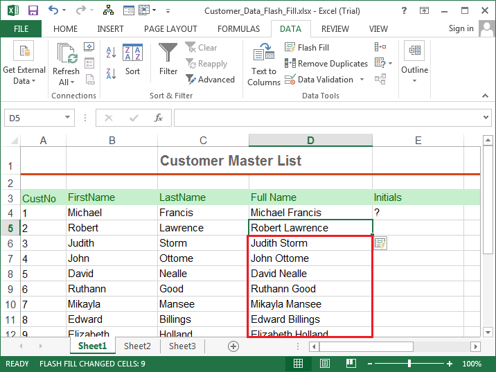
Flash Fill – How to Add or Extract Data
Flash Fill is perhaps the best new tool you will find in Microsoft Excel 2013. The Flash Fill new feature identifies patterns that you use regularly and then adds or removes data automatically in the same sequence. Using Flash Fill in Excel 2013, you can manage some common problems that are not easy to come around manually. For instance, let’s say you have a list of American cities with the name of the state alongside. However, you have to extract just a city’s name from the column.
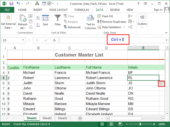
Simply go the next blank column along with one that contains both the city and its state, and type the city’s name. Next, click “Home”, followed by “Fill” and “Flash Fill”. The blank column will now display just the names of the city. In the same way in Excel 2013, you can add or extract contact details of people, and even extract specific numerical data from the cells. Of course, you can do this with formulas as well, but the Flash Fill makes the process simpler and quicker.
Here in this Excel 2013 tutorial, we have an example of Flash Fill, Excel 2013 new cool feature in Action. We have a list of customers with first and last names. We would like to do the following:
- Combine the first and last name into a Full Name – Column
- Extract the Initials from the Full Name – Column


Power View – How to Create Quick Analysis for Sizeable Data
Next in our Excel 2013 lesson, we are going to look at Power View. Excel 2013 retains the Power View add-in from its predecessors. This add-in is basically utilized for analyzing large chunks of information that has been added via external sources. Power View therefore is a great resource for creating reports in large organizations. To see this tool in action, select the data you want Excel to analyze and then choose
“Insert”, followed by “Power View”.
Note that when you use this for the first time, the Power View installs automatically. Next, a Power View sheet will be added to your Excel 2013 workbook, creating an analysis report on the data you selected. Once the report is created, you can add titles, filter the data, and change its display. To access format options, go to the Ribbon toolbar and select the Power View tab. You will find options like “Theme and text” formats, View options, and Filters Area.
This is what Power View in MS Excel 2013 looks like.

How to Create a Sample Spreadsheet
Considering all the information given above, here is how you can create a basic workbook or spreadsheet on Excel 2013.
To create a new Excel workbook, go to:
File > Click New > Blank workbook
To enter data, you need to click on cells, which are arranged according to their location in row and column. For example, A3. Once you click on a cell, enter text or numerical data and press the Enter or Tab to proceed to the next cell.
To add numbers on your sheet, select a cell on the right or beneath the numbers that have to be added. Select “Home” followed by “AutoSum”. Alternately, you can use the keyboard shortcut Alt +=. Moving on, when you type in = in a cell, Excel recognized that this cell will contain a formula. Using other signs like +,-,*(for multiplication), and / (for division), you can simply press Enter to get the results on any sum. To keep the cursor active on a particular cell, press Ctrl+Enter.
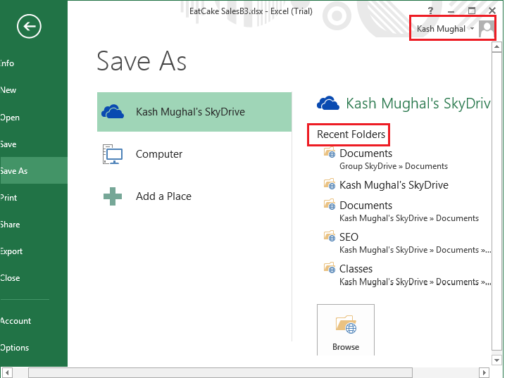
To organize the Excel 2013 data in a meaningful manner, you can use the features mentioned above, such as the Quick Analysis tool and PivotTables. Finally, you can save this workbook on the Web. Sign in to your Microsoft account (Hotmail, Messenger, or Xbox Live). Open the workbook, click “File” and select “Save As”.
Select “Add a Place” followed by “SkyDrive”. Use “Microsoft account” to sign in. Enter account details and click “Sign In”. Now you will find your SkyDrive under the “Places” section. Click “Places”, followed by “Recent Folders”. If you still don’t see your folder, select “Browse for Additional Folders”. Enter the name of your Excel file, and click “Save”.
Next in this Excel 2013 training, lets go ahead and save the EatCake spreadsheet to the SkyDrive that we were working on earlier. If not already signed into SkyDrive yet, you need to click on the Sign In button (top right). After you have logged into you account (get yours at http://www.live.com), you will see a new option. Now you can see option to save to your SkyDrive and even the folders/directories in the cloud. When we tried to save the file, we go the following options:
How to Share your Office 2013 Excel Work
Once you have used to the above-mentioned features to organize your data, you can share your work with colleagues and friends in real time, which is yet another fascinating aspect of MS Excel 2013. Using the Excel WebApp, files can be shared and worked upon by others through SkyDrive. Note that if 2 people try to perform the same action on one file simultaneously, you can experience some problems.
Moreover, if someone else is working on a Microsoft Excel worksheet, you cannot open it from SkyDrive on your device. This limitation ensures that there are no conflicting changes in the same file. However, if an Excel file that is stored online is being used by someone, you can (with permission) download or view it. But none of the changes you make will be reflected in the original file which will remain locked unless the other person closes it.
Also remember that the new Excel 2013, like all other applications in Office 2013, automatically saves files to the cloud which you can access through the a browser with the Excel WebApp even if you do not have Excel on your local hard drive.
Moving on in this Excel 2013 lesson, you can even share files via social network direct from Excel 2013. To share your files on networks like Facebook, start by saving them to SkyDrive first. If you haven’t done so, simply click “File” followed by “Share”, and then select “Invite People”. In this way, you will come across “Save As” options in a while.
After this process, you will return back to the Share panel where you see “Post to Social Networks”. You can choose any social network provided that it is linked with your Office 2013 account. Here you can include a message and decide whether others can edit the worksheet you are sharing. After doing this, your post is ready to be shared.
You can even share Excel 2013 sheets in online meetings. Even if you are not at work, you can simply connect and share workbooks using a smartphone or tablet. However, you need to have Lync installed on your device. To use this feature, first close down any files you do not want to share. Next, click “File” followed by “Share”, and “Present Online”. Finally, click “Present”.
If Lync is not running, you have to sign in to continue. In the “Shared Workbook Window” section, select between a planned meetingor “Start a new Lync meeting”, followed by OK. You can bring in more people to the online meeting by clicking the “Participants” button and selecting “Invite More People”. You can select contacts from the list or enter their names manually. If you need to stop sharing with Lync, simply click “Stop Sharing” at the top of the Screen.
These were the major functions you can perform on the Excel 2013.
Excel 2013 Tutorial – Related Links:
For those who require additional training on MS Excel 2013, then the following links may be good ones to check out:
–What’s new in Excel 2013
–Securing documents in Office 2013
–10 Awesome new features in Excel 2013
–Microsoft Excel 2010 Tutorial
If you are after getting more information about Excel 2013 then the link below is a useful one to look into.
http://office.microsoft.com/en-us/excel/
Connect with US!
![]()