Contents
- 1 Introduction
- 2 What is Word Embeddings?
- 3 What is Word2Vec Model?
- 4 Word2Vec Architecture
- 4.1 i) Continuous Bag of Words (CBOW) Model
- 4.2 ii) Skip-Gram Model
- 4.3 CBOW vs Skip-Gram Word2Vec Model
- 5 Word2Vec using Gensim Library
- 5.1 Installing Gensim Library
- 6 Working with Pretrained Word2Vec Model in Gensim
- 6.1 i) Download Pre-Trained Weights
- 6.2 ii) Load Libraries
- 6.3 iii) Load Pre-Trained Weights
- 6.4 iv) Checking Vectors of Words
- 6.5 iv) Most Similar Words
- 6.6 v) Word Analogies
- 7 Training Custom Word2Vec Model in Gensim
- 7.1 i) Understanding Syntax of Word2Vec()
- 7.2 ii) Dataset for Custom Training
- 7.3 iii) Loading Libraries
- 7.4 iii) Loading of Dataset
- 7.5 iv) Text Preprocessing
- 7.6 v) Train CBOW Word2Vec Model
- 7.7 v) Train Skip-Gram Word2Vec Model
- 7.8 v) Visualizing Word Embeddings
- 7.8.1 a) Visualize Word Embeddings for CBOW
- 7.8.2 b) Visualize Word Embeddings for Skip-Gram
Introduction
In this article, we will see the tutorial for doing word embeddings with the word2vec model in the Gensim library. We will first understand what is word embeddings and what is word2vec model. Then we will see its two types of architectures namely the Continuous Bag of Words (CBOW) model and Skip Gram model. Finally, we will explain how to use the pre-trained word2vec model and how to train a custom word2vec model in Gensim with your own text corpus. And as a bonus, we will also cover the visualization of our custom word2vec model.
What is Word Embeddings?
Machine learning and deep learning algorithms cannot work with text data directly, hence they need to be converted into numerical representations. In NLP, there are techniques like Bag of Words, Term Frequency, TF-IDF, to convert text into numeric vectors. However, these classical techniques do not represent the semantic relationship relationships between the texts in numeric form.
This is where word embedding comes into play. Word Embeddings are numeric vector representations of text that also maintain the semantic and contextual relationships within the words in the text corpus.
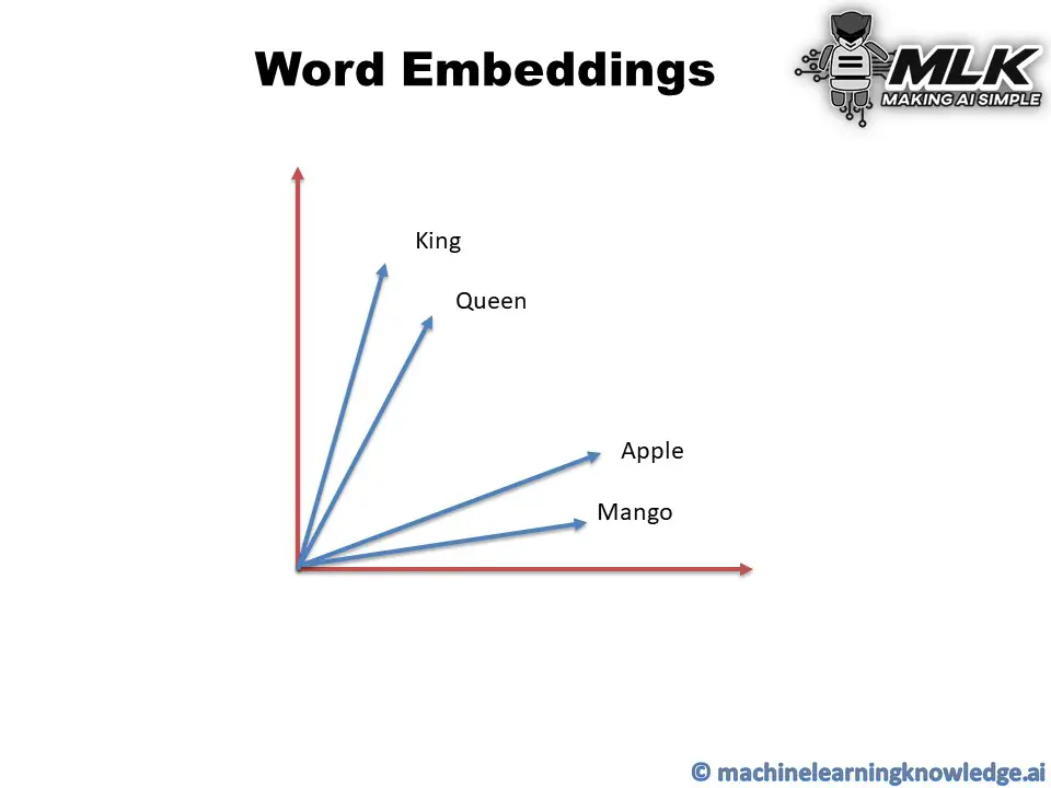
In such representation, the words that have stronger semantic relationships are closer to each other in the vector space. As you can see in the below example, the words Apple and Mango are close to each other as they both have many similar features of being fruit. Similarly, the words King and Queen are close to each other because they are similar in the royal context.
Ad
What is Word2Vec Model?
Word2vec is a popular technique for creating word embedding models by using neural network. The word2vec architectures were proposed by a team of researchers led by Tomas Mikolov at Google in 2013.
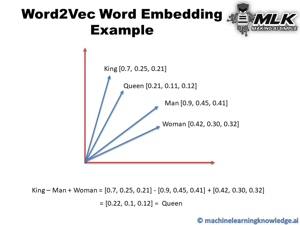
The word2vec model can create numeric vector representations of words from the training text corpus that maintains the semantic and syntactic relationship. A very famous example of how word2vec preserves the semantics is when you subtract the word Man from King and add Woman it gives you Queen as one of the closest results.
King – Man + Woman ≈ Queen
You may think about how we are doing addition or subtraction with words but do remember that these words are represented by numeric vectors in word2vec so when you apply subtraction and addition the resultant vector is closer to the vector representation of Queen.
In vector space, the word pair of King and Queen and the pair of Man and Woman have similar distances between them. This is another way putting that word2vec can draw the analogy that if Man is to Woman then Kind is to Queen!
The publicly released model of word2vec by Google consists of 300 features and the model is trained in the Google news dataset. The vocabulary size of the model is around 1.6 billion words. However, this might have taken a huge time for the model to be trained on but they have applied a method of simple subsampling approach to optimize the time.
Word2Vec Architecture
The paper proposed two word2vec architectures to create word embedding models – i) Continuous Bag of Words (CBOW) and ii) Skip-Gram.
i) Continuous Bag of Words (CBOW) Model
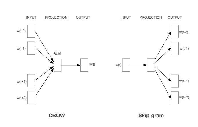
In the continuous bag of words architecture, the model predicts the current word from the surrounding context words. The length of the surrounding context word is the window size that is a tunable hyperparameter. The model can be trained by a single hidden layer neural network.
Once the neural network is trained, it results in the vector representation of the words in the training corpus. The size of the vector is also a hyperparameter that we can accordingly choose to produce the best possible results.
ii) Skip-Gram Model
In the skip-gram model, the neural network is trained to predict the surrounding context words given the current word as input. Here also the window size of the surrounding context words is a tunable parameter.
When the neural network is trained, it produces the vector representation of the words in the training corpus. Hera also the size of the vector is a hyperparameter that can be experimented with to produce the best results.
CBOW vs Skip-Gram Word2Vec Model
- CBOW model is trained by predicting the current word by giving the surrounding context words as input. Whereas the Skip-Gram model is trained by predicting the surrounding context words by providing the central word as input.
- CBOW model is faster to train as compared to the Skip-Gram model.
- CBOW model works well to represent the more frequently appearing words whereas Skip-Gram works better to represent less frequent rare words.
For details and information, you may refer to the original word2vec paper here.
Word2Vec using Gensim Library
Gensim is an open-source python library for natural language processing. Working with Word2Vec in Gensim is the easiest option for beginners due to its high-level API for training your own CBOW and SKip-Gram model or running a pre-trained word2vec model.
Installing Gensim Library
Let us install the Gensim library and its supporting library python-Levenshtein.
In[1]:
pip install gensim
pip install python-Levenshtein
In the below sections, we will show you how to run the pre-trained word2vec model in Gensim and then show you how to train your CBOW and SKip-Gram.
(All the examples are shown with Genism 4.0 and may not work with Genism 3.x version)
Working with Pretrained Word2Vec Model in Gensim
i) Download Pre-Trained Weights
We will use the pre-trained weights of word2vec that was trained on Google New corpus containing 3 billion words. This model consists of 300-dimensional vectors for 3 million words and phrases.
The weight can be downloaded from this link. It is a 1.5GB file so make sure you have enough space to save it.
ii) Load Libraries
We load the required Gensim libraries and modules as shown below –
In[2]:
import gensim
from gensim.models import Word2Vec,KeyedVectors
iii) Load Pre-Trained Weights
Next, we load our pre-trained weights by using the KeyedVectors.load_word2vec_format() module of Gensim. Make sure to give the right path of pre-trained weights in the first parameter. (In our case, it is saved in the current working directory)
In[3]:
model = KeyedVectors.load_word2vec_format('GoogleNews-vectors-negative300.bin.gz',binary=True,limit=100000)
iv) Checking Vectors of Words
We can check the numerical vector representation just like the below example where we have shown it for the word man.
In[4]:
vec = model['man']
print(vec)
Out[4]:
[ 0.32617188  0.13085938  0.03466797 -0.08300781  0.08984375 -0.04125977
 -0.19824219  0.00689697  0.14355469  0.0019455   0.02880859 -0.25
 -0.08398438 -0.15136719 -0.10205078  0.04077148 -0.09765625  0.05932617
  0.02978516 -0.10058594 -0.13085938  0.001297    0.02612305 -0.27148438
  0.06396484 -0.19140625 -0.078125    0.25976562  0.375      -0.04541016
  0.16210938  0.13671875 -0.06396484 -0.02062988 -0.09667969  0.25390625
  0.24804688 -0.12695312  0.07177734  0.3203125   0.03149414 -0.03857422
  0.21191406 -0.00811768  0.22265625 -0.13476562 -0.07617188  0.01049805
 -0.05175781  0.03808594 -0.13378906  0.125       0.0559082  -0.18261719
  0.08154297 -0.08447266 -0.07763672 -0.04345703  0.08105469 -0.01092529
  0.17480469  0.30664062 -0.04321289 -0.01416016  0.09082031 -0.00927734
 -0.03442383 -0.11523438  0.12451172 -0.0246582   0.08544922  0.14355469
 -0.27734375  0.03662109 -0.11035156  0.13085938 -0.01721191 -0.08056641
 -0.00708008 -0.02954102  0.30078125 -0.09033203  0.03149414 -0.18652344
 -0.11181641  0.10253906 -0.25976562 -0.02209473  0.16796875 -0.05322266
 -0.14550781 -0.01049805 -0.03039551 -0.03857422  0.11523438 -0.0062561
 -0.13964844  0.08007812  0.06103516 -0.15332031 -0.11132812 -0.14160156
  0.19824219 -0.06933594  0.29296875 -0.16015625  0.20898438  0.00041771
  0.01831055 -0.20214844  0.04760742  0.05810547 -0.0123291  -0.01989746
 -0.00364685 -0.0135498  -0.08251953 -0.03149414  0.00717163  0.20117188
  0.08300781 -0.0480957  -0.26367188 -0.09667969 -0.22558594 -0.09667969
  0.06494141 -0.02502441  0.08496094  0.03198242 -0.07568359 -0.25390625
 -0.11669922 -0.01446533 -0.16015625 -0.00701904 -0.05712891  0.02807617
 -0.09179688  0.25195312  0.24121094  0.06640625  0.12988281  0.17089844
 -0.13671875  0.1875     -0.10009766 -0.04199219 -0.12011719  0.00524902
  0.15625    -0.203125   -0.07128906 -0.06103516  0.01635742  0.18261719
  0.03588867 -0.04248047  0.16796875 -0.15039062 -0.16992188  0.01831055
  0.27734375 -0.01269531 -0.0390625  -0.15429688  0.18457031 -0.07910156
  0.09033203 -0.02709961  0.08251953  0.06738281 -0.16113281 -0.19628906
 -0.15234375 -0.04711914  0.04760742  0.05908203 -0.16894531 -0.14941406
  0.12988281  0.04321289  0.02624512 -0.1796875  -0.19628906  0.06445312
  0.08935547  0.1640625  -0.03808594 -0.09814453 -0.01483154  0.1875
  0.12792969  0.22753906  0.01818848 -0.07958984 -0.11376953 -0.06933594
 -0.15527344 -0.08105469 -0.09277344 -0.11328125 -0.15136719 -0.08007812
 -0.05126953 -0.15332031  0.11669922  0.06835938  0.0324707  -0.33984375
 -0.08154297 -0.08349609  0.04003906  0.04907227 -0.24121094 -0.13476562
 -0.05932617  0.12158203 -0.34179688  0.16503906  0.06176758 -0.18164062
  0.20117188 -0.07714844  0.1640625   0.00402832  0.30273438 -0.10009766
 -0.13671875 -0.05957031  0.0625     -0.21289062 -0.06542969  0.1796875
 -0.07763672 -0.01928711 -0.15039062 -0.00106049  0.03417969  0.03344727
  0.19335938  0.01965332 -0.19921875 -0.10644531  0.01525879  0.00927734
  0.01416016 -0.02392578  0.05883789  0.02368164  0.125       0.04760742
 -0.05566406  0.11572266  0.14746094  0.1015625  -0.07128906 -0.07714844
 -0.12597656  0.0291748   0.09521484 -0.12402344 -0.109375   -0.12890625
  0.16308594  0.28320312 -0.03149414  0.12304688 -0.23242188 -0.09375
 -0.12988281  0.0135498  -0.03881836 -0.08251953  0.00897217  0.16308594
  0.10546875 -0.13867188 -0.16503906 -0.03857422  0.10839844 -0.10498047
  0.06396484  0.38867188 -0.05981445 -0.0612793  -0.10449219 -0.16796875
  0.07177734  0.13964844  0.15527344 -0.03125    -0.20214844 -0.12988281
 -0.10058594 -0.06396484 -0.08349609 -0.30273438 -0.08007812  0.02099609]
iv) Most Similar Words
We can get the list of words similar to the given words by using the most_similar() API of Gensim.
In[5]:
model.most_similar('man')
Out[5]:
[(‘woman’, 0.7664012908935547),
(‘boy’, 0.6824871301651001),
(‘teenager’, 0.6586930155754089),
(‘teenage_girl’, 0.6147903203964233),
(‘girl’, 0.5921714305877686),
(‘robber’, 0.5585119128227234),
(‘teen_ager’, 0.5549196600914001),
(‘men’, 0.5489763021469116),
(‘guy’, 0.5420035123825073),
(‘person’, 0.5342026352882385)]
In[6]:
model.most_similar('PHP')
Out[6]:
[(‘ASP.NET’, 0.7275794744491577),
(‘Visual_Basic’, 0.6807329654693604),
(‘J2EE’, 0.6805503368377686),
(‘Drupal’, 0.6674476265907288),
(‘NET_Framework’, 0.6344218254089355),
(‘Perl’, 0.6339991688728333),
(‘MySQL’, 0.6315538883209229),
(‘AJAX’, 0.6286270618438721),
(‘plugins’, 0.6174636483192444),
(‘SQL’, 0.6123985052108765)]
v) Word Analogies
Let us now see the real working example of King-Man+Woman of word2vec in the below example. After doing this operation we use most_similar() API and can see Queen is at the top of the similarity list.
In[7]:
vec = model['king'] - model['man'] + model['women']
model.most_similar([vec])
Out[7]:
[(‘king’, 0.6478992700576782),
(‘queen’, 0.535493791103363),
(‘women’, 0.5233659148216248),
(‘kings’, 0.5162314772605896),
(‘queens’, 0.4995364248752594),
(‘princes’, 0.46233269572257996),
(‘monarch’, 0.45280295610427856),
(‘monarchy’, 0.4293173849582672),
(‘crown_prince’, 0.42302510142326355),
(‘womens’, 0.41756653785705566)]
Let us see another example, this time we do INR – India + England and amazingly the model returns the currency GBP in the most_similar results.
In[8]:
vec = model['INR'] - model ['India'] + model['England']
model.most_similar([vec])
Out[8]:
[(‘INR’, 0.6442341208457947),
(‘GBP’, 0.5040826797485352),
(‘England’, 0.44649264216423035),
(‘£’, 0.43340998888015747),
(‘Â_£’, 0.4307197630405426),
(‘£_#.##m’, 0.42561301589012146),
(‘GBP##’, 0.42464491724967957),
(‘stg’, 0.42324796319007874),
(‘EUR’, 0.418365478515625),
(‘€’, 0.4151178002357483)]
Training Custom Word2Vec Model in Gensim
i) Understanding Syntax of Word2Vec()
It is very easy to train custom wor2vec model in Gensim with your own text corpus by using Word2Vec() module of gensim.models by providing the following parameters –
- sentences: It is an iterable list of tokenized sentences that will serve as the corpus for training the model.
- min_count: If any word has a frequency below this, it will be ignored.
- workers: Number of CPU worker threads to be used for training the model.
- window: It is the maximum distance between the current and predicted word considered in the sentence during training.
- sg: This denotes the training algorithm. If sg=1 then skip-gram is used for training and if sg=0 then CBOW is used for training.
- epochs: Number of epochs for training.
These are just a few parameters that we are using, but there are many other parameters available for more flexibility. For full syntax check the Gensim documentation here.
ii) Dataset for Custom Training
For the training purpose, we are going to use the first book of the Harry Potter series – “The Philosopher’s Stone”. The text file version can be downloaded from this link.
iii) Loading Libraries
We will be loading the following libraries. TSNE and matplotlib are loaded to visualize the word embeddings of our custom word2vec model.
In[9]:
# For Data Preprocessing
import pandas as pd

# Gensim Libraries
import gensim
from gensim.models import Word2Vec,KeyedVectors

# For visualization of word2vec model
from sklearn.manifold import TSNE
import matplotlib.pyplot as plt
%matplotlib inline
iii) Loading of Dataset
Next, we load the dataset by using the pandas read_csv function.
In[10]:
df = pd.read_csv('HarryPotter.txt', delimiter = "n",header=None)
df.columns = ['Line']
df
Out[10]:
| Line | |
|---|---|
| 0 | / |
| 1 | THE BOY WHO LIVED |
| 2 | Mr. and Mrs. Dursley, of number four, Privet D… |
| 3 | were proud to say that they were perfectly nor… |
| 4 | thank you very much. They were the last people… |
| … | … |
| 6757 | “Oh, I will,” said Harry, and they were surpri… |
| 6758 | the grin that was spreading over his face. “ T… |
| 6759 | know we’re not allowed to use magic at home. I’m |
| 6760 | going to have a lot of fun with Dudley this su… |
| 6761 | Page | 348 |
6762 rows × 1 columns
iv) Text Preprocessing
For preprocessing we are going to use gensim.utils.simple_preprocess that does the basic preprocessing by tokenizing the text corpus into a list of sentences and remove some stopwords and punctuations.
gensim.utils.simple_preprocess module is good for basic purposes but if you are going to create a serious model, we advise using other standard options and techniques for robust text cleaning and preprocessing.
- Also Read – 11 Techniques of Text Preprocessing Using NLTK in Python
In[11]:
preprocessed_text = df['Line'].apply(gensim.utils.simple_preprocess)
preprocessed_text
Out[11]:
0                                                      []
1                                  [the, boy, who, lived]
2       [mr, and, mrs, dursley, of, number, four, priv...
3       [were, proud, to, say, that, they, were, perfe...
4       [thank, you, very, much, they, were, the, last...
                              ...
6757    [oh, will, said, harry, and, they, were, surpr...
6758    [the, grin, that, was, spreading, over, his, f...
6759    [know, we, re, not, allowed, to, use, magic, a...
6760    [going, to, have, lot, of, fun, with, dudley, ...
6761                                               [page]
Name: Line, Length: 6762, dtype: object
v) Train CBOW Word2Vec Model
This is where we train the custom word2vec model with the CBOW technique. For this, we pass the value of sg=0 along with other parameters as shown below.
The value of other parameters is taken with experimentations and may not produce a good model since our goal is to explain the steps for training your own custom CBOW model. You may have to tune these hyperparameters to produce good results.
In[12]:
model_cbow = Word2Vec(sentences=preprocessed_text, sg=0, min_count=10, workers=4, window =3, epochs = 20)
Once the training is complete we can quickly check an example of finding the most similar words to “harry”. It actually does a good job to list out other character’s names that are close friends of Harry Potter. Is it not cool!
In[13]:
model_cbow.wv.most_similar("harry")
Out[13]:
[(‘ron’, 0.8734568953514099),
(‘neville’, 0.8471445441246033),
(‘hermione’, 0.7981335520744324),
(‘hagrid’, 0.7969962954521179),
(‘malfoy’, 0.7925101518630981),
(‘she’, 0.772059977054596),
(‘seamus’, 0.6930352449417114),
(‘quickly’, 0.692932665348053),
(‘he’, 0.691251814365387),
(‘suddenly’, 0.6806278228759766)]
v) Train Skip-Gram Word2Vec Model
For training word2vec with skip-gram technique, we pass the value of sg=1 along with other parameters as shown below. Again, these hyperparameters are just for experimentation and you may like to tune them for better results.
In[14]:
model_skipgram = Word2Vec(sentences =preprocessed_text, sg=1, min_count=10, workers=4, window =10, epochs = 20)
Again, once training is completed, we can check how this model works by finding the most similar words for “harry”. But this time we see the results are not as impressive as the one with CBOW.
In[15]:
model_skipgram.wv.most_similar("harry")
Out[15]:
[(‘goblin’, 0.5757830142974854),
(‘together’, 0.5725131630897522),
(‘shaking’, 0.5482161641120911),
(‘he’, 0.5105234980583191),
(‘working’, 0.5037856698036194),
(‘the’, 0.5015968084335327),
(‘page’, 0.4912668466567993),
(‘story’, 0.4897386431694031),
(‘furiously’, 0.4880291223526001),
(‘then’, 0.47639384865760803)]
v) Visualizing Word Embeddings
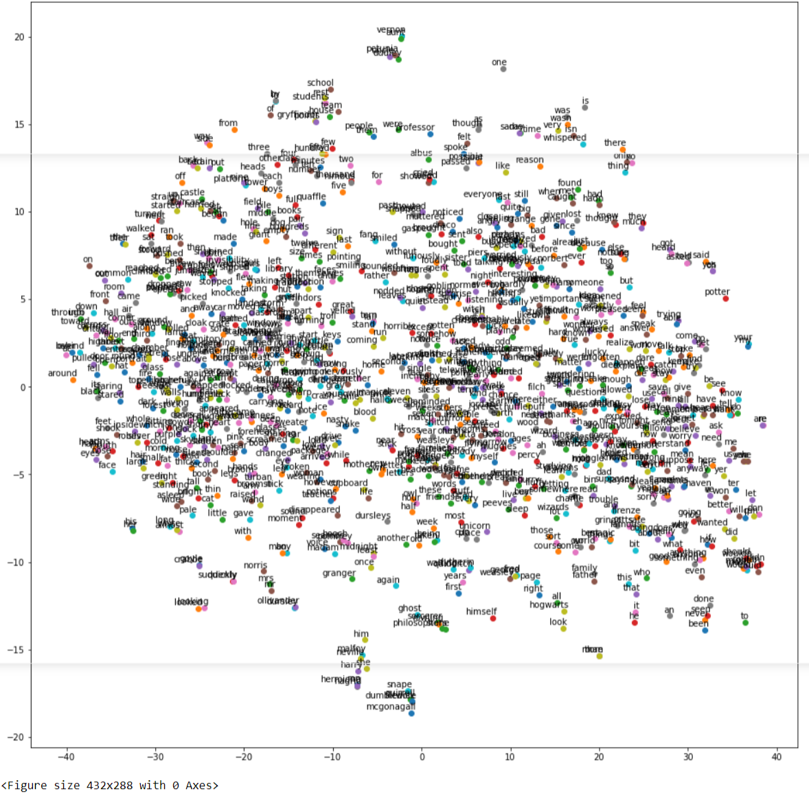
The word embedding model created by wor2vec can be visualized by using Matplotlib and the TNSE module of Sklearn. The below code has been referenced from the Kaggle code by Jeff Delaney here and we have just modified the code to make it compatible with Gensim 4.0 version.
In[16]:
def tsne_plot(model):
    "Creates and TSNE model and plots it"
    labels = []
    tokens = []

    for word in model.wv.key_to_index:

        tokens.append(model.wv[word])
        labels.append(word)

    tsne_model = TSNE(perplexity=40, n_components=2, init='pca', n_iter=2500, random_state=23)
    new_values = tsne_model.fit_transform(tokens)

    x = []
    y = []
    for value in new_values:
        x.append(value[0])
        y.append(value[1])

    plt.figure(figsize=(16, 16))
    for i in range(len(x)):
        plt.scatter(x[i],y[i])
        plt.annotate(labels[i],
                     xy=(x[i], y[i]),
                     xytext=(5, 2),
                     textcoords='offset points',
                     ha='right',
                     va='bottom')
    plt.show()
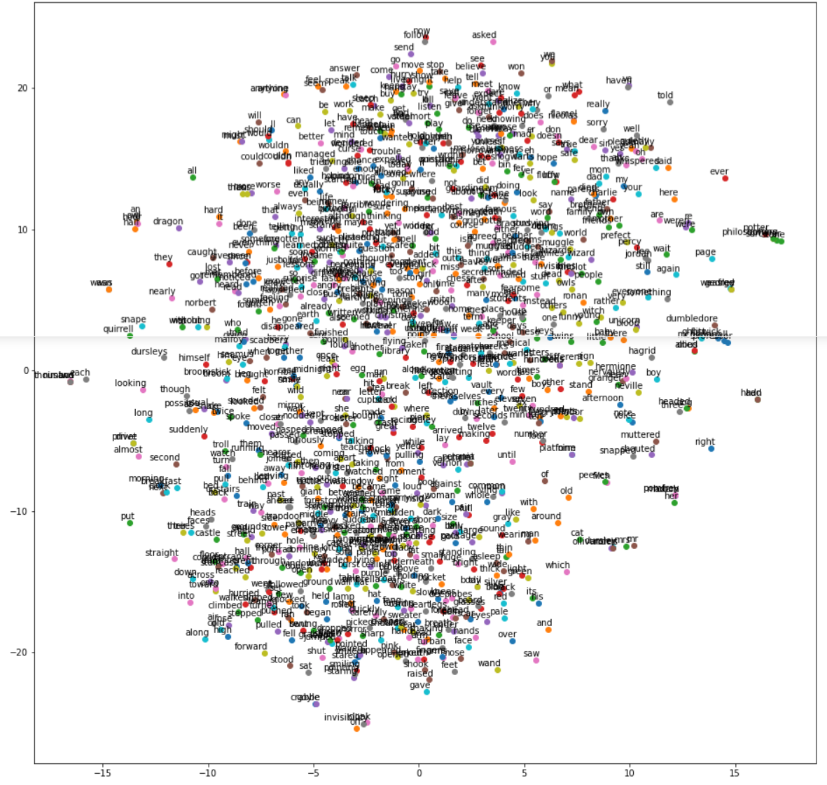
a) Visualize Word Embeddings for CBOW
Let us visualize the word embeddings of our custom CBOW model by using the above custom function.
In[17]:
tsne_plot(model_cbow)
Out[17]:
b) Visualize Word Embeddings for Skip-Gram
Let us visualize the word embeddings of our custom Skip-Gram model by using the above custom function.
In[18]:
tsne_plot(model_skipgram)
Out[18]:
A Hands-On Word2Vec Tutorial Using the Gensim Package
The idea behind Word2Vec is pretty simple. We’re making an assumption that the meaning of a word can be inferred by the company it keeps. This is analogous to the saying, “show me your friends, and I’ll tell who you are”.
If you have two words that have very similar neighbors (meaning: the context in which it’s used is about the same), then these words are probably quite similar in meaning or are at least related. For example, the words shocked, appalled and astonished are usually used in a similar context.
“The meaning of a word can be inferred by the company it keeps”
Using this underlying assumption, you can use Word2Vec to:
- Surface similar concepts
- Find unrelated concepts
- Compute similarity between two words and more!
Getting Started with the Gensim Word2Vec Tutorial
In this tutorial, you will learn how to use the Gensim implementation of Word2Vec (in python) and actually get it to work! I‘ve long heard complaints about poor performance, but it really is a combination of two things: (1) your input data and (2) your parameter settings. Check out the Jupyter Notebook if you want direct access to the working example, or read on to get more context.
Side note: The training algorithms in the Gensim package were actually ported from the original Word2Vec implementation by Google and extended with additional functionality.
Imports and logging
First, we start with our imports and get logging established:
# imports needed and logging
import gzip
import gensim
import logging

logging.basicConfig(format=’%(asctime)s : %(levelname)s : %(message)s’, level=logging.INFO)
Dataset
Next, is finding a really good dataset. The secret to getting Word2Vec really working for you is to have lots and lots of text data in the relevant domain. For example, if your goal is to build a sentiment lexicon, then using a dataset from the medical domain or even wikipedia may not be effective. So, choose your dataset wisely. As Matei Zaharia says,
It’s your data, stupid
That was said in the context of data quality, but it’s not just quality it’s also using the right data for the task.
For this Gensim Word2Vec tutorial, I am going to use data from the OpinRank dataset from some of my Ph.D work. This dataset has full user reviews of cars and hotels. I have specifically concatenated all of the hotel reviews into one big file which is about 97 MB compressed and 229 MB uncompressed. We will use the compressed file for this tutorial. Each line in this file represents a hotel review.
Now, let’s take a closer look at this data below by printing the first line.
with gzip.open (input_file, 'rb') as f:
        for i,line in enumerate (f):
            print(line)
            break
You should see the following:
b"Oct 12 2009 tNice trendy hotel location not too bad.tI stayed in this hotel for one night. As this is a fairly new place some of the taxi drivers did not know where it was and/or did not want to drive there. Once I have eventually arrived at the hotel, I was very pleasantly surprised with the decor of the lobby/ground floor area. It was very stylish and modern. I found the reception's staff geeting me with 'Aloha' a bit out of place, but I guess they are briefed to say that to keep up the coroporate image.As I have a Starwood Preferred Guest member, I was given a small gift upon-check in. It was only a couple of fridge magnets in a gift box, but nevertheless a nice gesture.My room was nice and roomy, there are tea and coffee facilities in each room and you get two complimentary bottles of water plus some toiletries by 'bliss'.The location is not great. It is at the last metro stop and you then need to take a taxi, but if you are not planning on going to see the historic sites in Beijing, then you will be ok.I chose to have some breakfast in the hotel, which was really tasty and there was a good selection of dishes. There are a couple of computers to use in the communal area, as well as a pool table. There is also a small swimming pool and a gym area.I would definitely stay in this hotel again, but only if I did not plan to travel to central Beijing, as it can take a long time. The location is ok if you plan to do a lot of shopping, as there is a big shopping centre just few minutes away from the hotel and there are plenty of eating options around, including restaurants that serve a dog meat!trn"
You can see that this is a pretty good full review with many words and that’s what we want. We have approximately 255,000 such reviews in this dataset.
To avoid confusion, the Gensim’s Word2Vec tutorial says that you need to pass a list of tokenized sentences as the input to Word2Vec. However, you can actually pass in a whole review as a sentence (i.e. a much larger size of text), if you have a lot of data and it should not make much of a difference. In the end, all we are using the dataset for is to get all neighboring words (the context) for a given target word.
Read files into a list
Now that we’ve had a sneak peak of our dataset, we can read it into a list so that we can pass this on to the Word2Vec model. Notice in the code below, that I am directly reading the compressed file. I’m also doing a mild pre-processing of the reviews using gensim.utils.simple_preprocess (line). This does some basic pre-processing such as tokenization, lowercasing, etc. and returns back a list of tokens (words). Documentation of this pre-processing method can be found on the official Gensim documentation site.
def read_input(input_file):
    """This method reads the input file which is in gzip format"""

    logging.info("reading file {0}...this may take a while".format(input_file))
    with gzip.open(input_file, 'rb') as f:
        for i, line in enumerate(f):

            if (i % 10000 == 0):
                logging.info("read {0} reviews".format(i))
            # do some pre-processing and return list of words for each review
            # text
            yield gensim.utils.simple_preprocess(line)
Training the Word2Vec model
Training the model is fairly straightforward. You just instantiate Word2Vec and pass the reviews that we read in the previous step. So, we are essentially passing on a list of lists. Where each list within the main list contains a set of tokens from a user review. Word2Vec uses all these tokens to internally create a vocabulary. And by vocabulary, I mean a set of unique words.
# build vocabulary and train model
    model = gensim.models.Word2Vec(
        documents,
        size=150,
        window=10,
        min_count=2,
        workers=10,
        iter=10)
The step above, builds the vocabulary, and starts training the Word2Vec model. We will get to what these parameters actually mean later in this article. Behind the scenes, what’s happening here is that we are training a neural network with a single hidden layer where we train the model to predict the current word based on the context (using the default neural architecture). However, we are not going to use the neural network after training! Instead, the goal is to learn the weights of the hidden layer. These weights are essentially the word vectors that we’re trying to learn. The resulting learned vector is also known as the embeddings. You can think of these embeddings as some features that describe the target word. For example, the word `king` may be described by the gender, age, the type of people the king associates with, etc.
This article talks about the different neural network architectures you can use to train a Word2Vec model.
Training on the Word2Vec OpinRank dataset takes several minutes so sip a cup of tea, and wait patiently.
Some results!
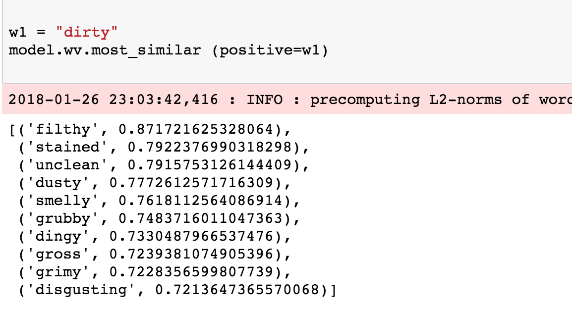
Let’s get to the fun stuff already! Since we trained on user reviews, it would be nice to see similarity on some adjectives. This first example shows a simple look up of words similar to the word ‘dirty’. All we need to do here is to call the most_similar function and provide the word ‘dirty’ as the positive example. This returns the top 10 similar words.
Ooh, that looks pretty good. Let’s look at more.
Similar to polite:
Similar to france:
Similar to shocked:
Overall, the results actually make sense. All of the related words tend to be used in similar contexts.
Now you could even use Word2Vec to compute similarity between two words in the vocabulary by invoking the similarity(...) function and passing in the relevant words.
Under the hood, the above three snippets compute the cosine similarity between the two specified words using word vectors (embeddings) of each. From the scores above, it makes sense that dirty is highly similar to smelly but dirty is dissimilar to clean. If you do a similarity between two identical words, the score will be 1.0 as the range of the cosine similarity can go from [-1 to 1] and sometimes bounded between [0,1] depending on how it’s being computed. You can read more about cosine similarity scoring here.
You will find more examples of how you could use Word2Vec in my Jupyter Notebook.
A closer look at the parameter settings
To train the model earlier, we had to set some parameters. Now, let’s try to understand what some of them mean. For reference, this is the command that we used to train the model.
model = gensim.models.Word2Vec(documents, size=150, window=10, min_count=2, workers=10, iter=10)size
The size of the dense vector to represent each token or word (i.e. the context or neighboring words). If you have limited data, then size should be a much smaller value since you would only have so many unique neighbors for a given word. If you have lots of data, it’s good to experiment with various sizes. A value of 100–150 has worked well for me for similarity lookups.
window
The maximum distance between the target word and its neighboring word. If your neighbor’s position is greater than the maximum window width to the left or the right, then, some neighbors would not be considered as being related to the target word. In theory, a smaller window should give you terms that are more related. Again, if your data is not sparse, then the window size should not matter too much, as long as it’s not overly narrow or overly broad. If you are not too sure about this, just use the default value.
min_count
Minimium frequency count of words. The model would ignore words that do not satisfy the min_count. Extremely infrequent words are usually unimportant, so its best to get rid of those. Unless your dataset is really tiny, this does not really affect the model in terms of your final results. The settings here probably has more of an effect on memory usage and storage requirements of the model files.
workers
How many threads to use behind the scenes?
iter
Number of iterations (epochs) over the corpus. 5 is a good starting point. I always use a minimum of 10 iterations.
Summing Up Word2Vec Tutorial
Now that you’ve completed this Gensim Word2Vec tutorial, think about how you’ll use it in practice. Imagine if you need to build a sentiment lexicon. Training a Word2Vec model on large amounts of user reviews helps you achieve that. You have a lexicon for not just sentiment, but for most words in the vocabulary.
Beyond raw unstructured text data, you could also use Word2Vec for more structured data. For example, if you had tags for a million stackoverflow questions and answers, you could find related tags and recommend those for exploration. You can do this by treating each set of co-occuring tags as a “sentence” and train a Word2Vec model on this data. Granted, you still need a large number of examples to make it work.
See Also: FastText vs. Word2Vec a Quick Comparison
Recommended Reading
- Fasttext vs. Word2Vec
- Introducing phrases in training a Word2Vec model (Phrase2Vec)
- Efficient Estimation of Word Representations in Vector Space
- Distributed Representations of Words and Phrases and their Compositionality
Resources
- Jupyter notebook for this tutorial
- Opinrank Original Dataset
I never got round to writing a tutorial on how to use word2vec in gensim. It’s simple enough and the API docs are straightforward, but I know some people prefer more verbose formats. Let this post be a tutorial and a reference example.
UPDATE: the complete HTTP server code for the interactive word2vec demo below is now open sourced on Github. For a high-performance similarity server for documents, see ScaleText.com.
Preparing the Input
Starting from the beginning, gensim’s word2vec expects a sequence of sentences as its input. Each sentence a list of words (utf8 strings):
# import modules & set up logging
import gensim, logging
logging.basicConfig(format='%(asctime)s : %(levelname)s : %(message)s', level=logging.INFO)

sentences = [['first', 'sentence'], ['second', 'sentence']]
# train word2vec on the two sentences
model = gensim.models.Word2Vec(sentences, min_count=1)
Keeping the input as a Python built-in list is convenient, but can use up a lot of RAM when the input is large.
Gensim only requires that the input must provide sentences sequentially, when iterated over. No need to keep everything in RAM: we can provide one sentence, process it, forget it, load another sentence…
For example, if our input is strewn across several files on disk, with one sentence per line, then instead of loading everything into an in-memory list, we can process the input file by file, line by line:
class MySentences(object):
    def __init__(self, dirname):
        self.dirname = dirname

    def __iter__(self):
        for fname in os.listdir(self.dirname):
            for line in open(os.path.join(self.dirname, fname)):
                yield line.split()

sentences = MySentences('/some/directory') # a memory-friendly iterator
model = gensim.models.Word2Vec(sentences)
Say we want to further preprocess the words from the files — convert to unicode, lowercase, remove numbers, extract named entities… All of this can be done inside the MySentences iterator and word2vec doesn’t need to know. All that is required is that the input yields one sentence (list of utf8 words) after another.
Note to advanced users: calling Word2Vec(sentences, iter=1) will run two passes over the sentences iterator (or, in general iter+1 passes; default iter=5). The first pass collects words and their frequencies to build an internal dictionary tree structure. The second and subsequent passes train the neural model. These two (or, iter+1) passes can also be initiated manually, in case your input stream is non-repeatable (you can only afford one pass), and you’re able to initialize the vocabulary some other way:
model = gensim.models.Word2Vec(iter=1)  # an empty model, no training yet
model.build_vocab(some_sentences)  # can be a non-repeatable, 1-pass generator
model.train(other_sentences)  # can be a non-repeatable, 1-pass generator
In case you’re confused about iterators, iterables and generators in Python, check out our tutorial on Data Streaming in Python.
Training
Word2vec accepts several parameters that affect both training speed and quality.
One of them is for pruning the internal dictionary. Words that appear only once or twice in a billion-word corpus are probably uninteresting typos and garbage. In addition, there’s not enough data to make any meaningful training on those words, so it’s best to ignore them:
model = Word2Vec(sentences, min_count=10) # default value is 5
A reasonable value for min_count is between 0-100, depending on the size of your dataset.
Another parameter is the size of the NN layers, which correspond to the “degrees” of freedom the training algorithm has:
model = Word2Vec(sentences, size=200) # default value is 100
Bigger size values require more training data, but can lead to better (more accurate) models. Reasonable values are in the tens to hundreds.
The last of the major parameters (full list here) is for training parallelization, to speed up training:
model = Word2Vec(sentences, workers=4) # default = 1 worker = no parallelization
The workers parameter has only effect if you have Cython installed. Without Cython, you’ll only be able to use one core because of the GIL (and word2vec training will be miserably slow).
Memory
At its core, word2vec model parameters are stored as matrices (NumPy arrays). Each array is #vocabulary (controlled by min_count parameter) times #size (size parameter) of floats (single precision aka 4 bytes).
Three such matrices are held in RAM (work is underway to reduce that number to two, or even one). So if your input contains 100,000 unique words, and you asked for layer size=200, the model will require approx. 100,000*200*4*3 bytes = ~229MB.
There’s a little extra memory needed for storing the vocabulary tree (100,000 words would take a few megabytes), but unless your words are extremely loooong strings, memory footprint will be dominated by the three matrices above.
Evaluating
Word2vec training is an unsupervised task, there’s no good way to objectively evaluate the result. Evaluation depends on your end application.
Google have released their testing set of about 20,000 syntactic and semantic test examples, following the “A is to B as C is to D” task: https://raw.githubusercontent.com/RaRe-Technologies/gensim/develop/gensim/test/test_data/questions-words.txt.
Gensim support the same evaluation set, in exactly the same format:
model.accuracy('/tmp/questions-words.txt')
2014-02-01 22:14:28,387 : INFO : family: 88.9% (304/342)
2014-02-01 22:29:24,006 : INFO : gram1-adjective-to-adverb: 32.4% (263/812)
2014-02-01 22:36:26,528 : INFO : gram2-opposite: 50.3% (191/380)
2014-02-01 23:00:52,406 : INFO : gram3-comparative: 91.7% (1222/1332)
2014-02-01 23:13:48,243 : INFO : gram4-superlative: 87.9% (617/702)
2014-02-01 23:29:52,268 : INFO : gram5-present-participle: 79.4% (691/870)
2014-02-01 23:57:04,965 : INFO : gram7-past-tense: 67.1% (995/1482)
2014-02-02 00:15:18,525 : INFO : gram8-plural: 89.6% (889/992)
2014-02-02 00:28:18,140 : INFO : gram9-plural-verbs: 68.7% (482/702)
2014-02-02 00:28:18,140 : INFO : total: 74.3% (5654/7614)
This accuracy takes an optional parameter restrict_vocab which limits which test examples are to be considered.
Once again, good performance on this test set doesn’t mean word2vec will work well in your application, or vice versa. It’s always best to evaluate directly on your intended task.
Storing and loading models
You can store/load models using the standard gensim methods:
model.save('/tmp/mymodel')
new_model = gensim.models.Word2Vec.load('/tmp/mymodel')
which uses pickle internally, optionally mmap‘ing the model’s internal large NumPy matrices into virtual memory directly from disk files, for inter-process memory sharing.
In addition, you can load models created by the original C tool, both using its text and binary formats:
model = Word2Vec.load_word2vec_format('/tmp/vectors.txt', binary=False)
# using gzipped/bz2 input works too, no need to unzip:
model = Word2Vec.load_word2vec_format('/tmp/vectors.bin.gz', binary=True)
Online training / Resuming training
Advanced users can load a model and continue training it with more sentences:
model = gensim.models.Word2Vec.load('/tmp/mymodel')
model.train(more_sentences)
You may need to tweak the total_words parameter to train(), depending on what learning rate decay you want to simulate.
Note that it’s not possible to resume training with models generated by the C tool, load_word2vec_format(). You can still use them for querying/similarity, but information vital for training (the vocab tree) is missing there.
Using the model
Word2vec supports several word similarity tasks out of the box:
model.most_similar(positive=['woman', 'king'], negative=['man'], topn=1)
[('queen', 0.50882536)]
model.doesnt_match("breakfast cereal dinner lunch";.split())
'cereal'
model.similarity('woman', 'man')
0.73723527
If you need the raw output vectors in your application, you can access these either on a word-by-word basis
model['computer']  # raw NumPy vector of a word
array([-0.00449447, -0.00310097,  0.02421786, ...], dtype=float32)
…or en-masse as a 2D NumPy matrix from model.syn0.
Bonus app
As before with finding similar articles in the English Wikipedia with Latent Semantic Analysis, here’s a bonus web app for those who managed to read this far. It uses the word2vec model trained by Google on the Google News dataset, on about 100 billion words:
The model contains 3,000,000 unique phrases built with layer size of 300.
Note that the similarities were trained on a news dataset, and that Google did very little preprocessing there. So the phrases are case sensitive: watch out! Especially with proper nouns.
On a related note, I noticed about half the queries people entered into the [email protected] demo contained typos/spelling errors, so they found nothing. Ouch.
To make it a little less challenging this time, I added phrase suggestions to the forms above. Start typing to see a list of valid phrases from the actual vocabulary of Google News’ word2vec model.
The “suggested” phrases are simply ten phrases starting from whatever bisect_left(all_model_phrases_alphabetically_sorted, prefix_you_typed_so_far) from Python’s built-in bisect module returns.
See the complete HTTP server code for this “bonus app” on github (using CherryPy).
Outro
Full word2vec API docs here; get gensim here. Original C toolkit and word2vec papers by Google here.
And here’s me talking about the optimizations behind word2vec at PyData Berlin 2014
Продолжаем решать NLP-задачи на примере корпуса с русскоязычными twitter-постами, на основе которого мы получили датасет [вот здесь]. Сегодня мы расскажем, как построить и обучить свою word2vec-модель Machine Learning, используя Python-библиотеку Gensim.
Модель Word2vec на основе датасета русскоязычных twitter-постов
В предыдущей статье мы подготовили датасет: провели лемматизацию и удалили стоп слова из корпуса, который содержит twitter-посты на русском языке [1]. Вот так он сейчас выглядят:
>>> data
0         [школотый, поверь, самый, общество, профилиров...
1          [да, таки, немного, похожий, но, мальчик, равно]
2                                 [ну, идиотка, испугаться]
3         [кто, угол, сидеть, погибать, голод, ещё, порц...
4         [вот, значит, страшилка, но, блин, посмотреть,...
...
205174                     [но, каждый, хотеть, исправлять]
205175          [скучать, вправлять, мозги, равно, скучать]
205176                       [вот, школа, говно, это, идти]
205177                           [тауриэль, грусть, обнять]
205178    [такси, везти, работа, раздумывать, приплатить...
Далее построим модель Word2vec, обученную на полученном датасете, с библиотекой Gensim [2].
Обучение модели Word2vec
Подготовив датасет, можем обучить модель. Для этого воспользуемся библиотекой Gensim и инициализируем модель Word2vec:
from gensim.models import Word2Vec

w2v_model = Word2Vec(
    min_count=10,
    window=2,
    size=300,
    negative=10,
    alpha=0.03,
    min_alpha=0.0007,
    sample=6e-5,
    sg=1)
Модель имеет множество аргументов:
min_count— игнорировать все слова с частотой встречаемости меньше, чем это значение.windоw— размер контекстного окна, о котором говорили тут, обозначает диапазон контекста.size— размер векторного представления слова (word embedding).negative— сколько неконтекстных слов учитывать в обучении, используя negative sampling, о нем также упоминалось здесь.alpha— начальный learning_rate, используемый в алгоритме обратного распространения ошибки (Backpropogation).min_alpha— минимальное значение learning_rate, на которое может опуститься в процессе обучения.sg— если 1, то используется реализация Skip-gram; если 0, то CBOW. О реализациях также говорили тут.
Далее, требуется получить словарь:
w2v_model.build_vocab(data)
А после уже можно обучить модель, используя метод train:
w2v_model.train(data, total_examples=w2v_model.corpus_count, epochs=30, report_delay=1)
Если в дальнейшем не требуется снова обучать модель, то для сохранения оперативной памяти можно написать следующее:
w2v_model.init_sims(replace=True)
Насколько похожи слова обученной модели Word2vec
После того, как модель была обучена, можем смотреть результаты. Каждое слово представляется вектором, следовательно, их можно сравнивать. В качестве инструмента сравнения в Gensim используется косинусный коэффициент (Cosine similarity) [3].
У модели Word2vec имеется в качестве атрибута объект wv, который и содержит векторное представление слов (word embeddings). У этого объекта есть методы для получения мер схожестей слов. Например, определим, какие слова находятся ближе всего к слову “любить”:
>>> w2v_model.wv.most_similar(positive=["любить"])
[('дорожить', 0.5577003359794617),
('скучать', 0.4815309941768646),
('обожать', 0.477267324924469),
('машенька', 0.4503161907196045),
('предновогодниеобнимашка', 0.4403109550476074),
('викуль', 0.43941542506217957),]
Число после запятой обозначает косинусный коэффициент, чем он больше, тем выше близость слов. Можно заметить, что слова “дорожить”, “скучать”, “обожать” наиболее близкие к слову “любить” Можно также рассмотреть другие слова:
>>> w2v_model.wv.most_similar(positive=["мужчина"])
[('женщина', 0.6242121458053589),
('девушка', 0.5410279035568237),
('любящий', 0.5005632638931274),
('парень', 0.4864271283149719),
('идеал', 0.45188209414482117),
('существо', 0.44532185792922974),
('недостаток', 0.4350862503051758),
('пёсик', 0.42453521490097046),
('послушный', 0.42428380250930786),
('эгоизм', 0.4202057421207428)]
...
>>> w2v_model.wv.most_similar(positive=["день", "завтра"])
[('сегодня', 0.6082668304443359),
('неделя', 0.5371285676956177),
('суббота', 0.48631012439727783),
('выходной', 0.4772387742996216),
('понедельник', 0.4697558283805847),
('денёчек', 0.4688040316104889),
('каникулы', 0.45828908681869507),
('подъесть', 0.4555707573890686),
('отсыпаться', 0.44570696353912354),
('аттестация', 0.4408838450908661)]
Векторы можно складывать и вычитать. Например, рассмотрим такой вариант: “папа” + “брат” — “мама”. Получили следующее:
>>> w2v_model.wv.most_similar(positive=["папа", "брат"], negative=["мама"])
[('младший', 0.3892076015472412),
('сестра', 0.31560415029525757),
('двоюродный', 0.3024488091468811),
('старший', 0.2937452793121338),]
Как видим, на этом корпусе результатом являются слова “младший”, “сестра”, “двоюродный”. Несмотря на то, что мы обучили модель на twitter-постах, получаем достаточно адекватные результаты.
Есть также возможность определить наиболее близкое слово из списка к данному слово. Для этого нужно воспользоваться методом:
>>> w2v_model.wv.most_similar_to_given("хороший", ["приятно", "город", "мальчик"])
'приятно'
Слово “приятно” из всего списка наиболее близок к слову “хороший”. Кроме того, так как для сравнения находится косинусный коэффициент, то его можно получить, написав:
>>> w2v_model.wv.similarity("плохой", "хороший")
0.5427995
>>> w2v_model.wv.similarity("плохой", "герой")
0.04865976
Само векторное представление слова можно получит либо напрямую, обратившись через квадратные скобки, либо через метод word_vec:
>>> w2v_model.wv.word_vec("страшилка")
array([-0.05101333, -0.03730767,  0.03676478,  0.18950877,  0.02496774,
        0.00176699, -0.0966768 ,  0.04010197, -0.00862965, -0.00530563,
...
dtype=float32)
>>> w2v_model.wv["страшилка"]
array([-0.05101333, -0.03730767,  0.03676478,  0.18950877,  0.02496774,
        0.00176699, -0.0966768 ,  0.04010197, -0.00862965, -0.00530563,
...
dtype=float32)
>>> w2v_model.wv.word_vec("страшилка").shape
(300,)
Векторное представление слов на плоскости
Так как слова в модели Word2vec — это векторы, то можно их выстроить на координатную плоскость. Поскольку каждый вектор модели имеет размерность 300, который был указан как аргумент size, то не предоставляется возможности построить 300-мерное пространство. Поэтому мы воспользуемся методом уменьшения размерности t-SNE, который есть в Python-библиотеке Scikit-learn [4], и снизим размерность векторов с 300 до 2. Согласно документации, если размерность больше 50, то стоит сначала воспользоваться другим методом уменьшения размерности — методом главных компонент PCA [5]. Для этого в аргументе достаточно указать init=”pca”.
В результате мы написали функцию, которая принимает входное слово и список слов и строит на плоскости входное слово, ближайшие к нему слова и переданный список слов:
import matplotlib.pyplot as plt
import seaborn as sns
from sklearn.manifold import TSNE

def tsne_scatterplot(model, word, list_names):
    """Plot in seaborn the results from the t-SNE dimensionality reduction
    algorithm of the vectors of a query word,
    its list of most similar words, and a list of words."""
    vectors_words = [model.wv.word_vec(word)]
    word_labels = [word]
    color_list = ['red']

    close_words = model.wv.most_similar(word)
    for wrd_score in close_words:
        wrd_vector = model.wv.word_vec(wrd_score[0])
        vectors_words.append(wrd_vector)
        word_labels.append(wrd_score[0])
        color_list.append('blue')

    # adds the vector for each of the words from list_names to the array
    for wrd in list_names:
        wrd_vector = model.wv.word_vec(wrd)
        vectors_words.append(wrd_vector)
        word_labels.append(wrd)
        color_list.append('green')

    # t-SNE reduction
    Y = (TSNE(n_components=2, random_state=0, perplexity=15, init="pca")
        .fit_transform(vectors_words))
    # Sets everything up to plot
    df = pd.DataFrame({"x": [x for x in Y[:, 0]],
                    "y": [y for y in Y[:, 1]],
                    "words": word_labels,
                    "color": color_list})
    fig, _ = plt.subplots()
    fig.set_size_inches(9, 9)
    # Basic plot
    p1 = sns.regplot(data=df,
                    x="x",
                    y="y",
                    fit_reg=False,
                    marker="o",
                    scatter_kws={"s": 40,
                                "facecolors": df["color"]}
    )
    # Adds annotations one by one with a loop
    for line in range(0, df.shape[0]):
        p1.text(df["x"][line],
                df["y"][line],
                " " + df["words"][line].title(),
                horizontalalignment="left",
                verticalalignment="bottom", size="medium",
                color=df["color"][line],
                weight="normal"
        ).set_size(15)

    plt.xlim(Y[:, 0].min()-50, Y[:, 0].max()+50)
    plt.ylim(Y[:, 1].min()-50, Y[:, 1].max()+50)
    plt.title('t-SNE visualization for {}'.format(word.title()))
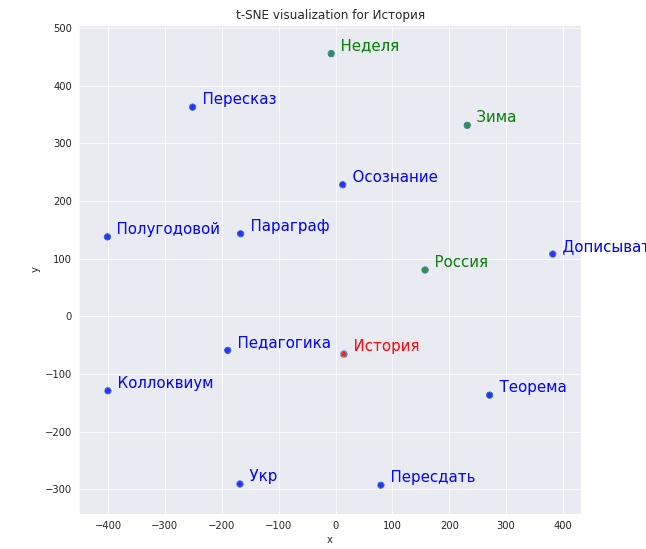
Далее рассмотрим, как далеко располагается слово “история” и слова «неделя», «россия», «зима»:
tsne_scatterplot(w2v_model, "история", ["неделя", "россия", "зима"])
Рисунок ниже показывает результат уменьшения размерности. Как видим, около истории находятся слова, связанные с учебой (“педагогика”, “теорема”), а вот “неделя”, которую мы передали как элемент списка, находится далеко от “истории”.
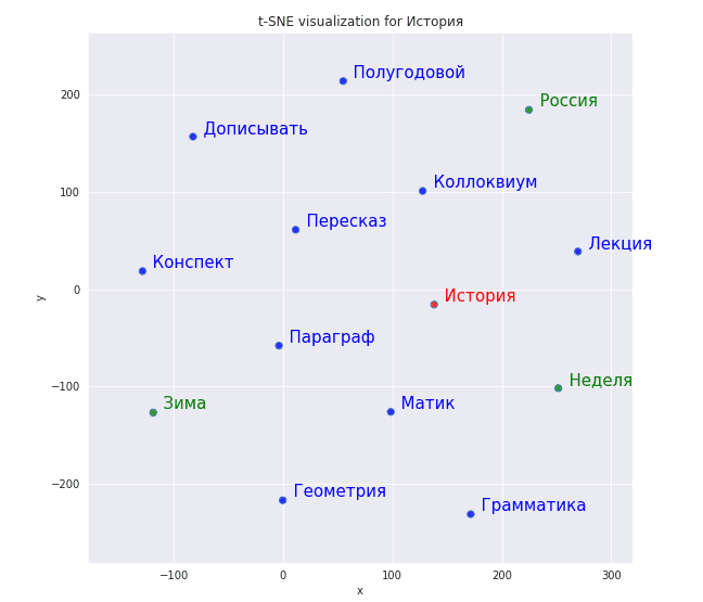
Мы переобучили модель, увеличив число эпох обучения (аргумент epoch в методе train) в два раза, и построили через ту же самую функцию систему координат:
Результаты оправдали себя, с “историей” стало ассоциироваться больше слов, связанных с учебой и приблизилась к нему “неделя”. Machine Learning требует постоянного экспериментирования, поэтому важно всячески настраивать и перенастраивать свою модель.
Еще больше подробностей о NLP-моделях и особенностях их обучения на реальных примерах Data Science с помощью средств языка Python, вы узнаете на наших курсах в лицензированном учебном центре обучения и повышения квалификации ИТ-специалистов в Москве.
Источники
- Рубцова Ю. Автоматическое построение и анализ корпуса коротких текстов (постов микроблогов) для задачи разработки и тренировки тонового классификатора //Инженерия знаний и технологии семантического веба. – 2012. – Т. 1. – С. 109-116.
- https://radimrehurek.com/gensim/
- https://en.wikipedia.org/wiki/Cosine_similarity
- https://scikit-learn.org/stable/modules/generated/sklearn.manifold.TSNE.html
- https://ru.wikipedia.org/wiki/Метод_главных_компонент


