
The following is a list of stop words that are frequently used in english language.
Where these stops words normally include prepositions, particles, interjections, unions, adverbs, pronouns, introductory words, numbers from 0 to 9 (unambiguous), other frequently used official, independent parts of speech, symbols, punctuation. Relatively recently, this list was supplemented by such commonly used on the Internet sequences of symbols as www, com, http, etc.
There are 2 views of stop words for english language: table and list. Just use the view which is the most convenient to you.
For the external usage, you can always download stop words for english as XML, TXT or JSON formats.
Время на прочтение
11 мин
Количество просмотров 12K

Автор статьи — Виктория Ляликова.
В данной статье хотелось бы рассказать о том, как можно применить различные методы машинного обучения (ML) для обработки текста, чтобы можно было произвести его бинарную классифицию.
Рассмотрим задачу обработки естественного языка (NLP — Natural Lanuage Processing) на примере классификации психического здоровья для определения депрессии по комментариям в Reddit. Посмотрим на наш датасет:
import pandas as pd
data_depression = pd.read_csv('D:/vika/datasets/depression_dataset_reddit_cleaned.csv')
data_depression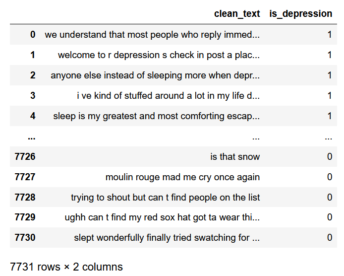
Посмотрим, например, на какую-нибудь одну запись:
‘sleep is my greatest and most comforting escape whenever i wake up these day the literal very first emotion i feel is just misery and reminding myself of all my problem i can t even have a single second to myself it s like waking up everyday is just welcoming yourself back to hell’.
Данный комментарий классифицируется как наличие депрессии у человека.
Далее посмотрим на гистограмму распределения.
import seaborn as sns
sns.countplot(data=data_depression, x="is_depression")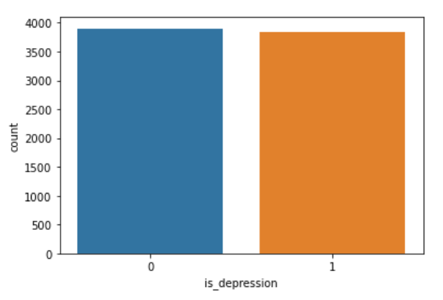
То есть можно увидеть, что в датасете количество комментариев соответствующих депрессии и ее отсутствию распределено приблизительно одинаково.Теперь приступим к обработке текста, чтобы его можно было применять в алгоритмах машинного обучения.
Сначала необходимо импортировать библиотеку NLTK, которая является ведущей для создания программ по обработке естественного языка на Python. И рассмотрим основные методы данного инструмента.
Также нам понадобится загрузить модуль RE, который является модулем по работе с регулярными выражениями и также помогает работать с текстом. Данный модуль позволяет производить поиск, замену, анализ и другие операции по работе с текстом.
import nltk
import re

nltk.download("stopwords") # поддерживает удаление стоп-слов
nltk.download('punkt') # делит текст на список предложений
nltk.download('wordnet') # проводит лемматизацию
from nltk.corpus import stopwords
Рассмотрим основные шаги, которые необходимы для обработки текста.
-
Очистка текста от неалфавитных символов. Функция
re.subпозволяет заменить все, что подходит под шаблон на указанную строку. Например, вот так можно заменить все, что не является словами на пробелы:
re.sub("[^a-zA-Z]"," ",text)-
Токенизация. Данный метод позволяет разделить текст на так называемые токены, то есть на слова или предложения.
nltk.word_tokenize(text,language = "english")-
Лемматизация. Позволяет привести словоформу к лемме — ее нормальной (словарной) форме. Другими словами, лемматизация схожа с выделением основы каждого слова в предложении. Она обычно выполняется простым поиском форм в таблице. Кроме того, можно добавить некоторые пользовательские правила для анализа слов.
lemmatize = nltk.WordNetLemmatizer()
lemmatize.lemmatize(word) for word in text-
Удаление стоп-слов. Под стоп-словами обычно понимаются артикли, междометия, союзы и т.д., которые не несут смысловой нагрузки. При применении алгоритмов машинного обучения такие слова могут добавить много шума, поэтому лучше избавляться от них. В NLTK есть предустановленный список стоп-слов.
lemmatize.lemmatize(word) for word in text if not word in set(stopwords.words("stopwords"))-
Векторизация текста или преобразование текста в численную форму. Алгоритмы машинного обучения не умеют работать с текстом, поэтому необходимо превратить текст в цифры. Данная стратегия называется представлением «Мешок слов». Документы описываются вхождениями слов, при этом полностью игнорируется информация об относительном положении слов в документе. По мешку слов находят количество появлений каждого слова во всем тексте.
В пакете scikit-learn есть модуль CountVectorizer, который преобразовывает входной текст в матрицу, значениями которой являются количества вхождения данного ключа(слова) в текст. Таким образом, мы получим матрицу, размерность которой будет равна количеству всех слов, умноженных на количество документов. И элементами матрицы будут числа, которые означают, сколько раз всего слово встретилось в тексте.

Также популярным методом для векторизации текста является метод TF-IDF, который является статистической мерой для оценки важности слова в документе.
В тексте большого объема некоторые слова могут присутствовать очень часто, но при этом не нести никакой значимой информации о фактическом содержании текста (документа). Если такие данные передавать непосредственно классификатору, то такие частые термины могут затенять частоты более редких, но при этом более интересных терминов. Для того, чтобы этого избежать, достаточно разделить количество употреблений каждого слова в документе на общее количество слов в документе, это есть TF — частота термина. Термин IDF (inverse document frequency) обозначает обратную частоту термина (инверсия частоты) с которой некоторое слово встречается в документах. IDF позволяет измерить непосредственную важность термина.
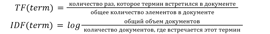
Тогда TF-IDF вычисляется следующим образом:
TF-IDF(term)=TF(term)*IDF(term)

В итоге код по работе с текстом выглядит следующим образом,
new_text = []
for i in data_depression.clean_text:
    #удаляем неалфавитные символы
    text = re.sub("[^a-zA-Z]"," ",i)
    # токенизируем слова
    text = nltk.word_tokenize(text,language = "english")
    # лемматирзируем слова
    text = [lemmatize.lemmatize(word) for word in i]
    # соединяем слова
    text = "".join(text)
    new_text.append(text)
В данной задаче текст будем преобразовывать в набор цифр с помощью модуля CountVectorizer для получения матрицы, содержащей 0 и 1.
# импортируем модуль
from sklearn.feature_extraction.text import CountVectorizer
count = CountVectorizer(stop_words="english")
# проводим преобразование текста
matrix = count.fit_transform(new_text).toarray()
Если мы ходим преобразовать текст, используя метод TF-IDF, тогда можно поступить следующим образом:
# импортируем модуль TfidfVectorizer
from sklearn.feature_extraction.text import TfidfVectorizer
tfidf_vectorizer = TfidfVectorizer(stop_words="english")
#преобразуем текст
values = tfidf_vectorizer.fit_transform(new_text)
После того, как обработка текста закончена, можно переходить непосредственно к применению алгоритмов машинного обучения.
Определим вектор с данными для обучения и вектор правильных ответов.
X=matrix
y = data_depression["is_depression"].values
Далее разделим выборку на тестовую и обучающую
from sklearn.model_selection import train_test_split
x_train, x_test, y_train, y_test = train_test_split(X, y, test_size = 0.33, random_state = 42)
Рассмотрим самый известный алгоритм — наивный классификатор Байеса. Данный алгоритм является одним из самых простых алгоритмов классификации, но при этом часто может работать не хуже более сложных алгоритмов. Метрики качества работы алгоритмов будут приведено ниже. Пока буду приводить только точность алгоритмов.
from sklearn.naive_bayes import GaussianNB
nb = GaussianNB()
result_bayes = nb.fit(x_train, y_train)
nb.score(x_test,y_test)
0.8436520376175548
Логистическая регрессия. Также является простейшим алгоритмом классификации. С помощью данного алгоритма можно разделить несложные объекты на 2 класса. Модель логистической регрессии быстро обучается и подходит для задач бинарной классификации.
from sklearn.linear_model import LogisticRegression
logreg = LogisticRegression()
result_logreg = logreg.fit(x_train, y_train)
logreg.score(x_test,y_test)
0.9564655172413793
Метод опорных векторов. Данный метод также можно использовать для задач классификации, поскольку он категоризирует данные с помощью гиперплоскости.
from sklearn import svm
metodsvm = svm.SVC()
result_svm = metodsvm.fit(x_train, y_train)
metodsvm.score(x_test, y_test)
0.9543103448275863
Теперь можно попробовать рассмотреть некоторые ансамблевые методы машинного обучения, такие как адаптивный бустинг и градиентный бустинг. Что мы знаем про ансамблевые методы? В ансамблевых методах несколько моделей обучаются для решения одной и той же проблемы и объединяются для получения более эффективных результатов. Основная идея заключается в том, что при правильном сочетании моделей можно получить более точную и надежную модель.
Считается, что алгоритм адаптивного бустинга лучше всего работает со слабыми обучающими алгоритмами и может достичь достаточно высокой точности при решении задач классификации. В AdaBoost базовые алгоритмы обучаются последовательно, учитывая опыт предыдущего. Так, каждый последующий алгоритм начинает придавать большее значение тем наблюдениям из тренировочного набора данных, на которых ошиблись предыдущие.
#адаптивный бустинг

from sklearn.tree import DecisionTreeClassifier
from sklearn.model_selection import train_test_split
from sklearn.ensemble import AdaBoostClassifier

modelClf = AdaBoostClassifier(base_estimator=DecisionTreeClassifier(max_depth=2), n_estimators=100, random_state=42)

X_train, X_valid, y_train, y_valid = train_test_split(X, y, test_size = 0.33, random_state = 42)

modelclf_fit = modelClf.fit(X_train, y_train)
modelClf.score(X_valid, y_valid)
0.9361285266457681
Градиентный бустинг, также как и адаптивный, обучает слабые алгоритмы последовательно, исправляя ошибки предыдущих. Принципиальное отличие этих алгоритмов заключается в способах изменения весов. Адаптивный бустинг использует итеративный метод оптимизации, в то время как градиентный оптимизирует веса с помощью градиентного спуска.
# градиентный бустинг

from sklearn.model_selection import train_test_split
# импортируем библиотеку
from sklearn.ensemble import GradientBoostingClassifier

modelClf = GradientBoostingClassifier(max_depth=2, n_estimators=150,random_state=12, learning_rate=1)

X_train, X_valid, y_train, y_valid = train_test_split(X, y,
                                                      test_size=0.3, random_state=12)

modelClf.fit(X_train, y_train)
modelClf.score(X_valid, y_valid)
0.928448275862069
И напоследок хочется рассмотреть алгоритм работы простой нейронной сети (многослойный персептрон), в которой будет 2 полносвязнных слоя и 1 выходной с 1 выходом. Чтобы смоделировать нейронную сеть в python, нам понадобится фреймворк Keras, который является оболочкой над Tensorflow.
В Keras для построения моделей нейронных сетей (models) мы собираем слои (layers). Для описания стандартных архитектур нейронных сетей в Keras уже существуют предопределенные классы для слоев:
-
Dense() – полносвязный слой;
-
Conv1D, Conv2D, Conv3D – сверточные слои;
-
Conv2DTranspose, Conv3DTranspose – транспонированные (обратные) сверточные слои;
-
SimpleRNN, LSTM, GRU – рекуррентные слои;
-
MaxPooling2D, Dropout, BatchNormalization – вспомогательные слои
Обратим внимание, что в Keras слои автоматически конструируются таким образом, чтобы соответствовать форме входного слоя, поэтому нет необходимости беспокоиться о совместимости слоев, что очень удобно.
Типичный процесс использования Keras для построения нейронной сети можно описать так:
-
Определение обучающих данных: входные и целевые векторы
-
Определение слоев сети (модель), отображающих входные данные в целевые
-
Настройка процесса обучения выбором функции потерь, оптимизатора и некоторых параметров для мониторинга
-
Выполнение итераций по обучающим данным вызовом метода
fit()и модели.
Если мы хотим создать нейронную сеть с последовательными слоями, нам также понадобится класс Sequential.
Загружаем необходимые библиотеки:
from keras import models
from keras import layers
from tensorflow.keras.models import Sequential
from tensorflow.keras.layers import Dense1. Получаем обучающую и тестовую выборку:
x_train, x_test, y_train, y_test = train_test_split(X, y, test_size = 0.33, random_state = 42)2. Сначала создаем пустую модель Sequential:
model = models.Sequential()Теперь в пустую модель нейронной сети можно добавлять слои. Добавим 2 полносвязных слоя с 64 выходными нейронами и активационной функцией Relu (фактор нелинейности). Функция relu является самой популярной функцией в глубоком обучении, но, конечно, можно использовать и другие. Первому слою надо обязательно передать ожидаемую форму входных данных, т.е. размер входного вектора, это указывается в параметре input_shape.
model.add(layers.Dense(64,activation='relu',input_shape=(voc_len,)))
model.add(layers.Dense(64, activation='relu'))
model.add(layers.Dense(1, activation = 'sigmoid'))
Последний слой сети имеет сигмоидальную активационную функцию, так как наша задача является задачей бинарной классификации и на выходе сети мы хотим получить оценку вероятности между 0 и 1 того, что наш образец относится к классу “1”.
3. После того, как модель создана, необходимо настроить процесс ее обучения с помощью вызова метода compile
from keras import optimizers
model.compile(optimizer='rmsprop',loss='binary_crossentropy',metrics=['accuracy'])
Объект optimizer определяет процедуру обучения, а именно оптимизатор алгоритма градиентного спуска. Доступны оптимизаторы SGD, RMSprop, Adam, Adadelta, Adagrad, Adamax, Nadam, Ftrl.
Объект loss — это функция, которая минимизируется в процессе обучения. Среди распространенных вариантов: среднеквадратичная ошибка (mse), categorical_crossentropy, binary_crossentropy.
Объект metrics используется для мониторинга обучения.
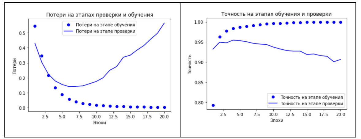
4. Для обучения модели необходимо вызвать метод fit(). Задаем тренировочные данные, количество эпох для обучения, валидационные данные для отслеживания производительности модели, что позволит отобразить значения функции потерь и метрики в режиме вывода для передаваемых данных в конце каждой эпохи. Зададим 20 эпох, чтобы потом можно было найти оптимальное количество эпох, которое необходимо для обучения.
history=model.fit(x_train, y_train, epochs=20,batch_size=512,validation_data=(x_test,y_test))Вызов метода fit вернет нам объект history, с помощью которого можно получить данные обо всем происходящем в процессе обучения.
history_dict = history.history
history_dict.keys()
dict_keys(['loss', 'accuracy', 'val_loss', 'val_accuracy'])
Теперь можно вывести графики потерь и точности на этапах обучения и проверки
# построение графика потери на этапах проверки и обучения
loss_values = history_dict['loss']
val_loss_values = history_dict['val_loss']
epochs = range(1, len(history_dict['accuracy'])+1)

# построение графика потери на этапах проверки и обучения
loss_values = history_dict['loss']
val_loss_values = history_dict['val_loss']
epochs = range(1, len(history_dict['accuracy'])+1)

plt.plot(epochs, loss_values, 'bo', label = 'Потери на этапе обучения')
plt.plot(epochs, val_loss_values, 'b', label = 'Потери на этапе проверки')
plt.title('Потери на этапах обучения и проверки')
plt.xlabel('Эпохи')
plt.ylabel('Потери')
plt.legend()
plt.show()

# построение графика точности на этапах обучения и проверки
acc_values = history_dict['accuracy']
val_acc_values = history_dict['val_accuracy']
plt.plot(epochs, acc_values, 'bo', label = 'Точность на этапе обучения')
plt.plot(epochs, val_acc_values, 'b', label = 'Точность на этапе проверки')
plt.title('Точность на этапах обучения и проверки')
plt.xlabel('Эпохи')
plt.ylabel('Точность')
plt.legend()
plt.show()
Посмотрев на графики, можно увидеть, что на этапе обучения потери снижаются с каждой эпохой, а точность растет. Как раз такого поведения и можно ожидать от оптимизации градиентным спуском, та величина, которую мы минимизируем, должна становиться все меньше с каждой итерацией. Но это не относится к потерям и точности на этапе проверки, можно заметить, что здесь пик был достигнут где-то на 4-5 эпохе. И, начиная с пятой эпохи, наблюдается переобучение, которое выражается в том, что функция потерь начинает расти. Такой картины стоило ожидать, так как модель, которая показывает хорошие результаты на обучающих данных, не обязательно будет показывать такие же хорошие результаты на данных, которых никогда не видела.
Благодаря такому графику можно оценить оптимальное количество эпох, которое необходимо для обучения сети. В данном случае для предотвращения переобучения нейронную сеть будем обучать на 5 эпохах. Таким образом, обучим сеть с нуля и рассчитаем метрики качества разработанной модели нейронной сети.
Y_pred=model.predict(x_test)
# задаем порог 0,5 для классификации текста
Y_pred=(Y_pred>=0.5).astype("int")
from sklearn.metrics import confusion_matrix
from sklearn.metrics import classification_report
print(classification_report(y_test,Y_pred))
print(confusion_matrix(y_test,Y_pred))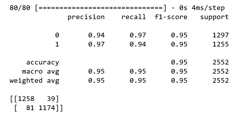
Результаты работы всех алгоритмов можно увидеть в таблице
|
Алгоритм |
Accuracy |
Precision |
Recall |
F1 |
|
Классификатор Байеса |
0.844 |
0.785 |
0.939 |
0.855 |
|
Логистическая регрессия |
0.956 |
0.987 |
0.924 |
0.954 |
|
Метод опорных векторов |
0.954 |
0.998 |
0.909 |
0.951 |
|
AdaBoost |
0.936 |
0.935 |
0.935 |
0.935 |
|
GradientBoost |
0.928 |
0.953 |
0.896 |
0.924 |
|
Многослойный персептрон |
0.953 |
0.968 |
0.937 |
0.951 |
Посмотрев на данную сравнительную таблицу, можно сказать, что классификатор Байеса, к сожалению, показал самые плохие результаты с точностью 0,84. У алгоритма адаптивного бустинга одинаковые показатели по всем метрикам, равные 0.94. Это связано с тем, что целью данного алгоритма является улучшение производительности алгоритмов. На мой взгляд, можно выделить 3 алгоритма, которые хорошо справились с задачей — это логистическая регрессия, метод опорных векторов и многослойный персептрон с точностью 0,95.
Приглашаем на открытое занятие «Пишем первую нейронную сеть». На нем рассмотрим основные этапы создания и обучения своей первой нейронной сети и попробуем решить известную задачу классификации MNIST полносвязной и сверточной нейронными сетями на примере фреймворка PyTorch. Регистрация — по ссылке.
Я описал инструменты и методы для новичков, имеющих только общее представление в данной теме. Если вы более опытный практик, вам нужны вторая часть о представлении вектора и третья — тематическое моделирование и конвейеры. Конечно, в этой области есть свой жаргон. Он может немного напугать, но я сведу технические термины к минимуму.
Вам понадобится базовое понимание Python и какой-то опыт в машинном обучении желателен, но не обязателен. Как всегда, я даю ссылки на документацию там, где в объяснениях или приёмах не останавливаюсь на деталях.
Токенизация
Токен — это последовательность символов в документе, имеющая значение для анализа. Обычно это отдельные слова, но не всегда. Документ — это коллекция текста. Им может быть твит, книга или что-то еще. Признаки хороших токенов:
- Хранятся в перечисляемых структурах (список, генератор) для упрощения анализа в будущем.
- Имеют единый регистр для одной цели.
- Содержат только буквы и цифры.
Пример: токенизация
import re

def tokenize(text):

    text = text.lower()

    text = re.sub(r'[^a-zA-Z ^0-9]', '', str(text))

    return text.split()

# Используем оригинал текста выше

tokens = tokenize(sample_text)

tokens[:10]

____________________________________________________________________

['a',  'token',  'is',  'a',  'sequence',  'of',  'characters',  'in',  'a',  'document']
Подсчёт слов
Теперь, когда у нас есть токены, мы можем приступить к самому простому анализу. Подсчитаем количество слов через Counter.
from collections import Counter

def word_counter(tokens):

    word_counts = Counter()

    word_counts.update(tokens)

    return word_countsword_count =

word_counter(tokens)

word_count.most_common(5)

____________________________________________________________________

[('a', 7), ('of', 4), ('in', 4), ('be', 4), ('an', 3)]
И отобразим на гистограмме:
import matplotlib.pyplot as plt

x = list(word_count.keys())[:10]

y = list(word_count.values())[:10]

plt.bar(x, y)

plt.show();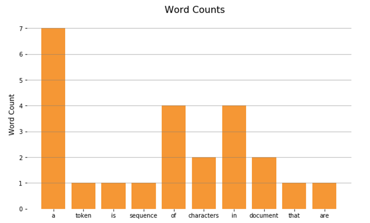
3. Состав документа
Количество слов может быть полезно, но обычно требуется более глубокий анализ, отвечающий на вопросы бизнеса, особенно когда данные состоят не из одного документа. Мы можем настроить себя на успех, создав Pandas DataFrame, содержащий функции, возвращающие:
- Количество и процент документов с токеном.
- Количество токенов.
- Их ранг по частотности употребления по отношению к другим токенам.
- Процент токенов от общего состава документа.
- Текущую сумму этих процентов.
Пример: анализ состава документов с DataFrame
import pandas as pddef count(docs):
word_counts = Counter()
appears_in = Counter()
total_docs = len(docs)
for doc in docs:
word_counts.update(doc)
appears_in.update(set(doc))
temp = list(zip(word_counts.keys(), word_counts.values()))
# Колонки слов и количества
wc = pd.DataFrame(temp, columns = ['word', 'count'])
# Колонка ранга
wc['rank'] = wc['count'].rank(method='first', ascending=False)
# Колонка с общим процентом
total = wc['count'].sum()
wc['pct_total'] = wc['count'].apply(lambda x: x / total)
# Колонка с кумулятивным общим процентом
wc = wc.sort_values(by='rank')
wc['cul_pct_total'] = wc['pct_total'].cumsum()
# Появляется в колонке
t2 = list(zip(appears_in.keys(), appears_in.values()))
ac = pd.DataFrame(t2, columns=['word', 'appears_in'])
wc = ac.merge(wc, on='word')
# Появляется в колонке процентов
wc['appears_in_pct'] = wc['appears_in'].apply(lambda x: x / total_docs)
return wc.sort_values(by='rank')
wc = count([tokens])wc.head()
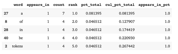
С помощью DataFrame мы видим график функции распределения вероятностей, показывающий, как ранг токена связан с совокупным составом наших документов:
import seaborn as sns

sns.lineplot(x = 'rank', y = 'cul_pct_total', data = wc)

plt.show();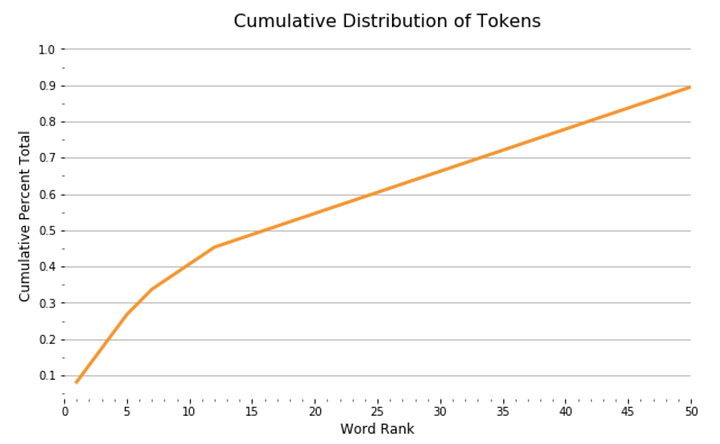
Из графика видно, что 13 наиболее употребимых токенов составляют 45% документа, а после распределение выглядит довольно равномерным. Мы можем увидеть относительный процент этих токенов в составе документа в виде сплошных занимаемых ими участков документа:
import squarify

wc_top13 = wc[wc['rank'] <= 13]

squarify.plot(sizes=wc_top13['pct_total'], label=wc_top13['word'], alpha=.8 )

plt.axis('off')

plt.show();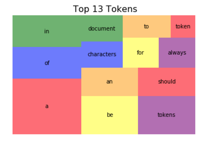
Эти примеры демонстрируют принципы, необходимые для более глубокого понимания мира обработки естественного языка. Токенизация, подсчёт слов и анализ состава документов — основополагающие концепции. Мы могли бы написать целую библиотеку с нуля, но обычно это не самый эффективный способ решения проблем. Существует зоопарк библиотек с открытым кодом, но только одна из них — лидер в области.
4. Введение в SpaCy
SpaСy — свободная, открытая библиотека Python для решения передовых задач NLP, разработанная Explosion. Она не хранит повторяющиеся компоненты документов в разных структурах данных. Вместо этого SpaСy индексирует компоненты и хранит уточняющую информацию. Поэтому её считают эффективнее в проектах производственного класса, чем библиотеки вроде NLTK. Токены в SpaCy:
import spacy

nlp = spacy.load("en_core_web_lg")

def spacy_tokenize(text):

    doc = nlp.tokenizer(text)

    return [token.text for token in doc]

spacy_tokens = spacy_tokenize(sample_text)

spacy_tokens[:10]

____________________________________________________________________

['a',  'token',  'is',  'a',  'sequence',  'of',  'characters',  'in',  'a',  'document']
5. Стоп-слова
Слова “I”, “and”, “of” и тому подобные почти не имеют смысловой нагрузки. Мы называем их стоп-словами и в анализ не включаем. Большинство библиотек имеют встроенный список часто используемых английских слов. Союзов, артиклей, наречий, предлогов и общеупотребимых глаголов. Однако лучшая практика — настройка списка под задачу.
Пример удаления стоп-слов:
spacy_stopwords = spacy.lang.en.stop_words.STOP_WORDS
def remove_stopwords(tokens):
cleaned_tokens = []
for token in tokens:
if token not in spacy_stopwords:
cleaned_tokens.append(token)
return cleaned_tokens
cleaned_tokens = remove_stopwords(spacy_tokens)
cleaned_tokens[:10]
____________________________________________________________________
['A', 'token', 'sequence', 'characters', 'document', 'useful', 'analytical', 'purpose', '.', 'Often']
6. Леммы
Лемматизация — поиск леммы слова или корневого слова. Говоря простым языком, лемма — это то слово, которое можно найти в словаре. Например, бег, бежит, бегущий, бежал — формы одной и той же лексемы (слова) с леммой “бег”. Пример лемматизации:
def spacy_lemmatize(text):

    doc = nlp.tokenizer(text)

    return [token.lemma_ for token in doc]

spacy_lemmas = spacy_lemmatize(sample_text)

spacy_lemmas[:10]

____________________________________________________________________

['A', 'token', 'be', 'a', 'sequence', 'of', 'character', 'in', 'a', 'document']
Заключение
Токены, состав документа, стоп-слова, леммы — все они играют свою роль в обработке естественного языка, хотя они довольно просты сами по себе. Мой следующий пост NLP в Python: представления вектора погрузит нас глубже в тему NLP.
Jupyter Notebook на Github
I was wondering if anyone could help me with the following problem:
I am trying to determine the number (count) of stop words in customer review texts. I am using the «quanteda» package stop words list in R.
I have tokenised the text and filtered out the stop words by using the following code:
stop.words <- tokens_select(corpus2.tokens, stopwords())
However, I am now having trouble saving these results in such a way that I can count the actual number of stopwords included in each review.
Any tipps would be greatly appreciated. Thanks in advance!
asked Apr 21, 2018 at 11:18
![]()
5
You can use str_detect from stringr (or stri_detect from stringi) to count the number of stopwords. str_detect will return TRUE or FALSE and these you can just count. Depending on which stopword list you have you can get different results. stopwords("en") from stopwords package will return 28. If you use stopwords(source = "smart") you will get a count of 61.
text <- "I've never had a better pulled pork pizza! The amount of toppings that they layered on it was astounding...bacon, corn, more pulled pork, and the sauce was delicious. I shared my pizza with 2 other people. I can't wait to go back."
stopwords <- stopwords::stopwords("en")

sum(stringr::str_detect(tolower(text), stopwords))
28
answered Apr 21, 2018 at 12:46
![]()
phiverphiver
22.8k14 gold badges43 silver badges54 bronze badges
3. Cleaning and Counting#
At the end of the last chapter, we caught a glimpse of the complexities involved in working with textual data. Text
is incredibly unruly. It presents a number of challenges – which stem as much from general truths about linguistic
phenomena as they do from the idiosyncracies of data representation – that we’ll need to address so that we may
formalize text in a computationally-tractable manner.
As we’ve also seen, once we’ve formalized textual data, a key way we can start to gain some insight about that data
is by counting words. Nearly all methods in text analytics begin by counting the number of times a word occurs and
taking note of the context in which that word occurs. With these two pieces of information, counts and
context, we can identify relationships among words and, on this basis, formulate interpretations about the texts we’re studying.
This chapter, then, will discuss how to wrangle the messiness of text in a way that will let us start counting.
We’ll continue with our single text file (Mary Shelley’s Frankenstein) and learn how to prepare text so as to
generate valuable metrics about the words within it. Later workshops will build on what we’ve learned here by
applying those metrics to multiple texts.
Learning Objectives
By the end of this chapter, you will be able to:
-
Clean textual data with a variety of processes
-
Recognize how these processes change the findings of text analysis
-
Explain why you might choose to do some cleaning steps but not others
-
Implement preliminary counting operations on cleaned data
-
Use a statistical measure (pointwise mutual information) to measure the uniqueness of phrases
3.1. Text Cleaning: Basics#
To begin: think back to the end of the last chapter. There, we discussed a few differences between how computers
represent and process textual data and our own way of reading. One of the key differences between these two poles
involves details like spelling or capitalization. For us, the meaning of text tends to cut across these details.
But they make all the difference in how computers track information. Accordingly, if we want to work at a higher
order of meaning, not just character sequences, we’ll need to eliminate as many variances as possible in textual
data.
First and foremost, we’ll need to clean our text, removing things like punctuation and handling variances in
word casing, even spelling. This entire process will happen in steps. Typically, they include:
-
Resolving word cases
-
Removing punctuation
-
Removing numbers
-
Removing extra whitespaces
-
Removing “stop words”
Note however that there is no pre-set way to clean text. The steps you need to perform all depend on your data
and the questions you have about it. We’ll walk through each of these steps below and, along the way, compare how
they alter the original text to show why you might (or might not) implement them.
To make these comparisons, let’s first load in Frankenstein.
with open("data/session_one/shelley_frankenstein.txt", 'r') as f:
    frankenstein = f.read()
We’ll also define a simple function to count words. This will help us quickly check the results of a cleaning step.
Tip
Using set() in conjunction with a dictionary will allow us to pre-define the vocabulary space for which we need
to generate counts. This removes the need to perform the if...else check from earlier.
def count_words(doc):
    doc = doc.split()
    word_counts = dict.fromkeys(set(doc), 0)
    for word in doc:
        word_counts[word] += 1

    return word_counts
Using this function, let’s store the original number of unique words we generated from Frankenstein.
original_counts = count_words(frankenstein)
n_unique_original = len(original_counts)
print("Original number of unique words:", n_unique_original)
Original number of unique words: 11590
3.1.1. Case normalization#
The first step in cleaning is straightforward. Since our computer treats capitalized and lowercase letters as two
different things, we’ll need to collapse them together. This will eliminate problems like “the”/”The” and
“letter”/”Letter.” It’s standard to change all letters to their lowercase forms.
cleaned = frankenstein.lower()
This should reduce the number of unique words in the novel. Let’s check.
cleaned_counts = count_words(cleaned)
n_unique_words = len(cleaned_counts)

print(
    "Unique words:", n_unique_words, "n"
    "Difference in word counts between our original count and the lowercase count:",
    n_unique_original - n_unique_words
)
Unique words: 11219
Difference in word counts between our original count and the lowercase count: 371
Sanity check: are we going to face the same problems from before?
print(
    "Is 'Letter' in `normalized`?", ("Letter" in cleaned), "n"
    "Number of times 'the' appears:", cleaned_counts['the']
)
Is 'Letter' in `normalized`? False
Number of times 'the' appears: 4152
So far so good. In the above output, we can also see that “the” has become even more prominent in the counts: we
found ~250 more instances of this word after changing its case (it was 3897 earlier).
3.1.2. Removing punctuation#
It’s now time to tackle punctuation. This step is a bit trickier, and typically it involves a lot of going back and
forth between inspecting the original text and the output. This is because punctuation marks have different uses,
so they can’t all be handled in the same way.
Consider the following string:
s = "I'm a self-taught programmer."
It seems most sensible to remove punctuation with some combination of regular expressions, or “regex,” and the
re.sub() function (which substitutes a regex sequence for something else). For example, we could use regex to
identify anything that is not (^) a word (w) or a space (s) and remove it.
That would look like this:
import re

print(re.sub(r"[^ws]", "", s))
Im a selftaught programmer
This method has some advantages. For example, it sticks the m in “I’m” back to the I. While this isn’t perfect,
as long as we remember that, whenever we see “Im,” we mean “I’m,” it’s doable – and it’s better than the
alternative: had we replaced punctuation with a space, we would have “I m.” When split apart, those two letters
would be much harder to piece back together.
That said, this method also sticks “self” and “taught” together, which we don’t want. It would be better to
separate those two words than to create a new one altogether. Ultimately, this is a tokenization question: what
do we define as acceptable tokens in our data, and how are we going to create those tokens? If you’re interested in
studying phrases that are hyphenated, you might not want to do any of this and simply leave the hyphens as they
are.
In our case, we’ll be taking them out. The best way to handle different punctuation conventions is to process
punctuation marks in stages. First, remove hyphens, then remove other punctuation marks.
s = re.sub(r"-", " ", s)
s = re.sub(r"[^ws]", "", s)
print(s)
Im a self taught programmer
Let’s use this same logic on cleaned. Note here that we’re actually going to use two different kinds of
hyphens, the en dash (-) and the em dash (—). They look very similar in plain text, but they have diferent
character codes, and typesetters often use the latter when printing things like dates.
cleaned = re.sub(r"[-—]", " ", cleaned)
cleaned = re.sub(r"[^ws]", "", cleaned)
Let’s take a look.
letter 1

_to mrs saville england_


st petersburgh dec 11th 17


you will rejoice to hear that no disaster has accompanied the
commencement of an enterprise which you have regarded with such evil
forebodings i arrived here yesterday and my first task is to assure
my dear sister of my welfare and increasing confidence in the success
of my undertaking
That’s coming along nicely, but why didn’t those underscores get removed? Well, regex standards class underscores
(or “lowlines”) as word characters, meaning they class these characters along with the alphabet and numbers,
rather than punctuation. So when we used ^w to find anything that isn’t a word, this saved underscores from the
chopping block.
To complete our punctuation removal, then, we’ll remove these characters as well.
cleaned = re.sub(r"_", "", cleaned)
Tip
If you didn’t want to do this separately, you could always include underscores in your code for handling hyphens.
That said, punctuation removal is almost always a multi-step process, the honing of which involves multiple
iterations. If you’re interested to learn more, Laura Turner O’Hara has a tutorial on using regex to clean dirty
OCR, which offers a particularly good example of how extended the process of punctuation removal can become.
3.1.3. Removing numbers#
With our punctuation removed, we can turn our attention to numbers. They should present less of a problem. While
our regex method above ended up keeping them around, we can remove them by simply finding characters 0-9 and
replacing them with a blank.
cleaned = re.sub(r"[0-9]", "", cleaned)
Now that we’ve removed punctuation and numbers, we’ll see a significant decrease in our unique word counts. This is
because of the way our computers were handling word differences: remember that “letter;” and “letter” were counted separately before. Likewise, our computers were counting spans of digits as words. But with all that removed, we’re
left with only words.
cleaned_counts = count_words(cleaned)
n_unique_words = len(cleaned_counts)

print("Number of unique words after removing punctuation and numbers:", n_unique_words)
Number of unique words after removing punctuation and numbers: 6992
That’s nearly a 40% reduction in the number of unique words!
3.1.4. Text formatting#
Our punctuation and number removal process introduced a lot of extra spaces into the text. Look at the first few
lines, as an example:
'letter nnto mrs saville englandnnnst petersburgh dec th nnnyou will rejoice'
We’ll need to remove those, along with things like newlines (n) and tabs (t). There are regex patterns for
doing so, but Python’s split() very usefully captures any whitespace characters, not just single spaces between
words (in fact, the function we defined above, count_words(), has been doing this all along). So tokenizing our
text as before will also take care of this step.
cleaned = cleaned.split()
And with that, we are back to the list representation of Frankenstein that we worked with in the last chapter –
but this time, our metrics are much more robust. Let’s store cleaned in a Pandas series so we can quickly
count and plot the remaining words. We run value_counts() on the series to get our counts.
import pandas as pd

cleaned_counts = pd.Series(cleaned).value_counts()
pd.DataFrame(cleaned_counts, columns = ['COUNT']).head(25)
| COUNT | |
|---|---|
| the | 4194 |
| and | 2976 |
| i | 2850 |
| of | 2642 |
| to | 2094 |
| my | 1776 |
| a | 1391 |
| in | 1129 |
| was | 1021 |
| that | 1017 |
| me | 867 |
| but | 687 |
| had | 686 |
| with | 667 |
| he | 608 |
| you | 574 |
| which | 558 |
| it | 547 |
| his | 535 |
| as | 528 |
| not | 510 |
| for | 498 |
| on | 460 |
| by | 460 |
| this | 402 |
3.1.5. Removing stop words#
With the first few steps of our text cleaning done, we can take a closer look at the output. Inspecting the 25-most
frequent words in Frankenstein shows a pattern: nearly all of them are what we call deictics, or words that
are highly dependent on the contexts in which they appear. We use these constantly to refer to specific times,
places, and persons – indeed, they’re the very sinew of language, and their high frequency counts reflect this.
3.1.5.1. Words with high occurence#
We can see the full extent to which we rely on these kinds of words if we plot our counts.
cleaned_counts.plot(figsize = (15, 10), ylabel = "Count", xlabel = "Word");

See that giant drop? Let’s look at the 200-most frequent words and sample more words from the series index (which
is the x axis). We’ll put this code into a function, as we’ll be looking at a number of graphs in this section.
def plot_counts(word_counts, n_words=200, label_sample=5):
    xticks_sample = range(0, n_words, label_sample)

    word_counts[:n_words].plot(
        figsize = (15, 10),
        ylabel = "Count",
        xlabel = "Word",
        xticks = xticks_sample,
        rot = 90
    );

plot_counts(cleaned_counts, n_words=200, label_sample=5)

Only a few non-deictic words appear in the first half of this graph – “eyes,” “night,” “death,” for example. All
else are words like “my,” “from,” “their,” etc. And all of these words have screamingly high frequency counts. In
fact, the 50-most frequent words in Frankenstein comprise nearly 50% of the total number of words in the novel!
top_fifty_sum = cleaned_counts[:50].sum()
total_word_sum = cleaned_counts.sum()

print(
    f"Total percentage of 50-most frequent words: {top_fifty_sum / total_word_sum:.02f}%"
)
Total percentage of 50-most frequent words: 0.48%
The problem here is that, even though these highly-occurrent words help us say what we mean, they paradoxically
don’t seem to have much meaning in and of themselves. What can we determine about the word “it” without some kind
of point of reference? How meaningful is “the”? These words are so common and so context-dependent that it’s
difficult to find much to say about them in and of themselves. Worse still, every novel we put through the above
analyses is going to have a very similar distribution in terms – they’re just a general fact of language.
If we wanted, then, to surface what Frankenstein is about, we’ll need to handle these words. The most common way
to do this is to simply remove them, or stop them out. But how do we know which stop words to remove?
3.1.5.2. Defining a stop list#
The answer to this comes in two parts. First, compiling various stop lists has been an ongoing research area in
natural language processing (NLP) since the emergence of information retrieval in the 1950s. There are a few
popular ones, like the Buckley-Salton list or the Brown list, which capture many of the words we’d think to remove:
“the,” “do,” “as,” etc. Popular NLP packages like nltk and gensim even come preloaded with generalized lists,
which you can quickly load.
from nltk.corpus import stopwords
from gensim.parsing.preprocessing import STOPWORDS

nltk_stopwords = stopwords.words('english')
gensim_stopwords = list(STOPWORDS)

print(
    "Number of entries in `ntlk` stop list:", len(nltk_stopwords),
    "nNumber of entries in `gensim` stop list:", len(gensim_stopwords)
)
Number of entries in `ntlk` stop list: 179
Number of entries in `gensim` stop list: 337
There are, however, substantial differences between stop lists, and you should carefully consider what they contain. Consider, for example, some of the stranger entries in the gensim stop list. While it contains the usual
suspects:
for word in ['the', 'do', 'and']:
    print(f"{word:<3} in `gensim` stop list: {word in gensim_stopwords}")
the in `gensim` stop list: True
do  in `gensim` stop list: True
and in `gensim` stop list: True
…it also contains words like “computer,” “empty,” and “thick”:
for word in ['computer', 'empty', 'thick']:
    print(f"{word:<8} in `gensim` stop list: {word in gensim_stopwords}")
computer in `gensim` stop list: True
empty    in `gensim` stop list: True
thick    in `gensim` stop list: True
“Computer” isn’t likely to turn up in Frankenstein, but “thick” comes up several times in the novel. We can see
these instances if we return to cleaned, which stores the novel in a list:
idx_list = [idx for idx, word in enumerate(cleaned) if word == 'thick']

for idx in idx_list:
    start_span, end_span = idx - 2, idx + 3
    span = cleaned[start_span : end_span]
    print(f"{idx:>5} {' '.join(span)}")
 2902 a very thick fog we
10157 into the thick of life
29042 torrents and thick mists hid
29370 curling in thick wreaths around
36291 with a thick black veil
43328 in some thick underwood determining
56000 by a thick cloud and
This output brings us to the second, and more important part of the answer from above: removing stop words
depends on your texts and your research question(s). We’re looking at a novel – and a gothic novel at that. The
kinds of questions we could ask about this novel might have to do with tone or style, word choice, even
description. In that sense, we definitely want to hold on to words like “thick” and “empty.” But in other texts,
or with other research questions, that might not be the case. A good stop list, then, is application-specific; you
may in fact find yourself adding additional words to stop lists, depending on what you’re analyzing.
That all said, there are a broad set of NLP tasks that can really depend on keeping stop words in your text. These are tasks that fall under what’s called part-of-speech tagging: they rely on stop words to parse the
grammatical structure of text. Below, we will discuss one such example of these tasks, though for now, we’ll go
ahead with a stop list to demonstrate the result.
For our purposes, the more conservative nltk list will suffice. Note that it’s also customary to remove any
two-character words when we’re applying stop words (this prevents us from seeing things like “st,” or street). We
will save the result of stopping out this list’s words in a new variable, stopped_counts.
to_remove = cleaned_counts.index.isin(nltk_stopwords)
stopped_counts = cleaned_counts[~to_remove]
stopped_counts = stopped_counts[stopped_counts.index.str.len() > 2]
Tip
Because we were already working in Pandas, we’re using a series subset to do this, but you could just as easily
remove stop words with list comprehension. For example:
[word for word in cleaned if (word not in nltk_stopwords) and (len(word) > 2)]
With our stop words removed, let’s look at our total counts and then make another count plot.
print("Number of unique words after applying `nltk` stop words:", len(stopped_counts))
Number of unique words after applying `nltk` stop words: 6848
plot_counts(stopped_counts, n_words=200, label_sample=3)

3.1.5.3. Iteratively building stop lists#
This is better, though there are still some words like “one” and “yet” that it would be best to remove. The list
provided by nltk is good, but it’s a little too conservative, so we’ll want to modify it. This is perfectly
normal: like removing punctuation, getting a stop list just right is an iterative process that takes multiple
tries.
To the nltk list, we’ll add a set of stop words compiled by the developers of Voyant, a text analysis portal.
We can combine the two with a set union…
with open("data/voyant_stoplist.txt", 'r') as f:
    voyant_stopwords = f.read().split("n")

custom_stopwords = set(nltk_stopwords).union(set(voyant_stopwords))
…refilter our counts series…
to_remove = cleaned_counts.index.isin(custom_stopwords)
stopped_counts = cleaned_counts[~to_remove]
stopped_counts = stopped_counts[stopped_counts.index.str.len() > 2]

print("Number of unique words after applying custom stop words:", len(stopped_counts))
Number of unique words after applying custom stop words: 6717
…and plot the results:
plot_counts(stopped_counts, n_words=200, label_sample=3)

Notice how, in each iteration through these stop lists, more and more “meaningful” words appear in our plot. From
our current vantage, there seems to be much more we could learn about the specifics of Frankenstein as a novel by
examining words like “feelings,” “nature,” and “countenance,” than if we stuck with “the,” “of,” and “to.”
We’ll quickly glance at the top 10 words in our unstopped text and our stopped text to see such differences more
clearly. Here’s unstopped:
pd.DataFrame(cleaned_counts[:10], columns = ['COUNT'])
| COUNT | |
|---|---|
| the | 4194 |
| and | 2976 |
| i | 2850 |
| of | 2642 |
| to | 2094 |
| my | 1776 |
| a | 1391 |
| in | 1129 |
| was | 1021 |
| that | 1017 |
And here’s stopped:
pd.DataFrame(stopped_counts[:10], columns = ['COUNT'])
| COUNT | |
|---|---|
| man | 132 |
| life | 115 |
| father | 113 |
| shall | 105 |
| eyes | 104 |
| said | 102 |
| time | 98 |
| saw | 94 |
| night | 92 |
| elizabeth | 88 |
3.2. Text Cleaning: Advanced#
With our stop words removed, we could consider our text cleaning to be complete. But there are two more steps that
we could do to further process our data: stemming and lemmatizing. We’ll consider these separately from the steps
above because they entail making significant changes to our data. Instead of simply removing pieces of irrelevant
information, as with stop word removal, stemming and lemmatizing transform the forms of words.
3.2.1. Stemming#
Stemming algorithms are rule-based procedures that reduce words to their root forms. They cut down on the
amount of morphological variance in your corpus, merging plurals into singulars, changing gerunds into static
verbs, etc. This can be useful for a number of reasons. It cuts down on corpus size, which might be necessary when
dealing with a large number of texts, or when building a fast search engine. Stemming also enacts a shift to a
higher, more generalized form of words’ meanings: instead of counting “have” and “having” as two different words
with two different meanings, stemming would enable us to count them as a single entity, “have.”
We can see this if we load the Porter stemmer from nltk. It’s a class object, which we initialize by saving to
a variable.
from nltk.stem.porter import PorterStemmer

stemmer = PorterStemmer()
Let’s look at a few words.
to_stem = ['books', 'having', 'running', 'complicated', 'complicity', 'malleability']

for word in to_stem:
    print(f"{word:<12} => {stemmer.stem(word)}")
books        => book
having       => have
running      => run
complicated  => complic
complicity   => complic
malleability => malleabl
There’s a lot of potential value in enacting these transformations with a stemmer. So far we haven’t developed a
method of handling plurals, which, it could be reasonably argued, should be considered the same as their singular
variants; the stemmer handles this. Likewise, “having” to “have” is a useful transformation, and it would be
difficult to come up with a custom algorithm that could handle the complexities of not only removing a gerund but
replacing it with an e.
That said, the problem with stemming is that the process is rule-based and struggles with certain words. It can
inadvertently merge what should be two separate words, as with “complicated” and “complicity” becoming “complic.”
And more, “complic,” like “malleabl,” isn’t really a word. Rather, it represents a general idea, but one that a)
is too baggy (it merges together two different words); and b) is harder to interpret in later analysis (how would
we know what “complic” means when looking at word count distributions?).
3.2.2. Lemmatizing#
Lemmatizing textual data solves some of these problems, though at the cost of more complexity and more
computational resources. Like stemming, lemmatization removes the inflectional forms of words. While it tends to be
more conservative in its approach, it is better at avoiding lexical merges like “complicated” and “complicity”
becoming “complic.” More, the result of lemmatization is always a fully readable word, so no need to worry about
trying to remember what “malleabl” means. If, say, you want to know something about the theme or topicality of
a text, lemmatization would be a valuable step.
3.2.2.1. Part-of-speech tags and dependency parsing#
Lemmatizers can do all this because they use the context provided by part-of-speech tags (POS tags). To get the
best results, you need to pipe in a tag for each word, which the lemmatizer will use to make its decisions. In
principle, this is easy enough to do. There are software libraries, including nltk, that will automatically
assign POS tags through a process called dependency parsing. This proces analyzes the grammatical structure of
a text string and tags words accordingly.
But now for the catch: to work at their best, dependency parsers require both stop words and some punctuation
marks. Because of this, if you know you want to lemmatize your text, you’re going to have to tag your text before
doing other steps in the text cleaning process. Further, it’s better to let an automatic tokenizer handle which
pieces of punctuation to leave in and which ones to leave out. You’ll still need to remove everything later on, but
only after the dependency parser has done its work. The revised text cleaning steps would look like this:
-
Tokenize
-
Assign POS tags
-
Resolve word casing
-
Remove punctuation
-
Remove numbers
-
Remove extra whitespaces
-
Remove stopwords
-
Lemmatize
3.2.2.2. Sample lemmatization workflow#
We won’t do all of this for Frankenstein, but in the next session, when we start to use classification models to
understand the differences between texts, we will. For now, we’ll demonstrate an example of POS tagging using the
nltk tokenizer in concert with its lemmatizer.
import nltk
from nltk.tokenize import word_tokenize
from nltk.stem import WordNetLemmatizer
from nltk.corpus import wordnet

sample_string = """
The strong coffee, which I had after lunch, was $3. It kept me going the rest of the day.
"""
tokenized = word_tokenize(sample_string)

print("String after `nltk` tokenization:n")
for entry in tokenized:
    print(entry)
String after `nltk` tokenization:

The
strong
coffee
,
which
I
had
after
lunch
,
was
$
3
.
It
kept
me
going
the
rest
of
the
day
.
Assigning POS tags:
tagged = nltk.pos_tag(tokenized)

print("Tagged tokens:n")
for entry in tagged:
    print(entry)
Tagged tokens:

('The', 'DT')
('strong', 'JJ')
('coffee', 'NN')
(',', ',')
('which', 'WDT')
('I', 'PRP')
('had', 'VBD')
('after', 'IN')
('lunch', 'NN')
(',', ',')
('was', 'VBD')
('$', '$')
('3', 'CD')
('.', '.')
('It', 'PRP')
('kept', 'VBD')
('me', 'PRP')
('going', 'VBG')
('the', 'DT')
('rest', 'NN')
('of', 'IN')
('the', 'DT')
('day', 'NN')
('.', '.')
Note that nltk.pos_tag() returns a list of tuples. We’ll put these in a dataframe and clean that way.
tagged = pd.DataFrame(tagged, columns = ['WORD', 'TAG'])
tagged
| WORD | TAG | |
|---|---|---|
| 0 | The | DT |
| 1 | strong | JJ |
| 2 | coffee | NN |
| 3 | , | , |
| 4 | which | WDT |
| 5 | I | PRP |
| 6 | had | VBD |
| 7 | after | IN |
| 8 | lunch | NN |
| 9 | , | , |
| 10 | was | VBD |
| 11 | $ | $ |
| 12 | 3 | CD |
| 13 | . | . |
| 14 | It | PRP |
| 15 | kept | VBD |
| 16 | me | PRP |
| 17 | going | VBG |
| 18 | the | DT |
| 19 | rest | NN |
| 20 | of | IN |
| 21 | the | DT |
| 22 | day | NN |
| 23 | . | . |
tagged = tagged.assign(WORD = tagged['WORD'].str.lower())
tagged = tagged[~tagged['WORD'].isin([",", "$", "."])]
tagged = tagged[tagged['WORD'].str.isalpha()]
tagged = tagged[~tagged['WORD'].isin(custom_stopwords)]
tagged
| WORD | TAG | |
|---|---|---|
| 1 | strong | JJ |
| 2 | coffee | NN |
| 8 | lunch | NN |
| 15 | kept | VBD |
| 17 | going | VBG |
| 19 | rest | NN |
| 22 | day | NN |
Now we can load a lemmatizer – and write a function to handle discrepancies between the tags we have up above and
the tags that this lemmatizer expects. We did say this step is more complicated!
lemmatizer = WordNetLemmatizer()

def convert_tag(tag):
    if tag.startswith('J'):
        tag = wordnet.ADJ
    elif tag.startswith('V'):
        tag = wordnet.VERB
    elif tag.startswith('N'):
        tag = wordnet.NOUN
    elif tag.startswith('R'):
        tag = wordnet.ADV
    else:
        tag = ''
    return tag

tagged = tagged.assign(NEW_TAG = tagged['TAG'].apply(convert_tag))
tagged
| WORD | TAG | NEW_TAG | |
|---|---|---|---|
| 1 | strong | JJ | a |
| 2 | coffee | NN | n |
| 8 | lunch | NN | n |
| 15 | kept | VBD | v |
| 17 | going | VBG | v |
| 19 | rest | NN | n |
| 22 | day | NN | n |
Finally, we can lemmatize.
def lemmatize_word(word, new_tag):
    if new_tag != '':
        lemma = lemmatizer.lemmatize(word, pos = new_tag)
    else:
        lemma = lemmatizer.lemmatize(word)
    return lemma

tagged = tagged.assign(
    LEMMATIZED = tagged.apply(lambda row: lemmatize_word(row['WORD'], row['NEW_TAG']), axis=1)
)
tagged
| WORD | TAG | NEW_TAG | LEMMATIZED | |
|---|---|---|---|---|
| 1 | strong | JJ | a | strong |
| 2 | coffee | NN | n | coffee |
| 8 | lunch | NN | n | lunch |
| 15 | kept | VBD | v | keep |
| 17 | going | VBG | v | go |
| 19 | rest | NN | n | rest |
| 22 | day | NN | n | day |
This is a lot of work, but it does preserve important distinctions between words:
complic_dict = {'complicated': 'v', 'complicity': 'n'}

for word in complic_dict:
    word, tag = word, complic_dict[word]
    lemma = lemmatizer.lemmatize(word, pos = tag)
    print(f"{word:<11} => {lemma}")
complicated => complicate
complicity  => complicity
3.3. Chunking with N-Grams#
With that, we are now done cleaning text. The last thing we’ll discuss in this session is chunking. Chunking is
closely related to tokenization. It involves breaking text into multi-token spans. This is useful if, for example,
we want to find phrases in our data, or even entities. To wit: the processes above would dissolve “New York” into
two separate tokens, and it would be very difficult to know how to reattach “new” and “york” from something like
raw count metrics – we may not even know this entity exists in the first place. Chunking, on the other hand, would
lead us to identify it.
In this sense, it’s often useful to count not only single words in our text, but continuous two word strings, even
three. We call these strings n-grams, where n is the number of tokens with which we chunk. “Bigrams” are
two-token chunks. “Trigrams” are three-token chunks. Then, there are “4-grams,” “5-grams,” and so on. Technically,
there’s no real limit to the size of your n-grams, though their usefulness will depend on your data and your
research questions.
To finish this chapter, we’ll produce bigram counts on Frankenstein.
First, we’ll return to cleaned, which holds the entire text in its original form:
['letter',
 'to',
 'mrs',
 'saville',
 'england',
 'st',
 'petersburgh',
 'dec',
 'th',
 'you']
As before, let’s load this into a series. Remember too that, while cleaned no longer contains punctuation,
numbers, and extra whitespaces, it still contains stop words. We’ll need to filter them out.
cleaned = pd.Series(cleaned)

to_remove = cleaned.isin(custom_stopwords)
stopped = cleaned[~to_remove]
stopped = stopped[stopped.str.len() > 2]

stopped[:10]
0          letter
2             mrs
3         saville
4         england
6     petersburgh
7             dec
11        rejoice
13           hear
16       disaster
18    accompanied
dtype: object
Once again, nltk has in-built functionality to help us with our chunking. There are a few options here, but since
we want to get bigram counts, we’ll use objects from nltk’s collocations module. BigramAssocMeasures() will
generate our scores, while BigramCollocationFinder() will create our bigrams.
from nltk import collocations

bigram_measures = collocations.BigramAssocMeasures()
bigram_finder = collocations.BigramCollocationFinder.from_words(stopped)
If we want to get the raw bigram counts (which nltk calls a “frequency distribution”), we use the ngram_fd
method. That can be stored in a dataframe, which we’ll sort by value.
freq = bigram_finder.ngram_fd

bigram_freq = pd.DataFrame(freq.keys(), columns = ['WORD', 'PAIR'])
bigram_freq = bigram_freq.set_index('WORD')
bigram_freq = bigram_freq.assign(VALUE = freq.values()).sort_values('VALUE', ascending = False)

bigram_freq.head(10)
| PAIR | VALUE | |
|---|---|---|
| WORD | ||
| old | man | 32 |
| native | country | 15 |
| natural | philosophy | 14 |
| taken | place | 13 |
| fellow | creatures | 12 |
| dear | victor | 10 |
| young | man | 9 |
| short | time | 9 |
| long | time | 9 |
| life | death | 8 |
Looks good! We can see some phrases peeking through. But while bigram counts provide us with information about
frequently occuring phrases in our text, it’s hard to know how unique these phrases are. For example: “man”
appears throughout the text, so it’s likely to appear in a lot of bigrams; indeed, we can even see it appearing
again in “young man.” How, then, might we determine whether there’s something unique about whether “old” and “man”
consistently stick together?
One way we can do this is with a PMI, or pointwise mutual information, score. PMI measures the association
strength of a pair of outcomes. In our case, the higher the score, the more likely a given bigram pair will be with
respect to the other bigrams in which the two words of the present one appear.
We can get a PMI score for each bigram using the score_ngrams and pmi methods of our collocator and measurer,
respectively. This will return a list of nested tuples, which will take a little work to coerce into a dataframe.
bigram_pmi = bigram_finder.score_ngrams(bigram_measures.pmi)

pmi_df = pd.DataFrame(bigram_pmi, columns = ['BIGRAMS', 'PMI'])
pmi_df = pmi_df.assign(
    WORD = pmi_df['BIGRAMS'].apply(lambda x: x[0]),
    PAIR = pmi_df['BIGRAMS'].apply(lambda x: x[1])
)

pmi_df = pmi_df.drop(columns = ['BIGRAMS'])
pmi_df = pmi_df[['WORD', 'PAIR', 'PMI']]
pmi_df = pmi_df.set_index('WORD')
Let’s take a quick look at the distribution of these scores.
| PMI | |
|---|---|
| count | 29053.000000 |
| mean | 8.473590 |
| std | 2.608898 |
| min | 1.029961 |
| 25% | 6.572605 |
| 50% | 8.402680 |
| 75% | 10.309571 |
| max | 14.894534 |
Here are the 10 bottom-most scoring bigrams:
| PAIR | PMI | |
|---|---|---|
| WORD | ||
| said | father | 1.401929 |
| man | saw | 1.295551 |
| saw | man | 1.295551 |
| father | father | 1.254176 |
| life | father | 1.228865 |
| said | man | 1.177714 |
| man | eyes | 1.149700 |
| man | shall | 1.135894 |
| shall | man | 1.135894 |
| man | father | 1.029961 |
And here’s a sampling of 25 bigrams with a PMI above 10.31 (bigrams above the 75th percentile):
pmi_df[pmi_df['PMI'] > 10.31].sample(25).sort_values('PMI', ascending = False)
| PAIR | PMI | |
|---|---|---|
| WORD | ||
| speck | dusky | 14.894534 |
| appointment | scotch | 13.894534 |
| imposed | journeying | 13.894534 |
| questioned | market | 13.894534 |
| mildness | discipline | 13.309571 |
| aged | cottager | 13.309571 |
| kindle | zeal | 12.894534 |
| screamed | aloud | 12.309571 |
| ample | scope | 11.894534 |
| preserved | narration | 11.572605 |
| plain | prayed | 11.572605 |
| gloomily | picture | 11.435102 |
| urged | diabolical | 11.309571 |
| pardon | gush | 11.309571 |
| majestic | assemblage | 11.309571 |
| unquiet | wandered | 11.087179 |
| precipices | illuminate | 11.087179 |
| completion | demoniacal | 10.987643 |
| temple | names | 10.894534 |
| ramble | fields | 10.724609 |
| perish | scaffold | 10.724609 |
| overpowered | deep | 10.646606 |
| entirely | duration | 10.572605 |
| cheeks | livid | 10.502216 |
| imagination | pertinacity | 10.370972 |
Among the worst-scoring bigrams, we see words that are likely to be combined with many different words: “said,”
“man,” “shall,” etc. On the other hand, among the best-scoring bigrams, we see coherent entities and suggestive
pairings. The latter especially begin to sketch out the specific qualities of Shelley’s prose style.
У меня есть функция в NLTK для создания списка соответствия, который будет выглядеть
concordanceList = ["this is a concordance string something",
               "this is another concordance string blah"]
и у меня есть другая функция, которая возвращает словарь счетчика с количеством каждого слова в concordanceList
def mostCommonWords(concordanceList):
  finalCount = Counter()
  for line in concordanceList:
    words = line.split(" ")
    currentCount = Counter(words)
    finalCount.update(currentCount)
  return finalCount
Проблема у меня заключается в том, как лучше всего удалить стоп-слова из полученного счетчика, чтобы при вызове
mostCommonWords(concordanceList).most_common(10)
результат не просто {«the»: 100, «is»: 78, «that»: 57}.
Я думаю, что предварительная обработка текста для удаления стоп-слов не нужна, потому что мне все еще нужны строки соответствия, чтобы быть экземплярами грамматического языка. По сути, я спрашиваю, есть ли более простой способ сделать это, чем создать счетчик стоп-слов для стоп-слов, установить низкие значения, а затем сделать еще один счетчик, например, так:
stopWordCounter = Counter(the=1, that=1, so=1, and=1)
processedWordCounter = mostCommonWords(concordanceList) & stopWordCounter
который должен установить значения счетчика для всех стоп-слов в 1, но это выглядит странно.
Изменить: Кроме того, у меня возникают проблемы на самом деле сделать такой stopWordCounter, потому что, если я хочу включить зарезервированные слова, такие как «и», я получаю недопустимую синтаксическую ошибку. Счетчики имеют простые в использовании методы объединения и пересечения, которые делают задачу довольно простой; Есть ли эквивалентные методы для словарей?
|
Word count in MS word — counting only amended text Thread poster: Madeleine MacRae Klintebo |
||||||||
|---|---|---|---|---|---|---|---|---|
|
Madeleine MacRae Klintebo
|
||||||||
|
Fathy Shehatto
|
||||||||
|
Tony M SITE LOCALIZER
|
||||||||
|
Antonín Otáhal
|
||||||||
|
Ken Cox
|
||||||||
|
Tony M SITE LOCALIZER
|
||||||||
|
Madeleine MacRae Klintebo TOPIC STARTER
|
||||||||
|
Antonín Otáhal
|
||||||||
|
Madeleine MacRae Klintebo TOPIC STARTER
|
||||||||
|
V S Rawat
|
||||||||
|
Edward Potter
|
||||||||
|
Nadia Said
|
||||||||
|
Benkyo
|
||||||||
|
Stanislav Okhvat
|


To report site rules violations or get help, contact a site moderator:
You can also contact site staff by submitting a support request »
Word count in MS word — counting only amended text
|
||
|


from collections import Counter
from textblob import TextBlob
from nltk.stem.porter import PorterStemmer
from nltk.corpus import stopwords
import re
from nltk.tokenize import word_tokenize
from bs4 import BeautifulSoup
import urllib.request
import nltk
s = input('Enter the file name which contains a sentence: ')
file1 = open(s)
sentence = file1.read()
file1.close()
p = input('Enter the file name which contains a paragraph: ')
file2 = open(p)
paragraph = file2.read()
file2.close()
url = input('Enter URL of Webpage: ')
print('n')
url_request = urllib.request.Request(url)
url_response = urllib.request.urlopen(url)
webpage_data = url_response.read()
soup = BeautifulSoup(webpage_data, 'html.parser')
print('<------------------------------------------Initial Contents of Sentence are-------------------------------------------> n')
print(sentence)
print('n')
print('<------------------------------------------Initial Contents of Paragraph are-------------------------------------------> n')
print(paragraph)
print('n')
print('<------------------------------------------Initial Contents of Webpage are---------------------------------------------> n')
print(soup)
print('n')
web_page_paragraph_contents = soup('p')
web_page_data = ''
for para in web_page_paragraph_contents:
web_page_data = web_page_data + str(para.text)
print('<------------------------------------------Contents enclosed between the paragraph tags in the web page are---------------------------------------------> n')
print(web_page_data)
print('n')
sentence_without_punctuations = re.sub(r'[^ws]', '', sentence)
paragraph_without_punctuations = re.sub(r'[^ws]', '', paragraph)
web_page_paragraphs_without_punctuations = re.sub(
r'[^ws]', '', web_page_data)
print('<------------------------------------------Contents of sentence after removing punctuations---------------------------------------------> n')
print(sentence_without_punctuations)
print('n')
print('<------------------------------------------Contents of paragraph after removing punctuations---------------------------------------------> n')
print(paragraph_without_punctuations)
print('n')
print('<------------------------------------------Contents of webpage after removing punctuations-----------------------------------------------> n')
print(web_page_paragraphs_without_punctuations)
print('n')
sentence_after_tokenizing = word_tokenize(sentence_without_punctuations)
paragraph_after_tokenizing = word_tokenize(paragraph_without_punctuations)
webpage_after_tokenizing = word_tokenize(
web_page_paragraphs_without_punctuations)
print('<------------------------------------------Contents of sentence after tokenizing----------------------------------------------> n')
print(sentence_after_tokenizing)
print('n')
print('<------------------ ------------------------Contents of paragraph after tokenizing---------------------------------------------> n')
print(paragraph_after_tokenizing)
print('n')
print('<------------------------------------------Contents of webpage after tokenizing-----------------------------------------------> n')
print(webpage_after_tokenizing)
print('n')
nltk.download('stopwords')
nltk_stop_words = stopwords.words('english')
sentence_without_stopwords = [
i for i in sentence_after_tokenizing if not i.lower() in nltk_stop_words]
paragraph_without_stopwords = [
j for j in paragraph_after_tokenizing if not j.lower() in nltk_stop_words]
webpage_without_stopwords = [
k for k in webpage_after_tokenizing if not k.lower() in nltk_stop_words]
print('<------------------------------------------Contents of sentence after removing stopwords---------------------------------------------> n')
print(sentence_without_stopwords)
print('n')
print('<------------------------------------------Contents of paragraph after removing stopwords---------------------------------------------> n')
print(paragraph_without_stopwords)
print('n')
print('<------------------------------------------Contents of webpage after removing stopwords-----------------------------------------------> n')
print(webpage_without_stopwords)
print('n')
stemmer = PorterStemmer()
sentence_after_stemming = []
paragraph_after_stemming = []
webpage_after_stemming = []
for word in sentence_without_stopwords:
sentence_after_stemming.append(stemmer.stem(word))
for word in paragraph_without_stopwords:
paragraph_after_stemming.append(stemmer.stem(word))
for word in webpage_without_stopwords:
webpage_after_stemming.append(stemmer.stem(word))
print('<------------------------------------------Contents of sentence after doing stemming---------------------------------------------> n')
print(sentence_after_stemming)
print('n')
print('<------------------------------------------Contents of paragraph after doing stemming---------------------------------------------> n')
print(paragraph_after_stemming)
print('n')
print('<------------------------------------------Contents of webpage after doing stemming-----------------------------------------------> n')
print(webpage_after_stemming)
print('n')
final_words_sentence = []
final_words_paragraph = []
final_words_webpage = []
for i in range(len(sentence_after_stemming)):
final_words_sentence.append(0)
present_word = sentence_after_stemming[i]
b = TextBlob(sentence_after_stemming[i])
if str(b.correct()).lower() in nltk_stop_words:
final_words_sentence[i] = present_word
else:
final_words_sentence[i] = str(b.correct())
print('<------------------------------------------Contents of sentence after correcting misspelled words-----------------------------------------------> n')
print(final_words_sentence)
print('n')
for i in range(len(paragraph_after_stemming)):
final_words_paragraph.append(0)
present_word = paragraph_after_stemming[i]
b = TextBlob(paragraph_after_stemming[i])
if str(b.correct()).lower() in nltk_stop_words:
final_words_paragraph[i] = present_word
else:
final_words_paragraph[i] = str(b.correct())
print('<------------------------------------------Contents of paragraph after correcting misspelled words-----------------------------------------------> n')
print(final_words_paragraph)
print('n')
for i in range(len(webpage_after_stemming)):
final_words_webpage.append(0)
present_word = webpage_after_stemming[i]
b = TextBlob(webpage_after_stemming[i])
if str(b.correct()).lower() in nltk_stop_words:
final_words_webpage[i] = present_word
else:
final_words_webpage[i] = str(b.correct())
print('<------------------------------------------Contents of webpage after correcting misspelled words-----------------------------------------------> n')
print(final_words_webpage)
print('n')
sentence_count = Counter(final_words_sentence)
paragraph_count = Counter(final_words_paragraph)
webpage_count = Counter(final_words_webpage)
print('<------------------------------------------Frequency of words in sentence ---------------------------------------------> n')
print(sentence_count)
print('n')
print('<------------------------------------------Frequency of words in paragraph ---------------------------------------------> n')
print(paragraph_count)
print('n')
print('<------------------------------------------Frequency of words in webpage -----------------------------------------------> n')
print(webpage_count)