
Speech recognition is an interdisciplinary subfield of computer science and computational linguistics that develops methodologies and technologies that enable the recognition and translation of spoken language into text by computers with the main benefit of searchability. It is also known as automatic speech recognition (ASR), computer speech recognition or speech to text (STT). It incorporates knowledge and research in the computer science, linguistics and computer engineering fields. The reverse process is speech synthesis.
Some speech recognition systems require «training» (also called «enrollment») where an individual speaker reads text or isolated vocabulary into the system. The system analyzes the person’s specific voice and uses it to fine-tune the recognition of that person’s speech, resulting in increased accuracy. Systems that do not use training are called «speaker-independent»[1] systems. Systems that use training are called «speaker dependent».
Speech recognition applications include voice user interfaces such as voice dialing (e.g. «call home»), call routing (e.g. «I would like to make a collect call»), domotic appliance control, search key words (e.g. find a podcast where particular words were spoken), simple data entry (e.g., entering a credit card number), preparation of structured documents (e.g. a radiology report), determining speaker characteristics,[2] speech-to-text processing (e.g., word processors or emails), and aircraft (usually termed direct voice input).
The term voice recognition[3][4][5] or speaker identification[6][7][8] refers to identifying the speaker, rather than what they are saying. Recognizing the speaker can simplify the task of translating speech in systems that have been trained on a specific person’s voice or it can be used to authenticate or verify the identity of a speaker as part of a security process.
From the technology perspective, speech recognition has a long history with several waves of major innovations. Most recently, the field has benefited from advances in deep learning and big data. The advances are evidenced not only by the surge of academic papers published in the field, but more importantly by the worldwide industry adoption of a variety of deep learning methods in designing and deploying speech recognition systems.
History[edit]
The key areas of growth were: vocabulary size, speaker independence, and processing speed.
Pre-1970[edit]
- 1952 – Three Bell Labs researchers, Stephen Balashek,[9] R. Biddulph, and K. H. Davis built a system called «Audrey»[10] for single-speaker digit recognition. Their system located the formants in the power spectrum of each utterance.[11]
- 1960 – Gunnar Fant developed and published the source-filter model of speech production.
- 1962 – IBM demonstrated its 16-word «Shoebox» machine’s speech recognition capability at the 1962 World’s Fair.[12]
- 1966 – Linear predictive coding (LPC), a speech coding method, was first proposed by Fumitada Itakura of Nagoya University and Shuzo Saito of Nippon Telegraph and Telephone (NTT), while working on speech recognition.[13]
- 1969 – Funding at Bell Labs dried up for several years when, in 1969, the influential John Pierce wrote an open letter that was critical of and defunded speech recognition research.[14] This defunding lasted until Pierce retired and James L. Flanagan took over.
Raj Reddy was the first person to take on continuous speech recognition as a graduate student at Stanford University in the late 1960s. Previous systems required users to pause after each word. Reddy’s system issued spoken commands for playing chess.
Around this time Soviet researchers invented the dynamic time warping (DTW) algorithm and used it to create a recognizer capable of operating on a 200-word vocabulary.[15] DTW processed speech by dividing it into short frames, e.g. 10ms segments, and processing each frame as a single unit. Although DTW would be superseded by later algorithms, the technique carried on. Achieving speaker independence remained unsolved at this time period.
1970–1990[edit]
- 1971 – DARPA funded five years for Speech Understanding Research, speech recognition research seeking a minimum vocabulary size of 1,000 words. They thought speech understanding would be key to making progress in speech recognition, but this later proved untrue.[16] BBN, IBM, Carnegie Mellon and Stanford Research Institute all participated in the program.[17][18] This revived speech recognition research post John Pierce’s letter.
- 1972 – The IEEE Acoustics, Speech, and Signal Processing group held a conference in Newton, Massachusetts.
- 1976 – The first ICASSP was held in Philadelphia, which since then has been a major venue for the publication of research on speech recognition.[19]
During the late 1960s Leonard Baum developed the mathematics of Markov chains at the Institute for Defense Analysis. A decade later, at CMU, Raj Reddy’s students James Baker and Janet M. Baker began using the Hidden Markov Model (HMM) for speech recognition.[20] James Baker had learned about HMMs from a summer job at the Institute of Defense Analysis during his undergraduate education.[21] The use of HMMs allowed researchers to combine different sources of knowledge, such as acoustics, language, and syntax, in a unified probabilistic model.
- By the mid-1980s IBM’s Fred Jelinek’s team created a voice activated typewriter called Tangora, which could handle a 20,000-word vocabulary[22] Jelinek’s statistical approach put less emphasis on emulating the way the human brain processes and understands speech in favor of using statistical modeling techniques like HMMs. (Jelinek’s group independently discovered the application of HMMs to speech.[21]) This was controversial with linguists since HMMs are too simplistic to account for many common features of human languages.[23] However, the HMM proved to be a highly useful way for modeling speech and replaced dynamic time warping to become the dominant speech recognition algorithm in the 1980s.[24]
- 1982 – Dragon Systems, founded by James and Janet M. Baker,[25] was one of IBM’s few competitors.
Practical speech recognition[edit]
The 1980s also saw the introduction of the n-gram language model.
- 1987 – The back-off model allowed language models to use multiple length n-grams, and CSELT[26] used HMM to recognize languages (both in software and in hardware specialized processors, e.g. RIPAC).
Much of the progress in the field is owed to the rapidly increasing capabilities of computers. At the end of the DARPA program in 1976, the best computer available to researchers was the PDP-10 with 4 MB ram.[23] It could take up to 100 minutes to decode just 30 seconds of speech.[27]
Two practical products were:
- 1984 – was released the Apricot Portable with up to 4096 words support, of which only 64 could be held in RAM at a time.[28]
- 1987 – a recognizer from Kurzweil Applied Intelligence
- 1990 – Dragon Dictate, a consumer product released in 1990[29][30] AT&T deployed the Voice Recognition Call Processing service in 1992 to route telephone calls without the use of a human operator.[31] The technology was developed by Lawrence Rabiner and others at Bell Labs.
By this point, the vocabulary of the typical commercial speech recognition system was larger than the average human vocabulary.[23] Raj Reddy’s former student, Xuedong Huang, developed the Sphinx-II system at CMU. The Sphinx-II system was the first to do speaker-independent, large vocabulary, continuous speech recognition and it had the best performance in DARPA’s 1992 evaluation. Handling continuous speech with a large vocabulary was a major milestone in the history of speech recognition. Huang went on to found the speech recognition group at Microsoft in 1993. Raj Reddy’s student Kai-Fu Lee joined Apple where, in 1992, he helped develop a speech interface prototype for the Apple computer known as Casper.
Lernout & Hauspie, a Belgium-based speech recognition company, acquired several other companies, including Kurzweil Applied Intelligence in 1997 and Dragon Systems in 2000. The L&H speech technology was used in the Windows XP operating system. L&H was an industry leader until an accounting scandal brought an end to the company in 2001. The speech technology from L&H was bought by ScanSoft which became Nuance in 2005. Apple originally licensed software from Nuance to provide speech recognition capability to its digital assistant Siri.[32]
2000s[edit]
In the 2000s DARPA sponsored two speech recognition programs: Effective Affordable Reusable Speech-to-Text (EARS) in 2002 and Global Autonomous Language Exploitation (GALE). Four teams participated in the EARS program: IBM, a team led by BBN with LIMSI and Univ. of Pittsburgh, Cambridge University, and a team composed of ICSI, SRI and University of Washington. EARS funded the collection of the Switchboard telephone speech corpus containing 260 hours of recorded conversations from over 500 speakers.[33] The GALE program focused on Arabic and Mandarin broadcast news speech. Google’s first effort at speech recognition came in 2007 after hiring some researchers from Nuance.[34] The first product was GOOG-411, a telephone based directory service. The recordings from GOOG-411 produced valuable data that helped Google improve their recognition systems. Google Voice Search is now supported in over 30 languages.
In the United States, the National Security Agency has made use of a type of speech recognition for keyword spotting since at least 2006.[35] This technology allows analysts to search through large volumes of recorded conversations and isolate mentions of keywords. Recordings can be indexed and analysts can run queries over the database to find conversations of interest. Some government research programs focused on intelligence applications of speech recognition, e.g. DARPA’s EARS’s program and IARPA’s Babel program.
In the early 2000s, speech recognition was still dominated by traditional approaches such as Hidden Markov Models combined with feedforward artificial neural networks.[36]
Today, however, many aspects of speech recognition have been taken over by a deep learning method called Long short-term memory (LSTM), a recurrent neural network published by Sepp Hochreiter & Jürgen Schmidhuber in 1997.[37] LSTM RNNs avoid the vanishing gradient problem and can learn «Very Deep Learning» tasks[38] that require memories of events that happened thousands of discrete time steps ago, which is important for speech.
Around 2007, LSTM trained by Connectionist Temporal Classification (CTC)[39] started to outperform traditional speech recognition in certain applications.[40] In 2015, Google’s speech recognition reportedly experienced a dramatic performance jump of 49% through CTC-trained LSTM, which is now available through Google Voice to all smartphone users.[41] Transformers, a type of neural network based on solely on attention, have been widely adopted in computer vision[42][43] and language modeling,[44][45] sparking the interest of adapting such models to new domains, including speech recognition.[46][47][48] Some recent papers reported superior performance levels using transformer models for speech recognition, but these models usually require large scale training datasets to reach high performance levels.
The use of deep feedforward (non-recurrent) networks for acoustic modeling was introduced during the later part of 2009 by Geoffrey Hinton and his students at the University of Toronto and by Li Deng[49] and colleagues at Microsoft Research, initially in the collaborative work between Microsoft and the University of Toronto which was subsequently expanded to include IBM and Google (hence «The shared views of four research groups» subtitle in their 2012 review paper).[50][51][52] A Microsoft research executive called this innovation «the most dramatic change in accuracy since 1979».[53] In contrast to the steady incremental improvements of the past few decades, the application of deep learning decreased word error rate by 30%.[53] This innovation was quickly adopted across the field. Researchers have begun to use deep learning techniques for language modeling as well.
In the long history of speech recognition, both shallow form and deep form (e.g. recurrent nets) of artificial neural networks had been explored for many years during 1980s, 1990s and a few years into the 2000s.[54][55][56]
But these methods never won over the non-uniform internal-handcrafting Gaussian mixture model/Hidden Markov model (GMM-HMM) technology based on generative models of speech trained discriminatively.[57] A number of key difficulties had been methodologically analyzed in the 1990s, including gradient diminishing[58] and weak temporal correlation structure in the neural predictive models.[59][60] All these difficulties were in addition to the lack of big training data and big computing power in these early days. Most speech recognition researchers who understood such barriers hence subsequently moved away from neural nets to pursue generative modeling approaches until the recent resurgence of deep learning starting around 2009–2010 that had overcome all these difficulties. Hinton et al. and Deng et al. reviewed part of this recent history about how their collaboration with each other and then with colleagues across four groups (University of Toronto, Microsoft, Google, and IBM) ignited a renaissance of applications of deep feedforward neural networks to speech recognition.[51][52][61][62]
2010s[edit]
By early 2010s speech recognition, also called voice recognition[63][64][65] was clearly differentiated from speaker recognition, and speaker independence was considered a major breakthrough. Until then, systems required a «training» period. A 1987 ad for a doll had carried the tagline «Finally, the doll that understands you.» – despite the fact that it was described as «which children could train to respond to their voice».[12]
In 2017, Microsoft researchers reached a historical human parity milestone of transcribing conversational telephony speech on the widely benchmarked Switchboard task. Multiple deep learning models were used to optimize speech recognition accuracy. The speech recognition word error rate was reported to be as low as 4 professional human transcribers working together on the same benchmark, which was funded by IBM Watson speech team on the same task.[66]
Models, methods, and algorithms[edit]
Both acoustic modeling and language modeling are important parts of modern statistically based speech recognition algorithms. Hidden Markov models (HMMs) are widely used in many systems. Language modeling is also used in many other natural language processing applications such as document classification or statistical machine translation.
Hidden Markov models[edit]
Modern general-purpose speech recognition systems are based on hidden Markov models. These are statistical models that output a sequence of symbols or quantities. HMMs are used in speech recognition because a speech signal can be viewed as a piecewise stationary signal or a short-time stationary signal. In a short time scale (e.g., 10 milliseconds), speech can be approximated as a stationary process. Speech can be thought of as a Markov model for many stochastic purposes.
Another reason why HMMs are popular is that they can be trained automatically and are simple and computationally feasible to use. In speech recognition, the hidden Markov model would output a sequence of n-dimensional real-valued vectors (with n being a small integer, such as 10), outputting one of these every 10 milliseconds. The vectors would consist of cepstral coefficients, which are obtained by taking a Fourier transform of a short time window of speech and decorrelating the spectrum using a cosine transform, then taking the first (most significant) coefficients. The hidden Markov model will tend to have in each state a statistical distribution that is a mixture of diagonal covariance Gaussians, which will give a likelihood for each observed vector. Each word, or (for more general speech recognition systems), each phoneme, will have a different output distribution; a hidden Markov model for a sequence of words or phonemes is made by concatenating the individual trained hidden Markov models for the separate words and phonemes.
Described above are the core elements of the most common, HMM-based approach to speech recognition. Modern speech recognition systems use various combinations of a number of standard techniques in order to improve results over the basic approach described above. A typical large-vocabulary system would need context dependency for the phonemes (so phonemes with different left and right context have different realizations as HMM states); it would use cepstral normalization to normalize for a different speaker and recording conditions; for further speaker normalization, it might use vocal tract length normalization (VTLN) for male-female normalization and maximum likelihood linear regression (MLLR) for more general speaker adaptation. The features would have so-called delta and delta-delta coefficients to capture speech dynamics and in addition, might use heteroscedastic linear discriminant analysis (HLDA); or might skip the delta and delta-delta coefficients and use splicing and an LDA-based projection followed perhaps by heteroscedastic linear discriminant analysis or a global semi-tied co variance transform (also known as maximum likelihood linear transform, or MLLT). Many systems use so-called discriminative training techniques that dispense with a purely statistical approach to HMM parameter estimation and instead optimize some classification-related measure of the training data. Examples are maximum mutual information (MMI), minimum classification error (MCE), and minimum phone error (MPE).
Decoding of the speech (the term for what happens when the system is presented with a new utterance and must compute the most likely source sentence) would probably use the Viterbi algorithm to find the best path, and here there is a choice between dynamically creating a combination hidden Markov model, which includes both the acoustic and language model information and combining it statically beforehand (the finite state transducer, or FST, approach).
A possible improvement to decoding is to keep a set of good candidates instead of just keeping the best candidate, and to use a better scoring function (re scoring) to rate these good candidates so that we may pick the best one according to this refined score. The set of candidates can be kept either as a list (the N-best list approach) or as a subset of the models (a lattice). Re scoring is usually done by trying to minimize the Bayes risk[67] (or an approximation thereof): Instead of taking the source sentence with maximal probability, we try to take the sentence that minimizes the expectancy of a given loss function with regards to all possible transcriptions (i.e., we take the sentence that minimizes the average distance to other possible sentences weighted by their estimated probability). The loss function is usually the Levenshtein distance, though it can be different distances for specific tasks; the set of possible transcriptions is, of course, pruned to maintain tractability. Efficient algorithms have been devised to re score lattices represented as weighted finite state transducers with edit distances represented themselves as a finite state transducer verifying certain assumptions.[68]
Dynamic time warping (DTW)-based speech recognition[edit]
Dynamic time warping is an approach that was historically used for speech recognition but has now largely been displaced by the more successful HMM-based approach.
Dynamic time warping is an algorithm for measuring similarity between two sequences that may vary in time or speed. For instance, similarities in walking patterns would be detected, even if in one video the person was walking slowly and if in another he or she were walking more quickly, or even if there were accelerations and deceleration during the course of one observation. DTW has been applied to video, audio, and graphics – indeed, any data that can be turned into a linear representation can be analyzed with DTW.
A well-known application has been automatic speech recognition, to cope with different speaking speeds. In general, it is a method that allows a computer to find an optimal match between two given sequences (e.g., time series) with certain restrictions. That is, the sequences are «warped» non-linearly to match each other. This sequence alignment method is often used in the context of hidden Markov models.
Neural networks[edit]
Neural networks emerged as an attractive acoustic modeling approach in ASR in the late 1980s. Since then, neural networks have been used in many aspects of speech recognition such as phoneme classification,[69] phoneme classification through multi-objective evolutionary algorithms,[70] isolated word recognition,[71] audiovisual speech recognition, audiovisual speaker recognition and speaker adaptation.
Neural networks make fewer explicit assumptions about feature statistical properties than HMMs and have several qualities making them attractive recognition models for speech recognition. When used to estimate the probabilities of a speech feature segment, neural networks allow discriminative training in a natural and efficient manner. However, in spite of their effectiveness in classifying short-time units such as individual phonemes and isolated words,[72] early neural networks were rarely successful for continuous recognition tasks because of their limited ability to model temporal dependencies.
One approach to this limitation was to use neural networks as a pre-processing, feature transformation or dimensionality reduction,[73] step prior to HMM based recognition. However, more recently, LSTM and related recurrent neural networks (RNNs),[37][41][74][75] Time Delay Neural Networks(TDNN’s),[76] and transformers.[46][47][48] have demonstrated improved performance in this area.
Deep feedforward and recurrent neural networks[edit]
Deep Neural Networks and Denoising Autoencoders[77] are also under investigation. A deep feedforward neural network (DNN) is an artificial neural network with multiple hidden layers of units between the input and output layers.[51] Similar to shallow neural networks, DNNs can model complex non-linear relationships. DNN architectures generate compositional models, where extra layers enable composition of features from lower layers, giving a huge learning capacity and thus the potential of modeling complex patterns of speech data.[78]
A success of DNNs in large vocabulary speech recognition occurred in 2010 by industrial researchers, in collaboration with academic researchers, where large output layers of the DNN based on context dependent HMM states constructed by decision trees were adopted.[79][80]
[81] See comprehensive reviews of this development and of the state of the art as of October 2014 in the recent Springer book from Microsoft Research.[82] See also the related background of automatic speech recognition and the impact of various machine learning paradigms, notably including deep learning, in
recent overview articles.[83][84]
One fundamental principle of deep learning is to do away with hand-crafted feature engineering and to use raw features. This principle was first explored successfully in the architecture of deep autoencoder on the «raw» spectrogram or linear filter-bank features,[85] showing its superiority over the Mel-Cepstral features which contain a few stages of fixed transformation from spectrograms.
The true «raw» features of speech, waveforms, have more recently been shown to produce excellent larger-scale speech recognition results.[86]
End-to-end automatic speech recognition[edit]
Since 2014, there has been much research interest in «end-to-end» ASR. Traditional phonetic-based (i.e., all HMM-based model) approaches required separate components and training for the pronunciation, acoustic, and language model. End-to-end models jointly learn all the components of the speech recognizer. This is valuable since it simplifies the training process and deployment process. For example, a n-gram language model is required for all HMM-based systems, and a typical n-gram language model often takes several gigabytes in memory making them impractical to deploy on mobile devices.[87] Consequently, modern commercial ASR systems from Google and Apple (as of 2017) are deployed on the cloud and require a network connection as opposed to the device locally.
The first attempt at end-to-end ASR was with Connectionist Temporal Classification (CTC)-based systems introduced by Alex Graves of Google DeepMind and Navdeep Jaitly of the University of Toronto in 2014.[88] The model consisted of recurrent neural networks and a CTC layer. Jointly, the RNN-CTC model learns the pronunciation and acoustic model together, however it is incapable of learning the language due to conditional independence assumptions similar to a HMM. Consequently, CTC models can directly learn to map speech acoustics to English characters, but the models make many common spelling mistakes and must rely on a separate language model to clean up the transcripts. Later, Baidu expanded on the work with extremely large datasets and demonstrated some commercial success in Chinese Mandarin and English.[89] In 2016, University of Oxford presented LipNet,[90] the first end-to-end sentence-level lipreading model, using spatiotemporal convolutions coupled with an RNN-CTC architecture, surpassing human-level performance in a restricted grammar dataset.[91] A large-scale CNN-RNN-CTC architecture was presented in 2018 by Google DeepMind achieving 6 times better performance than human experts.[92]
An alternative approach to CTC-based models are attention-based models. Attention-based ASR models were introduced simultaneously by Chan et al. of Carnegie Mellon University and Google Brain and Bahdanau et al. of the University of Montreal in 2016.[93][94] The model named «Listen, Attend and Spell» (LAS), literally «listens» to the acoustic signal, pays «attention» to different parts of the signal and «spells» out the transcript one character at a time. Unlike CTC-based models, attention-based models do not have conditional-independence assumptions and can learn all the components of a speech recognizer including the pronunciation, acoustic and language model directly. This means, during deployment, there is no need to carry around a language model making it very practical for applications with limited memory. By the end of 2016, the attention-based models have seen considerable success including outperforming the CTC models (with or without an external language model).[95] Various extensions have been proposed since the original LAS model. Latent Sequence Decompositions (LSD) was proposed by Carnegie Mellon University, MIT and Google Brain to directly emit sub-word units which are more natural than English characters;[96] University of Oxford and Google DeepMind extended LAS to «Watch, Listen, Attend and Spell» (WLAS) to handle lip reading surpassing human-level performance.[97]
Applications[edit]
In-car systems[edit]
Typically a manual control input, for example by means of a finger control on the steering-wheel, enables the speech recognition system and this is signaled to the driver by an audio prompt. Following the audio prompt, the system has a «listening window» during which it may accept a speech input for recognition.[citation needed]
Simple voice commands may be used to initiate phone calls, select radio stations or play music from a compatible smartphone, MP3 player or music-loaded flash drive. Voice recognition capabilities vary between car make and model. Some of the most recent[when?] car models offer natural-language speech recognition in place of a fixed set of commands, allowing the driver to use full sentences and common phrases. With such systems there is, therefore, no need for the user to memorize a set of fixed command words.[citation needed]
Health care[edit]
Medical documentation[edit]
In the health care sector, speech recognition can be implemented in front-end or back-end of the medical documentation process. Front-end speech recognition is where the provider dictates into a speech-recognition engine, the recognized words are displayed as they are spoken, and the dictator is responsible for editing and signing off on the document. Back-end or deferred speech recognition is where the provider dictates into a digital dictation system, the voice is routed through a speech-recognition machine and the recognized draft document is routed along with the original voice file to the editor, where the draft is edited and report finalized. Deferred speech recognition is widely used in the industry currently.
One of the major issues relating to the use of speech recognition in healthcare is that the American Recovery and Reinvestment Act of 2009 (ARRA) provides for substantial financial benefits to physicians who utilize an EMR according to «Meaningful Use» standards. These standards require that a substantial amount of data be maintained by the EMR (now more commonly referred to as an Electronic Health Record or EHR). The use of speech recognition is more naturally suited to the generation of narrative text, as part of a radiology/pathology interpretation, progress note or discharge summary: the ergonomic gains of using speech recognition to enter structured discrete data (e.g., numeric values or codes from a list or a controlled vocabulary) are relatively minimal for people who are sighted and who can operate a keyboard and mouse.
A more significant issue is that most EHRs have not been expressly tailored to take advantage of voice-recognition capabilities. A large part of the clinician’s interaction with the EHR involves navigation through the user interface using menus, and tab/button clicks, and is heavily dependent on keyboard and mouse: voice-based navigation provides only modest ergonomic benefits. By contrast, many highly customized systems for radiology or pathology dictation implement voice «macros», where the use of certain phrases – e.g., «normal report», will automatically fill in a large number of default values and/or generate boilerplate, which will vary with the type of the exam – e.g., a chest X-ray vs. a gastrointestinal contrast series for a radiology system.
Therapeutic use[edit]
Prolonged use of speech recognition software in conjunction with word processors has shown benefits to short-term-memory restrengthening in brain AVM patients who have been treated with resection. Further research needs to be conducted to determine cognitive benefits for individuals whose AVMs have been treated using radiologic techniques.[citation needed]
Military[edit]
High-performance fighter aircraft[edit]
Substantial efforts have been devoted in the last decade to the test and evaluation of speech recognition in fighter aircraft. Of particular note have been the US program in speech recognition for the Advanced Fighter Technology Integration (AFTI)/F-16 aircraft (F-16 VISTA), the program in France for Mirage aircraft, and other programs in the UK dealing with a variety of aircraft platforms. In these programs, speech recognizers have been operated successfully in fighter aircraft, with applications including setting radio frequencies, commanding an autopilot system, setting steer-point coordinates and weapons release parameters, and controlling flight display.
Working with Swedish pilots flying in the JAS-39 Gripen cockpit, Englund (2004) found recognition deteriorated with increasing g-loads. The report also concluded that adaptation greatly improved the results in all cases and that the introduction of models for breathing was shown to improve recognition scores significantly. Contrary to what might have been expected, no effects of the broken English of the speakers were found. It was evident that spontaneous speech caused problems for the recognizer, as might have been expected. A restricted vocabulary, and above all, a proper syntax, could thus be expected to improve recognition accuracy substantially.[98]
The Eurofighter Typhoon, currently in service with the UK RAF, employs a speaker-dependent system, requiring each pilot to create a template. The system is not used for any safety-critical or weapon-critical tasks, such as weapon release or lowering of the undercarriage, but is used for a wide range of other cockpit functions. Voice commands are confirmed by visual and/or aural feedback. The system is seen as a major design feature in the reduction of pilot workload,[99] and even allows the pilot to assign targets to his aircraft with two simple voice commands or to any of his wingmen with only five commands.[100]
Speaker-independent systems are also being developed and are under test for the F35 Lightning II (JSF) and the Alenia Aermacchi M-346 Master lead-in fighter trainer. These systems have produced word accuracy scores in excess of 98%.[101]
Helicopters[edit]
The problems of achieving high recognition accuracy under stress and noise are particularly relevant in the helicopter environment as well as in the jet fighter environment. The acoustic noise problem is actually more severe in the helicopter environment, not only because of the high noise levels but also because the helicopter pilot, in general, does not wear a facemask, which would reduce acoustic noise in the microphone. Substantial test and evaluation programs have been carried out in the past decade in speech recognition systems applications in helicopters, notably by the U.S. Army Avionics Research and Development Activity (AVRADA) and by the Royal Aerospace Establishment (RAE) in the UK. Work in France has included speech recognition in the Puma helicopter. There has also been much useful work in Canada. Results have been encouraging, and voice applications have included: control of communication radios, setting of navigation systems, and control of an automated target handover system.
As in fighter applications, the overriding issue for voice in helicopters is the impact on pilot effectiveness. Encouraging results are reported for the AVRADA tests, although these represent only a feasibility demonstration in a test environment. Much remains to be done both in speech recognition and in overall speech technology in order to consistently achieve performance improvements in operational settings.
Training air traffic controllers[edit]
Training for air traffic controllers (ATC) represents an excellent application for speech recognition systems. Many ATC training systems currently require a person to act as a «pseudo-pilot», engaging in a voice dialog with the trainee controller, which simulates the dialog that the controller would have to conduct with pilots in a real ATC situation. Speech recognition and synthesis techniques offer the potential to eliminate the need for a person to act as a pseudo-pilot, thus reducing training and support personnel. In theory, Air controller tasks are also characterized by highly structured speech as the primary output of the controller, hence reducing the difficulty of the speech recognition task should be possible. In practice, this is rarely the case. The FAA document 7110.65 details the phrases that should be used by air traffic controllers. While this document gives less than 150 examples of such phrases, the number of phrases supported by one of the simulation vendors speech recognition systems is in excess of 500,000.
The USAF, USMC, US Army, US Navy, and FAA as well as a number of international ATC training organizations such as the Royal Australian Air Force and Civil Aviation Authorities in Italy, Brazil, and Canada are currently using ATC simulators with speech recognition from a number of different vendors.[citation needed]
Telephony and other domains[edit]
ASR is now commonplace in the field of telephony and is becoming more widespread in the field of computer gaming and simulation. In telephony systems, ASR is now being predominantly used in contact centers by integrating it with IVR systems. Despite the high level of integration with word processing in general personal computing, in the field of document production, ASR has not seen the expected increases in use.
The improvement of mobile processor speeds has made speech recognition practical in smartphones. Speech is used mostly as a part of a user interface, for creating predefined or custom speech commands.
Usage in education and daily life[edit]
For language learning, speech recognition can be useful for learning a second language. It can teach proper pronunciation, in addition to helping a person develop fluency with their speaking skills.[102]
Students who are blind (see Blindness and education) or have very low vision can benefit from using the technology to convey words and then hear the computer recite them, as well as use a computer by commanding with their voice, instead of having to look at the screen and keyboard.[103]
Students who are physically disabled , have a Repetitive strain injury/other injuries to the upper extremities can be relieved from having to worry about handwriting, typing, or working with scribe on school assignments by using speech-to-text programs. They can also utilize speech recognition technology to enjoy searching the Internet or using a computer at home without having to physically operate a mouse and keyboard.[103]
Speech recognition can allow students with learning disabilities to become better writers. By saying the words aloud, they can increase the fluidity of their writing, and be alleviated of concerns regarding spelling, punctuation, and other mechanics of writing.[104] Also, see Learning disability.
The use of voice recognition software, in conjunction with a digital audio recorder and a personal computer running word-processing software has proven to be positive for restoring damaged short-term memory capacity, in stroke and craniotomy individuals.
People with disabilities[edit]
People with disabilities can benefit from speech recognition programs. For individuals that are Deaf or Hard of Hearing, speech recognition software is used to automatically generate a closed-captioning of conversations such as discussions in conference rooms, classroom lectures, and/or religious services.[105]
Speech recognition is also very useful for people who have difficulty using their hands, ranging from mild repetitive stress injuries to involve disabilities that preclude using conventional computer input devices. In fact, people who used the keyboard a lot and developed RSI became an urgent early market for speech recognition.[106][107] Speech recognition is used in deaf telephony, such as voicemail to text, relay services, and captioned telephone. Individuals with learning disabilities who have problems with thought-to-paper communication (essentially they think of an idea but it is processed incorrectly causing it to end up differently on paper) can possibly benefit from the software but the technology is not bug proof.[108] Also the whole idea of speak to text can be hard for intellectually disabled person’s due to the fact that it is rare that anyone tries to learn the technology to teach the person with the disability.[109]
This type of technology can help those with dyslexia but other disabilities are still in question. The effectiveness of the product is the problem that is hindering it from being effective. Although a kid may be able to say a word depending on how clear they say it the technology may think they are saying another word and input the wrong one. Giving them more work to fix, causing them to have to take more time with fixing the wrong word.[110]
Further applications[edit]
- Aerospace (e.g. space exploration, spacecraft, etc.) NASA’s Mars Polar Lander used speech recognition technology from Sensory, Inc. in the Mars Microphone on the Lander[111]
- Automatic subtitling with speech recognition
- Automatic emotion recognition[112]
- Automatic shot listing in audiovisual production
- Automatic translation
- eDiscovery (Legal discovery)
- Hands-free computing: Speech recognition computer user interface
- Home automation
- Interactive voice response
- Mobile telephony, including mobile email
- Multimodal interaction[62]
- Pronunciation evaluation in computer-aided language learning applications
- Real Time Captioning[113]
- Robotics
- Security, including usage with other biometric scanners for multi-factor authentication[114]
- Speech to text (transcription of speech into text, real time video captioning, Court reporting )
- Telematics (e.g. vehicle Navigation Systems)
- Transcription (digital speech-to-text)
- Video games, with Tom Clancy’s EndWar and Lifeline as working examples
- Virtual assistant (e.g. Apple’s Siri)
Performance[edit]
The performance of speech recognition systems is usually evaluated in terms of accuracy and speed.[115][116] Accuracy is usually rated with word error rate (WER), whereas speed is measured with the real time factor. Other measures of accuracy include Single Word Error Rate (SWER) and Command Success Rate (CSR).
Speech recognition by machine is a very complex problem, however. Vocalizations vary in terms of accent, pronunciation, articulation, roughness, nasality, pitch, volume, and speed. Speech is distorted by a background noise and echoes, electrical characteristics. Accuracy of speech recognition may vary with the following:[117][citation needed]
- Vocabulary size and confusability
- Speaker dependence versus independence
- Isolated, discontinuous or continuous speech
- Task and language constraints
- Read versus spontaneous speech
- Adverse conditions
Accuracy[edit]
As mentioned earlier in this article, the accuracy of speech recognition may vary depending on the following factors:
- Error rates increase as the vocabulary size grows:
-
- e.g. the 10 digits «zero» to «nine» can be recognized essentially perfectly, but vocabulary sizes of 200, 5000 or 100000 may have error rates of 3%, 7%, or 45% respectively.
- Vocabulary is hard to recognize if it contains confusing words:
-
- e.g. the 26 letters of the English alphabet are difficult to discriminate because they are confusing words (most notoriously, the E-set: «B, C, D, E, G, P, T, V, Z — when «Z» is pronounced «zee» rather than «zed» depending on the English region); an 8% error rate is considered good for this vocabulary.[citation needed]
- Speaker dependence vs. independence:
-
- A speaker-dependent system is intended for use by a single speaker.
- A speaker-independent system is intended for use by any speaker (more difficult).
- Isolated, Discontinuous or continuous speech
-
- With isolated speech, single words are used, therefore it becomes easier to recognize the speech.
With discontinuous speech full sentences separated by silence are used, therefore it becomes easier to recognize the speech as well as with isolated speech.
With continuous speech naturally spoken sentences are used, therefore it becomes harder to recognize the speech, different from both isolated and discontinuous speech.
- Task and language constraints
- e.g. Querying application may dismiss the hypothesis «The apple is red.»
- e.g. Constraints may be semantic; rejecting «The apple is angry.»
- e.g. Syntactic; rejecting «Red is apple the.»
Constraints are often represented by grammar.
- Read vs. Spontaneous Speech – When a person reads it’s usually in a context that has been previously prepared, but when a person uses spontaneous speech, it is difficult to recognize the speech because of the disfluencies (like «uh» and «um», false starts, incomplete sentences, stuttering, coughing, and laughter) and limited vocabulary.
- Adverse conditions – Environmental noise (e.g. Noise in a car or a factory). Acoustical distortions (e.g. echoes, room acoustics)
Speech recognition is a multi-leveled pattern recognition task.
- Acoustical signals are structured into a hierarchy of units, e.g. Phonemes, Words, Phrases, and Sentences;
- Each level provides additional constraints;
e.g. Known word pronunciations or legal word sequences, which can compensate for errors or uncertainties at a lower level;
- This hierarchy of constraints is exploited. By combining decisions probabilistically at all lower levels, and making more deterministic decisions only at the highest level, speech recognition by a machine is a process broken into several phases. Computationally, it is a problem in which a sound pattern has to be recognized or classified into a category that represents a meaning to a human. Every acoustic signal can be broken into smaller more basic sub-signals. As the more complex sound signal is broken into the smaller sub-sounds, different levels are created, where at the top level we have complex sounds, which are made of simpler sounds on the lower level, and going to lower levels, even more, we create more basic and shorter and simpler sounds. At the lowest level, where the sounds are the most fundamental, a machine would check for simple and more probabilistic rules of what sound should represent. Once these sounds are put together into more complex sounds on upper level, a new set of more deterministic rules should predict what the new complex sound should represent. The most upper level of a deterministic rule should figure out the meaning of complex expressions. In order to expand our knowledge about speech recognition, we need to take into consideration neural networks. There are four steps of neural network approaches:
- Digitize the speech that we want to recognize
For telephone speech the sampling rate is 8000 samples per second;
- Compute features of spectral-domain of the speech (with Fourier transform);
computed every 10 ms, with one 10 ms section called a frame;
Analysis of four-step neural network approaches can be explained by further information. Sound is produced by air (or some other medium) vibration, which we register by ears, but machines by receivers. Basic sound creates a wave which has two descriptions: amplitude (how strong is it), and frequency (how often it vibrates per second).
Accuracy can be computed with the help of word error rate (WER). Word error rate can be calculated by aligning the recognized word and referenced word using dynamic string alignment. The problem may occur while computing the word error rate due to the difference between the sequence lengths of the recognized word and referenced word.
The formula to compute the word error rate (WER) is:

where s is the number of substitutions, d is the number of deletions, i is the number of insertions, and n is the number of word references.
While computing, the word recognition rate (WRR) is used. The formula is:

where h is the number of correctly recognized words:
 .
.
Security concerns[edit]
Speech recognition can become a means of attack, theft, or accidental operation. For example, activation words like «Alexa» spoken in an audio or video broadcast can cause devices in homes and offices to start listening for input inappropriately, or possibly take an unwanted action.[118] Voice-controlled devices are also accessible to visitors to the building, or even those outside the building if they can be heard inside. Attackers may be able to gain access to personal information, like calendar, address book contents, private messages, and documents. They may also be able to impersonate the user to send messages or make online purchases.
Two attacks have been demonstrated that use artificial sounds. One transmits ultrasound and attempt to send commands without nearby people noticing.[119] The other adds small, inaudible distortions to other speech or music that are specially crafted to confuse the specific speech recognition system into recognizing music as speech, or to make what sounds like one command to a human sound like a different command to the system.[120]
Further information[edit]
Conferences and journals[edit]
Popular speech recognition conferences held each year or two include SpeechTEK and SpeechTEK Europe, ICASSP, Interspeech/Eurospeech, and the IEEE ASRU. Conferences in the field of natural language processing, such as ACL, NAACL, EMNLP, and HLT, are beginning to include papers on speech processing. Important journals include the IEEE Transactions on Speech and Audio Processing (later renamed IEEE Transactions on Audio, Speech and Language Processing and since Sept 2014 renamed IEEE/ACM Transactions on Audio, Speech and Language Processing—after merging with an ACM publication), Computer Speech and Language, and Speech Communication.
Books[edit]
Books like «Fundamentals of Speech Recognition» by Lawrence Rabiner can be useful to acquire basic knowledge but may not be fully up to date (1993). Another good source can be «Statistical Methods for Speech Recognition» by Frederick Jelinek and «Spoken Language Processing (2001)» by Xuedong Huang etc., «Computer Speech», by Manfred R. Schroeder, second edition published in 2004, and «Speech Processing: A Dynamic and Optimization-Oriented Approach» published in 2003 by Li Deng and Doug O’Shaughnessey. The updated textbook Speech and Language Processing (2008) by Jurafsky and Martin presents the basics and the state of the art for ASR. Speaker recognition also uses the same features, most of the same front-end processing, and classification techniques as is done in speech recognition. A comprehensive textbook, «Fundamentals of Speaker Recognition» is an in depth source for up to date details on the theory and practice.[121] A good insight into the techniques used in the best modern systems can be gained by paying attention to government sponsored evaluations such as those organised by DARPA (the largest speech recognition-related project ongoing as of 2007 is the GALE project, which involves both speech recognition and translation components).
A good and accessible introduction to speech recognition technology and its history is provided by the general audience book «The Voice in the Machine. Building Computers That Understand Speech» by Roberto Pieraccini (2012).
The most recent book on speech recognition is Automatic Speech Recognition: A Deep Learning Approach (Publisher: Springer) written by Microsoft researchers D. Yu and L. Deng and published near the end of 2014, with highly mathematically oriented technical detail on how deep learning methods are derived and implemented in modern speech recognition systems based on DNNs and related deep learning methods.[82] A related book, published earlier in 2014, «Deep Learning: Methods and Applications» by L. Deng and D. Yu provides a less technical but more methodology-focused overview of DNN-based speech recognition during 2009–2014, placed within the more general context of deep learning applications including not only speech recognition but also image recognition, natural language processing, information retrieval, multimodal processing, and multitask learning.[78]
Software[edit]
In terms of freely available resources, Carnegie Mellon University’s Sphinx toolkit is one place to start to both learn about speech recognition and to start experimenting. Another resource (free but copyrighted) is the HTK book (and the accompanying HTK toolkit). For more recent and state-of-the-art techniques, Kaldi toolkit can be used.[122] In 2017 Mozilla launched the open source project called Common Voice[123] to gather big database of voices that would help build free speech recognition project DeepSpeech (available free at GitHub),[124] using Google’s open source platform TensorFlow.[125] When Mozilla redirected funding away from the project in 2020, it was forked by its original developers as Coqui STT[126] using the same open-source license.[127][128]
Google Gboard supports speech recognition on all Android applications. It can be activated through the microphone icon.[129]
The commercial cloud based speech recognition APIs are broadly available.
For more software resources, see List of speech recognition software.
See also[edit]
- AI effect
- ALPAC
- Applications of artificial intelligence
- Articulatory speech recognition
- Audio mining
- Audio-visual speech recognition
- Automatic Language Translator
- Automotive head unit
- Cache language model
- Dragon NaturallySpeaking
- Fluency Voice Technology
- Google Voice Search
- IBM ViaVoice
- Keyword spotting
- Kinect
- Mondegreen
- Multimedia information retrieval
- Origin of speech
- Phonetic search technology
- Speaker diarisation
- Speaker recognition
- Speech analytics
- Speech interface guideline
- Speech recognition software for Linux
- Speech synthesis
- Speech verification
- Subtitle (captioning)
- VoiceXML
- VoxForge
- Windows Speech Recognition
- Lists
- List of emerging technologies
- Outline of artificial intelligence
- Timeline of speech and voice recognition
References[edit]
- ^ «Speaker Independent Connected Speech Recognition- Fifth Generation Computer Corporation». Fifthgen.com. Archived from the original on 11 November 2013. Retrieved 15 June 2013.
- ^ P. Nguyen (2010). «Automatic classification of speaker characteristics». International Conference on Communications and Electronics 2010. pp. 147–152. doi:10.1109/ICCE.2010.5670700. ISBN 978-1-4244-7055-6. S2CID 13482115.
- ^ «British English definition of voice recognition». Macmillan Publishers Limited. Archived from the original on 16 September 2011. Retrieved 21 February 2012.
- ^ «voice recognition, definition of». WebFinance, Inc. Archived from the original on 3 December 2011. Retrieved 21 February 2012.
- ^ «The Mailbag LG #114». Linuxgazette.net. Archived from the original on 19 February 2013. Retrieved 15 June 2013.
- ^ Sarangi, Susanta; Sahidullah, Md; Saha, Goutam (September 2020). «Optimization of data-driven filterbank for automatic speaker verification». Digital Signal Processing. 104: 102795. arXiv:2007.10729. doi:10.1016/j.dsp.2020.102795. S2CID 220665533.
- ^ Reynolds, Douglas; Rose, Richard (January 1995). «Robust text-independent speaker identification using Gaussian mixture speaker models» (PDF). IEEE Transactions on Speech and Audio Processing. 3 (1): 72–83. doi:10.1109/89.365379. ISSN 1063-6676. OCLC 26108901. Archived (PDF) from the original on 8 March 2014. Retrieved 21 February 2014.
- ^ «Speaker Identification (WhisperID)». Microsoft Research. Microsoft. Archived from the original on 25 February 2014. Retrieved 21 February 2014.
When you speak to someone, they don’t just recognize what you say: they recognize who you are. WhisperID will let computers do that, too, figuring out who you are by the way you sound.
- ^ «Obituaries: Stephen Balashek». The Star-Ledger. 22 July 2012.
- ^ «IBM-Shoebox-front.jpg». androidauthority.net. Retrieved 4 April 2019.
- ^ Juang, B. H.; Rabiner, Lawrence R. «Automatic speech recognition–a brief history of the technology development» (PDF): 6. Archived (PDF) from the original on 17 August 2014. Retrieved 17 January 2015.
- ^ a b Melanie Pinola (2 November 2011). «Speech Recognition Through the Decades: How We Ended Up With Siri». PC World. Retrieved 22 October 2018.
- ^ Gray, Robert M. (2010). «A History of Realtime Digital Speech on Packet Networks: Part II of Linear Predictive Coding and the Internet Protocol» (PDF). Found. Trends Signal Process. 3 (4): 203–303. doi:10.1561/2000000036. ISSN 1932-8346.
- ^ John R. Pierce (1969). «Whither speech recognition?». Journal of the Acoustical Society of America. 46 (48): 1049–1051. Bibcode:1969ASAJ…46.1049P. doi:10.1121/1.1911801.
- ^ Benesty, Jacob; Sondhi, M. M.; Huang, Yiteng (2008). Springer Handbook of Speech Processing. Springer Science & Business Media. ISBN 978-3540491255.
- ^ John Makhoul. «ISCA Medalist: For leadership and extensive contributions to speech and language processing». Archived from the original on 24 January 2018. Retrieved 23 January 2018.
- ^ Blechman, R. O.; Blechman, Nicholas (23 June 2008). «Hello, Hal». The New Yorker. Archived from the original on 20 January 2015. Retrieved 17 January 2015.
- ^ Klatt, Dennis H. (1977). «Review of the ARPA speech understanding project». The Journal of the Acoustical Society of America. 62 (6): 1345–1366. Bibcode:1977ASAJ…62.1345K. doi:10.1121/1.381666.
- ^ Rabiner (1984). «The Acoustics, Speech, and Signal Processing Society. A Historical Perspective» (PDF). Archived (PDF) from the original on 9 August 2017. Retrieved 23 January 2018.
- ^ «First-Hand:The Hidden Markov Model – Engineering and Technology History Wiki». ethw.org. 12 January 2015. Archived from the original on 3 April 2018. Retrieved 1 May 2018.
- ^ a b «James Baker interview». Archived from the original on 28 August 2017. Retrieved 9 February 2017.
- ^ «Pioneering Speech Recognition». 7 March 2012. Archived from the original on 19 February 2015. Retrieved 18 January 2015.
- ^ a b c Xuedong Huang; James Baker; Raj Reddy. «A Historical Perspective of Speech Recognition». Communications of the ACM. Archived from the original on 20 January 2015. Retrieved 20 January 2015.
- ^ Juang, B. H.; Rabiner, Lawrence R. «Automatic speech recognition–a brief history of the technology development» (PDF): 10. Archived (PDF) from the original on 17 August 2014. Retrieved 17 January 2015.
- ^ «History of Speech Recognition». Dragon Medical Transcription. Archived from the original on 13 August 2015. Retrieved 17 January 2015.
- ^ Billi, Roberto; Canavesio, Franco; Ciaramella, Alberto; Nebbia, Luciano (1 November 1995). «Interactive voice technology at work: The CSELT experience». Speech Communication. 17 (3): 263–271. doi:10.1016/0167-6393(95)00030-R.
- ^ Kevin McKean (8 April 1980). «When Cole talks, computers listen». Sarasota Journal. AP. Retrieved 23 November 2015.
- ^ «ACT/Apricot — Apricot history». actapricot.org. Retrieved 2 February 2016.
- ^ Melanie Pinola (2 November 2011). «Speech Recognition Through the Decades: How We Ended Up With Siri». PC World. Archived from the original on 13 January 2017. Retrieved 28 July 2017.
- ^ «Ray Kurzweil biography». KurzweilAINetwork. Archived from the original on 5 February 2014. Retrieved 25 September 2014.
- ^ Juang, B.H.; Rabiner, Lawrence. «Automatic Speech Recognition – A Brief History of the Technology Development» (PDF). Archived (PDF) from the original on 9 August 2017. Retrieved 28 July 2017.
- ^ «Nuance Exec on iPhone 4S, Siri, and the Future of Speech». Tech.pinions. 10 October 2011. Archived from the original on 19 November 2011. Retrieved 23 November 2011.
- ^ «Switchboard-1 Release 2». Archived from the original on 11 July 2017. Retrieved 26 July 2017.
- ^ Jason Kincaid (13 February 2011). «The Power of Voice: A Conversation With The Head Of Google’s Speech Technology». Tech Crunch. Archived from the original on 21 July 2015. Retrieved 21 July 2015.
- ^ Froomkin, Dan (5 May 2015). «THE COMPUTERS ARE LISTENING». The Intercept. Archived from the original on 27 June 2015. Retrieved 20 June 2015.
- ^ Herve Bourlard and Nelson Morgan, Connectionist Speech Recognition: A Hybrid Approach, The Kluwer International Series in Engineering and Computer Science; v. 247, Boston: Kluwer Academic Publishers, 1994.
- ^ a b Sepp Hochreiter; J. Schmidhuber (1997). «Long Short-Term Memory». Neural Computation. 9 (8): 1735–1780. doi:10.1162/neco.1997.9.8.1735. PMID 9377276. S2CID 1915014.
- ^ Schmidhuber, Jürgen (2015). «Deep learning in neural networks: An overview». Neural Networks. 61: 85–117. arXiv:1404.7828. doi:10.1016/j.neunet.2014.09.003. PMID 25462637. S2CID 11715509.
- ^ Alex Graves, Santiago Fernandez, Faustino Gomez, and Jürgen Schmidhuber (2006). Connectionist temporal classification: Labelling unsegmented sequence data with recurrent neural nets. Proceedings of ICML’06, pp. 369–376.
- ^ Santiago Fernandez, Alex Graves, and Jürgen Schmidhuber (2007). An application of recurrent neural networks to discriminative keyword spotting[permanent dead link]. Proceedings of ICANN (2), pp. 220–229.
- ^ a b Haşim Sak, Andrew Senior, Kanishka Rao, Françoise Beaufays and Johan Schalkwyk (September 2015): «Google voice search: faster and more accurate.» Archived 9 March 2016 at the Wayback Machine
- ^ Dosovitskiy, Alexey; Beyer, Lucas; Kolesnikov, Alexander; Weissenborn, Dirk; Zhai, Xiaohua; Unterthiner, Thomas; Dehghani, Mostafa; Minderer, Matthias; Heigold, Georg; Gelly, Sylvain; Uszkoreit, Jakob; Houlsby, Neil (3 June 2021). «An Image is Worth 16×16 Words: Transformers for Image Recognition at Scale». arXiv:2010.11929 [cs.CV].
- ^ Wu, Haiping; Xiao, Bin; Codella, Noel; Liu, Mengchen; Dai, Xiyang; Yuan, Lu; Zhang, Lei (29 March 2021). «CvT: Introducing Convolutions to Vision Transformers». arXiv:2103.15808 [cs.CV].
- ^ Vaswani, Ashish; Shazeer, Noam; Parmar, Niki; Uszkoreit, Jakob; Jones, Llion; Gomez, Aidan N; Kaiser, Łukasz; Polosukhin, Illia (2017). «Attention is All you Need». Advances in Neural Information Processing Systems. Curran Associates. 30.
- ^ Devlin, Jacob; Chang, Ming-Wei; Lee, Kenton; Toutanova, Kristina (24 May 2019). «BERT: Pre-training of Deep Bidirectional Transformers for Language Understanding». arXiv:1810.04805 [cs.CL].
- ^ a b Gong, Yuan; Chung, Yu-An; Glass, James (8 July 2021). «AST: Audio Spectrogram Transformer». arXiv:2104.01778 [cs.SD].
- ^ a b Ristea, Nicolae-Catalin; Ionescu, Radu Tudor; Khan, Fahad Shahbaz (20 June 2022). «SepTr: Separable Transformer for Audio Spectrogram Processing». arXiv:2203.09581 [cs.CV].
- ^ a b Lohrenz, Timo; Li, Zhengyang; Fingscheidt, Tim (14 July 2021). «Multi-Encoder Learning and Stream Fusion for Transformer-Based End-to-End Automatic Speech Recognition». arXiv:2104.00120 [eess.AS].
- ^ «Li Deng». Li Deng Site.
- ^ NIPS Workshop: Deep Learning for Speech Recognition and Related Applications, Whistler, BC, Canada, Dec. 2009 (Organizers: Li Deng, Geoff Hinton, D. Yu).
- ^ a b c Hinton, Geoffrey; Deng, Li; Yu, Dong; Dahl, George; Mohamed, Abdel-Rahman; Jaitly, Navdeep; Senior, Andrew; Vanhoucke, Vincent; Nguyen, Patrick; Sainath, Tara; Kingsbury, Brian (2012). «Deep Neural Networks for Acoustic Modeling in Speech Recognition: The shared views of four research groups». IEEE Signal Processing Magazine. 29 (6): 82–97. Bibcode:2012ISPM…29…82H. doi:10.1109/MSP.2012.2205597. S2CID 206485943.
- ^ a b Deng, L.; Hinton, G.; Kingsbury, B. (2013). «New types of deep neural network learning for speech recognition and related applications: An overview». 2013 IEEE International Conference on Acoustics, Speech and Signal Processing: New types of deep neural network learning for speech recognition and related applications: An overview. p. 8599. doi:10.1109/ICASSP.2013.6639344. ISBN 978-1-4799-0356-6. S2CID 13953660.
- ^ a b Markoff, John (23 November 2012). «Scientists See Promise in Deep-Learning Programs». New York Times. Archived from the original on 30 November 2012. Retrieved 20 January 2015.
- ^ Morgan, Bourlard, Renals, Cohen, Franco (1993) «Hybrid neural network/hidden Markov model systems for continuous speech recognition. ICASSP/IJPRAI»
- ^ T. Robinson (1992). «A real-time recurrent error propagation network word recognition system». [Proceedings] ICASSP-92: 1992 IEEE International Conference on Acoustics, Speech, and Signal Processing. pp. 617–620 vol.1. doi:10.1109/ICASSP.1992.225833. ISBN 0-7803-0532-9. S2CID 62446313.
- ^ Waibel, Hanazawa, Hinton, Shikano, Lang. (1989) «Phoneme recognition using time-delay neural networks. IEEE Transactions on Acoustics, Speech, and Signal Processing.»
- ^ Baker, J.; Li Deng; Glass, J.; Khudanpur, S.; Chin-Hui Lee; Morgan, N.; O’Shaughnessy, D. (2009). «Developments and Directions in Speech Recognition and Understanding, Part 1». IEEE Signal Processing Magazine. 26 (3): 75–80. Bibcode:2009ISPM…26…75B. doi:10.1109/MSP.2009.932166. hdl:1721.1/51891. S2CID 357467.
- ^ Sepp Hochreiter (1991), Untersuchungen zu dynamischen neuronalen Netzen Archived 6 March 2015 at the Wayback Machine, Diploma thesis. Institut f. Informatik, Technische Univ. Munich. Advisor: J. Schmidhuber.
- ^ Bengio, Y. (1991). Artificial Neural Networks and their Application to Speech/Sequence Recognition (Ph.D.). McGill University.
- ^ Deng, L.; Hassanein, K.; Elmasry, M. (1994). «Analysis of the correlation structure for a neural predictive model with application to speech recognition». Neural Networks. 7 (2): 331–339. doi:10.1016/0893-6080(94)90027-2.
- ^ Keynote talk: Recent Developments in Deep Neural Networks. ICASSP, 2013 (by Geoff Hinton).
- ^ a b Keynote talk: «Achievements and Challenges of Deep Learning: From Speech Analysis and Recognition To Language and Multimodal Processing,» Interspeech, September 2014 (by Li Deng).
- ^ «Improvements in voice recognition software increase». TechRepublic.com. 27 August 2002.
Maners said IBM has worked on advancing speech recognition … or on the floor of a noisy trade show.
- ^ «Voice Recognition To Ease Travel Bookings: Business Travel News». BusinessTravelNews.com. 3 March 1997.
The earliest applications of speech recognition software were dictation … Four months ago, IBM introduced a ‘continual dictation product’ designed to … debuted at the National Business Travel Association trade show in 1994.
- ^ Ellis Booker (14 March 1994). «Voice recognition enters the mainstream». Computerworld. p. 45.
Just a few years ago, speech recognition was limited to …
- ^ «Microsoft researchers achieve new conversational speech recognition milestone». Microsoft. 21 August 2017.
- ^ Goel, Vaibhava; Byrne, William J. (2000). «Minimum Bayes-risk automatic speech recognition». Computer Speech & Language. 14 (2): 115–135. doi:10.1006/csla.2000.0138. Archived from the original on 25 July 2011. Retrieved 28 March 2011.
- ^ Mohri, M. (2002). «Edit-Distance of Weighted Automata: General Definitions and Algorithms» (PDF). International Journal of Foundations of Computer Science. 14 (6): 957–982. doi:10.1142/S0129054103002114. Archived (PDF) from the original on 18 March 2012. Retrieved 28 March 2011.
- ^ Waibel, A.; Hanazawa, T.; Hinton, G.; Shikano, K.; Lang, K. J. (1989). «Phoneme recognition using time-delay neural networks». IEEE Transactions on Acoustics, Speech, and Signal Processing. 37 (3): 328–339. doi:10.1109/29.21701. hdl:10338.dmlcz/135496. S2CID 9563026.
- ^ Bird, Jordan J.; Wanner, Elizabeth; Ekárt, Anikó; Faria, Diego R. (2020). «Optimisation of phonetic aware speech recognition through multi-objective evolutionary algorithms» (PDF). Expert Systems with Applications. Elsevier BV. 153: 113402. doi:10.1016/j.eswa.2020.113402. ISSN 0957-4174. S2CID 216472225.
- ^ Wu, J.; Chan, C. (1993). «Isolated Word Recognition by Neural Network Models with Cross-Correlation Coefficients for Speech Dynamics». IEEE Transactions on Pattern Analysis and Machine Intelligence. 15 (11): 1174–1185. doi:10.1109/34.244678.
- ^ S. A. Zahorian, A. M. Zimmer, and F. Meng, (2002) «Vowel Classification for Computer based Visual Feedback for Speech Training for the Hearing Impaired,» in ICSLP 2002
- ^ Hu, Hongbing; Zahorian, Stephen A. (2010). «Dimensionality Reduction Methods for HMM Phonetic Recognition» (PDF). ICASSP 2010. Archived (PDF) from the original on 6 July 2012.
- ^ Fernandez, Santiago; Graves, Alex; Schmidhuber, Jürgen (2007). «Sequence labelling in structured domains with hierarchical recurrent neural networks» (PDF). Proceedings of IJCAI. Archived (PDF) from the original on 15 August 2017.
- ^ Graves, Alex; Mohamed, Abdel-rahman; Hinton, Geoffrey (2013). «Speech recognition with deep recurrent neural networks». arXiv:1303.5778 [cs.NE]. ICASSP 2013.
- ^ Waibel, Alex (1989). «Modular Construction of Time-Delay Neural Networks for Speech Recognition» (PDF). Neural Computation. 1 (1): 39–46. doi:10.1162/neco.1989.1.1.39. S2CID 236321. Archived (PDF) from the original on 29 June 2016.
- ^ Maas, Andrew L.; Le, Quoc V.; O’Neil, Tyler M.; Vinyals, Oriol; Nguyen, Patrick; Ng, Andrew Y. (2012). «Recurrent Neural Networks for Noise Reduction in Robust ASR». Proceedings of Interspeech 2012.
- ^ a b Deng, Li; Yu, Dong (2014). «Deep Learning: Methods and Applications» (PDF). Foundations and Trends in Signal Processing. 7 (3–4): 197–387. CiteSeerX 10.1.1.691.3679. doi:10.1561/2000000039. Archived (PDF) from the original on 22 October 2014.
- ^ Yu, D.; Deng, L.; Dahl, G. (2010). «Roles of Pre-Training and Fine-Tuning in Context-Dependent DBN-HMMs for Real-World Speech Recognition» (PDF). NIPS Workshop on Deep Learning and Unsupervised Feature Learning.
- ^ Dahl, George E.; Yu, Dong; Deng, Li; Acero, Alex (2012). «Context-Dependent Pre-Trained Deep Neural Networks for Large-Vocabulary Speech Recognition». IEEE Transactions on Audio, Speech, and Language Processing. 20 (1): 30–42. doi:10.1109/TASL.2011.2134090. S2CID 14862572.
- ^ Deng L., Li, J., Huang, J., Yao, K., Yu, D., Seide, F. et al. Recent Advances in Deep Learning for Speech Research at Microsoft. ICASSP, 2013.
- ^ a b Yu, D.; Deng, L. (2014). «Automatic Speech Recognition: A Deep Learning Approach (Publisher: Springer)».
- ^ Deng, L.; Li, Xiao (2013). «Machine Learning Paradigms for Speech Recognition: An Overview» (PDF). IEEE Transactions on Audio, Speech, and Language Processing. 21 (5): 1060–1089. doi:10.1109/TASL.2013.2244083. S2CID 16585863.
- ^ Schmidhuber, Jürgen (2015). «Deep Learning». Scholarpedia. 10 (11): 32832. Bibcode:2015SchpJ..1032832S. doi:10.4249/scholarpedia.32832.
- ^ L. Deng, M. Seltzer, D. Yu, A. Acero, A. Mohamed, and G. Hinton (2010) Binary Coding of Speech Spectrograms Using a Deep Auto-encoder. Interspeech.
- ^ Tüske, Zoltán; Golik, Pavel; Schlüter, Ralf; Ney, Hermann (2014). «Acoustic Modeling with Deep Neural Networks Using Raw Time Signal for LVCSR» (PDF). Interspeech 2014. Archived (PDF) from the original on 21 December 2016.
- ^ Jurafsky, Daniel (2016). Speech and Language Processing.
- ^ Graves, Alex (2014). «Towards End-to-End Speech Recognition with Recurrent Neural Networks» (PDF). ICML.
- ^ Amodei, Dario (2016). «Deep Speech 2: End-to-End Speech Recognition in English and Mandarin». arXiv:1512.02595 [cs.CL].
- ^ «LipNet: How easy do you think lipreading is?». YouTube. Archived from the original on 27 April 2017. Retrieved 5 May 2017.
- ^ Assael, Yannis; Shillingford, Brendan; Whiteson, Shimon; de Freitas, Nando (5 November 2016). «LipNet: End-to-End Sentence-level Lipreading». arXiv:1611.01599 [cs.CV].
- ^ Shillingford, Brendan; Assael, Yannis; Hoffman, Matthew W.; Paine, Thomas; Hughes, Cían; Prabhu, Utsav; Liao, Hank; Sak, Hasim; Rao, Kanishka (13 July 2018). «Large-Scale Visual Speech Recognition». arXiv:1807.05162 [cs.CV].
- ^ Chan, William; Jaitly, Navdeep; Le, Quoc; Vinyals, Oriol (2016). «Listen, Attend and Spell: A Neural Network for Large Vocabulary Conversational Speech Recognition» (PDF). ICASSP.
- ^ Bahdanau, Dzmitry (2016). «End-to-End Attention-based Large Vocabulary Speech Recognition». arXiv:1508.04395 [cs.CL].
- ^ Chorowski, Jan; Jaitly, Navdeep (8 December 2016). «Towards better decoding and language model integration in sequence to sequence models». arXiv:1612.02695 [cs.NE].
- ^ Chan, William; Zhang, Yu; Le, Quoc; Jaitly, Navdeep (10 October 2016). «Latent Sequence Decompositions». arXiv:1610.03035 [stat.ML].
- ^ Chung, Joon Son; Senior, Andrew; Vinyals, Oriol; Zisserman, Andrew (16 November 2016). «Lip Reading Sentences in the Wild». 2017 IEEE Conference on Computer Vision and Pattern Recognition (CVPR). pp. 3444–3453. arXiv:1611.05358. doi:10.1109/CVPR.2017.367. ISBN 978-1-5386-0457-1. S2CID 1662180.
- ^ Englund, Christine (2004). Speech recognition in the JAS 39 Gripen aircraft: Adaptation to speech at different G-loads (PDF) (Masters thesis). Stockholm Royal Institute of Technology. Archived (PDF) from the original on 2 October 2008.
- ^ «The Cockpit». Eurofighter Typhoon. Archived from the original on 1 March 2017.
- ^ «Eurofighter Typhoon – The world’s most advanced fighter aircraft». www.eurofighter.com. Archived from the original on 11 May 2013. Retrieved 1 May 2018.
- ^ Schutte, John (15 October 2007). «Researchers fine-tune F-35 pilot-aircraft speech system». United States Air Force. Archived from the original on 20 October 2007.
- ^ Cerf, Vinton; Wrubel, Rob; Sherwood, Susan. «Can speech-recognition software break down educational language barriers?». Curiosity.com. Discovery Communications. Archived from the original on 7 April 2014. Retrieved 26 March 2014.
- ^ a b «Speech Recognition for Learning». National Center for Technology Innovation. 2010. Archived from the original on 13 April 2014. Retrieved 26 March 2014.
- ^ Follensbee, Bob; McCloskey-Dale, Susan (2000). «Speech recognition in schools: An update from the field». Technology And Persons With Disabilities Conference 2000. Archived from the original on 21 August 2006. Retrieved 26 March 2014.
- ^ «Overcoming Communication Barriers in the Classroom». MassMATCH. 18 March 2010. Archived from the original on 25 July 2013. Retrieved 15 June 2013.
- ^ «Speech recognition for disabled people». Archived from the original on 4 April 2008.
- ^ Friends International Support Group
- ^ Garrett, Jennifer Tumlin; et al. (2011). «Using Speech Recognition Software to Increase Writing Fluency for Individuals with Physical Disabilities». Journal of Special Education Technology. 26 (1): 25–41. doi:10.1177/016264341102600104. S2CID 142730664.
- ^ Forgrave, Karen E. «Assistive Technology: Empowering Students with Disabilities.» Clearing House 75.3 (2002): 122–6. Web.
- ^ Tang, K. W.; Kamoua, Ridha; Sutan, Victor (2004). «Speech Recognition Technology for Disabilities Education». Journal of Educational Technology Systems. 33 (2): 173–84. CiteSeerX 10.1.1.631.3736. doi:10.2190/K6K8-78K2-59Y7-R9R2. S2CID 143159997.
- ^ «Projects: Planetary Microphones». The Planetary Society. Archived from the original on 27 January 2012.
- ^ Caridakis, George; Castellano, Ginevra; Kessous, Loic; Raouzaiou, Amaryllis; Malatesta, Lori; Asteriadis, Stelios; Karpouzis, Kostas (19 September 2007). Multimodal emotion recognition from expressive faces, body gestures and speech. IFIP the International Federation for Information Processing. Vol. 247. Springer US. pp. 375–388. doi:10.1007/978-0-387-74161-1_41. ISBN 978-0-387-74160-4.
- ^ «What is real-time captioning? | DO-IT». www.washington.edu. Retrieved 11 April 2021.
- ^ Zheng, Thomas Fang; Li, Lantian (2017). Robustness-Related Issues in Speaker Recognition. SpringerBriefs in Electrical and Computer Engineering. Singapore: Springer Singapore. doi:10.1007/978-981-10-3238-7. ISBN 978-981-10-3237-0.
- ^ Ciaramella, Alberto. «A prototype performance evaluation report.» Sundial workpackage 8000 (1993).
- ^ Gerbino, E.; Baggia, P.; Ciaramella, A.; Rullent, C. (1993). «Test and evaluation of a spoken dialogue system». IEEE International Conference on Acoustics Speech and Signal Processing. pp. 135–138 vol.2. doi:10.1109/ICASSP.1993.319250. ISBN 0-7803-0946-4. S2CID 57374050.
- ^ National Institute of Standards and Technology. «The History of Automatic Speech Recognition Evaluation at NIST Archived 8 October 2013 at the Wayback Machine».
- ^ «Listen Up: Your AI Assistant Goes Crazy For NPR Too». NPR. 6 March 2016. Archived from the original on 23 July 2017.
- ^ Claburn, Thomas (25 August 2017). «Is it possible to control Amazon Alexa, Google Now using inaudible commands? Absolutely». The Register. Archived from the original on 2 September 2017.
- ^ «Attack Targets Automatic Speech Recognition Systems». vice.com. 31 January 2018. Archived from the original on 3 March 2018. Retrieved 1 May 2018.
- ^ Beigi, Homayoon (2011). Fundamentals of Speaker Recognition. New York: Springer. ISBN 978-0-387-77591-3. Archived from the original on 31 January 2018.
- ^ Povey, D., Ghoshal, A., Boulianne, G., Burget, L., Glembek, O., Goel, N., … & Vesely, K. (2011). The Kaldi speech recognition toolkit. In IEEE 2011 workshop on automatic speech recognition and understanding (No. CONF). IEEE Signal Processing Society.
- ^ «Common Voice by Mozilla». voice.mozilla.org.
- ^ «A TensorFlow implementation of Baidu’s DeepSpeech architecture: mozilla/DeepSpeech». 9 November 2019 – via GitHub.
- ^ «GitHub — tensorflow/docs: TensorFlow documentation». 9 November 2019 – via GitHub.
- ^ «Coqui, a startup providing open speech tech for everyone». GitHub. Retrieved 7 March 2022.
- ^ Coffey, Donavyn (28 April 2021). «Māori are trying to save their language from Big Tech». Wired UK. ISSN 1357-0978. Retrieved 16 October 2021.
- ^ «Why you should move from DeepSpeech to coqui.ai». Mozilla Discourse. 7 July 2021. Retrieved 16 October 2021.
- ^ «Type with your voice».
Further reading[edit]
- Pieraccini, Roberto (2012). The Voice in the Machine. Building Computers That Understand Speech. The MIT Press. ISBN 978-0262016858.
- Woelfel, Matthias; McDonough, John (26 May 2009). Distant Speech Recognition. Wiley. ISBN 978-0470517048.
- Karat, Clare-Marie; Vergo, John; Nahamoo, David (2007). «Conversational Interface Technologies». In Sears, Andrew; Jacko, Julie A. (eds.). The Human-Computer Interaction Handbook: Fundamentals, Evolving Technologies, and Emerging Applications (Human Factors and Ergonomics). Lawrence Erlbaum Associates Inc. ISBN 978-0-8058-5870-9.
- Cole, Ronald; Mariani, Joseph; Uszkoreit, Hans; Varile, Giovanni Battista; Zaenen, Annie; Zampolli; Zue, Victor, eds. (1997). Survey of the state of the art in human language technology. Cambridge Studies in Natural Language Processing. Vol. XII–XIII. Cambridge University Press. ISBN 978-0-521-59277-2.
- Junqua, J.-C.; Haton, J.-P. (1995). Robustness in Automatic Speech Recognition: Fundamentals and Applications. Kluwer Academic Publishers. ISBN 978-0-7923-9646-8.
- Pirani, Giancarlo, ed. (2013). Advanced algorithms and architectures for speech understanding. Springer Science & Business Media. ISBN 978-3-642-84341-9.
External links[edit]
- Signer, Beat and Hoste, Lode: SpeeG2: A Speech- and Gesture-based Interface for Efficient Controller-free Text Entry, In Proceedings of ICMI 2013, 15th International Conference on Multimodal Interaction, Sydney, Australia, December 2013
- Speech Technology at Curlie
![]()

10.0 Overview
As Wall Street analyst Mary Meeker noted in 2016, people can speak at a rate of 150 words per minute but can only type 20-80 words per minute. As a result, speech recognition capabilities can have a huge impact on productivity. Just as Captain Kirk ran the Starship Enterprise using voice commands, much of the world uses speech recognition daily.
When we talk to Siri on iPhones or Google Assistant on Android devices, our speech is converted to text almost as accurately as if we had typed the text ourselves. Moreover, it’s three times faster and more accurate. These advantages are even more noticeable for non-roman character sets such as Mandarin Chinese (Ruan et al, 2016).
People also use speech recognition to create documents, emails, medical notes, and much more. Call centers, voice mail systems, and even auto manufacturers are incorporating speech recognition to enable users to give commands by voice.
Speech recognition systems take an audio signal as input and produce a string of characters as output. The input might be a spoken query to Siri on an iPhone, it might be a customer on a telephone stating what they need to an automated voice response system, or it might be a traveler in a foreign country who wants to speak into their smartphone and have the smartphone respond by saying the same thing in the foreign language.
Speech recognition handles the front end of each of these scenarios. For the Siri query, speech recognition is responsible for transforming the audio signal into a string of text. In a chatbot, that string of text is interpreted into a response or action. The same is true for the customer service example. For the foreign traveler, the actual translation of the string of characters will be handled by a machine translation system. Recently, systems like Google Translate and Dragon Dictate been able to do a pretty good job of speaker-independent, unlimited vocabulary, conversational speech recognition.
In fact, Microsoft and Baidu recently published papers on speech recognition systems that transcribe better than humans in controlled environments with unaccented, clear speech (though no system is as good as a human in noisy environments, environments where speakers have accents, and environments where people don’t speak clearly).
But it’s been a long road to get to this point. In fact, the Watson DeepQA system that beat two Jeopardy! champions just seven years ago received its questions as a string of text because using speech recognition technology would likely have put the system at a significant disadvantage as a result of incorrectly converting the spoken questions into text strings. Interestingly, in just a few short years, speech recognition technology has improved to the point where providing the questions verbally wouldn’t put the computer system at a disadvantage.
Let’s talk about how we got this far so quickly after so many years of minimal success and also talk about the limitations of what has been achieved.
10.1 The speech signal
Human speech starts with the larynx which produces sound energy. The actual sounds are produced by the vocal cords repeatedly coming together and blocking the airflow from the lungs.
The sounds of speech are produced by lips, tongue, and teeth making movements that route the flow of air to different parts of the oral and nasal passages. This results in the blocking of certain sound frequencies and the frequencies that emerge and form the speech sounds we hear.
The human ear can hear frequencies between 20Hz and 20kHz (20,000Hz) but most speech occurs at frequencies under 8kHz.
If we take samples of an acoustic signal over time and apply a mathematical algorithm named a fast fourier transform, the result will be a spectrogram that shows the frequencies that make up a sound from low to high on the y-axis and how they change over time on the x-axis. The amplitude or intensity is a third dimension in a spectrogram that is often indicated by color intensity. Figure 10.1 is a spectrogram of me speaking the words “Speech recognition is hard”:

Figure 10.1. A spectrogram of “speech recognition is hard” with pauses between words.
In creating this spectrogram, I paused between words. One can see a clear segmentation between words.
10.2 Automatic speech recognition challenges
In addition to the different pronunciations and dialects and the vast number of words in the world’s languages, there are several dimensions that impact the performance and ease of development of speech recognition systems:
Continuous speech vs isolated words: Speech recognition is much easier if the speaker pauses between words. The reason is straightforward – it is much easier to identify word boundaries if there are pauses. This is the reason that early commercial dictation systems required pauses between words. To create the spectrogram in Figure 10.2, I paused between the words:

Figure 10.2. A spectrogram of “speech recognition is hard” without pauses between words.
To create the spectrogram in Figure 10.2, I spoke at a conversational pace without any forced pauses. Here, it is difficult to discern the word segmentation. Early speech recognition systems required the speaker to pause between words to make word segmentation easier.
Vocabulary size: It is far easier to build a speech system for a small limited vocabulary. As will be discussed below, the first speech recognition system developed in 1952 was limited to 10 words – one for each digit. This effectively turned it into a machine learning classification problem with 10 categories.
As vocabulary size increases, the classification problem becomes more and more difficult. For recognition of everyday speech, even if one has a 170,000-word vocabulary, there will still be numerous Out Of Vocabulary words such as proper names and technical terms.
External knowledge: In many cases, speech can’t be accurately transcribed without reference to information that is not contained in the speech signal. For example, homonyms are words that sound alike. Examples are “to”, “two”, and “too” or “write”, “right”, and “Rite” (as in the proper name Rite Aid). The information contained in the speech signal is simply insufficient to determine which word was spoken.
Human listeners rely on knowledge that is independent of the speech signal. For example, assuming they are familiar with the pharmacy chain Rite Aid, they know that if a word that sounds like “right” is followed by the word “aid”, then the two words together reference the pharmacy chain.
Another example is the recognition of words not known to the speech system. For example, if I say “print document xxxxy25”, I can use grammatical rules and world knowledge to help determine that xxxxy25 is a document name.
External knowledge about the type of speech is also used. If I know the speech input is broadcast news in English, I can use English grammar rules to help figure out what is being spoken when my speech algorithm offers up alternative interpretations of the input. In contrast, if the speech signal is a telephone conversation, ungrammatical speech segments are commonplace and grammar is not as reliable a cue.
Similarly, if the speaker vocabulary is restricted, for example, to a set of commands, the selection of the correct word is made easier by reference to the allowed set of words. Earlier commercial speech recognition systems were often limited to a small set of vocabulary words in order to provide adequate performance.
Last and perhaps most important, the speech recognition system will not usually recognize all phonemes (and words) with perfect accuracy. In many cases, the speech system may deem multiple phonemes to be possible interpretations of a segment of the speech signal and external knowledge must be used to determine the most likely word. Similarly, in converted sequences of phonemes to words, multiple words might be possible interpretations, and external knowledge about which words are allowed and/or are likely to occur in sequence is required to pick the most likely word.
Individual speaker differences: Different speakers have different vocal tract physiologies and maybe have non-native or regional accents. Some speak slowly and clearly. Others speak fast and are sometimes difficult for humans to understand.
Read speech vs conversational speech: It is easier to understand the speech of someone reading a book or other printed text than it is to understand conversational speech which has a lot of added complexity such as
-
- Hesitations, stutters, and words cut off mid-utterance
- Laughter, sneezing, and coughing
- Non-lexical utterances (e.g. “huh”, “umm”)
- Confirmations (“uhhuh” is 1% of the words in a conversation (Matsoukas et al 2006)
- Mispronunciations (and speaker corrections)
- Poor articulation especially of function words (i.e. prepositions, articles, and pronouns)
- Emotion
Environment: There are several environmental conditions that effectively degrade the speech signal including
-
- Background conversations
- Other types of background noise
- Handset and/or microphone quality
- Landline, VoIP, or cellular connection quality
- Additionally, if the audio is recorded in stereo, the two channels need to be synchronized
- Multiple speakers
- Language and dialect identification
When someone uses a smartphone to dictate, request a translation, ask Siri, or do any other voice-initiated task, the underlying system must either be trained on all languages and dialects or have separate systems for each language and perhaps for each dialect. The latter is a far more tractable approach; however, it requires a pre-processing step of determining what language/dialect is being spoken. This is typically implemented using a machine learning classification algorithm in which the languages are the categories.
Prosody: Human speech is full of differences in loudness, vowel length, and pitch placed on syllables and/or words. For example, in English, a higher pitch at the end of a sentence often conveys a question. In some languages, like Mandarin Chinese, syllables with a different pitch need to be interpreted differently. In many languages, pitch indicates sentence boundaries and/or emphasis. The duration and/or rhythm of pitch changes (i.e. the intonation) can also signal surprise, anger, or other emotions.
Language and dialect training data: No matter what algorithm is used to train a speech system, the amount of labeled data available is key. There are huge amounts of labeled data available for major languages such as English and Spanish though less so for regional dialects of those languages. For example, the Google Cloud speech recognition system only offers speech recognition for 120 of the world’s 7000+ languages as of September 2019.
Code switching: There are many bilingual speakers in the world and these speakers often switch languages back-and-forth when they communicate. speech recognition systems need to detect these switches and be able to process both languages.
Codecs: Audio data is stored in many different formats. Numerous codecs (programs that encode audio) are used to compress audio streams. Each format has different characteristics such as the amount of loss that occurred during compression.
10.3 Speech processing tasks
Automatic speech recognition (ASR) has had a major impact on our everyday lives. However, there are many other speech processing tasks that have been studied that have the potential to impact our everyday lives. These include:
- Speech translation: Translating input speech into a different language
- Speaker identification: Identifying the speaker in an audio stream. Each utterance is classified as having been produced by one of a set of registered speakers.
- Speaker verification: Determine if an utterance matched a model of a specific speaker.
- Language identification: Identifying the language of an utternace
- Emotion recognition: Classifying the emotions in an utterance.
- Voice conversion: Converting the voice of one speaker to sound like another speaker
- Text-to-speech: Producing speech from text
- Speech diarization and separation: Separation aims at extracting each speaker from overlapped speech, while diarization identifies time boundaries of speech segments produced by the same speaker.
- Phone and/or phoneme classification: Identifying the phones and/or phonemes in an audio stream
Different speech tasks require different types of representational learning. For example, speaker identification presumably requires learning only low-level acoustic representation where speech translation requires learning a higher-level semantic representation.
10.4 Speech recognition datasets
Several datasets of speech recognition data plus correct transcripts have been created including the following datasets mentioned in this chapter:
- Switchboard (Godfrey et al, 1992)
A dataset of 260 hours of speech consisting of 2400 telephone conversations among 543 speakers. - Librispeech (Panayotov et al, 2015)
A corpus of 1000 hours of speech derived from audiobooks. There are three training datasets of 100 hours, 360 hours, and 500 hours of speech. There are two dev datasets: A dataset with clean data and a noisy dataset with challenging speech. There are also two test datasets. - Multilingual LibriSpeech (Pratap et al, 2020)
A multilingual speech corpus derived from audiobooks. It contains speech in 8 languages, including 44.5K hours of English and 6K hours of other languages. - CallHome (Canavan et al, 1997)
A dataset consisting of 120 30-minute telephone conversations. - 2000 Hub5 (Linguistic Data Consortium, 2002)
A dataset consisting of 40 English telephone conversation that was used in the 2000 HUB5 evalution sponsored by NIST. - TIMIT (Garofolo et al, 1993a)
A corpus containing recordings of 630 speakers of 8 major dialects of American English, each reading 10 phonetically rich sentences. The corpus includes time-aligned orthographic, phonetic and word transcriptions. - WSJ (Garofolo et al, 1993b)
This corpus contains read speech from the Wall Street Journal. There are two datasets known as WSJ0 and WSJ1.
- CoVoST 2 (Wang et al, 2020)
A multilingual corpus with speech-to-text translations into English from 21 languages and from English into 15 languages. - CVSS (Jia et al, 2022) is a multilingual speech-to-speech corpus based on the CoVost 2 dataset and include sentence-level translation pairs from 21 languages into English.
- Babel (Gales et al, 2014)
A multilingual corpus with speech recognition and keyword spotting datasets in 45 languages. - VoxLingua107 (Valk et al, 2020)
A multilingual language recognition corpus with an average of 62 hours of audio for 107 languages. - VoxPopuli (Wang et al, 2021)
A multilingual corpus with 400K hours of unlabeled speech in 23 languages plus 1.8K hours of transcribed speech in 15 languages. - CommonVoice (Ardila et al, 2020)
A multilingual corpus with 7,335 hours of transcribed speech in 60 languages. - FLEURS (Conneau et al, 2022)
102-language parallel speech dataset with 12 hours of supervised speech per language.
10.5 Speech recognition prior to ~2010
As discussed below, deep learning technology revolutionized speech recognition. This section provides a historical perspective on the techniques used prior to the advent of deep learning.
10.5.1 Consonant- and vowel-based methods
The first published attempt at speech recognition was developed in 1952 by a group of researchers at the Bell Laboratories facility in Murray Hill, New Jersey (Davis et al, 1952). Computers had been invented but weren’t in widespread use and at the time it was probably as easy to develop custom circuitry as it was to program a computer (never mind getting access to one of the few available computers).
This group of researchers developed an ingenious custom circuit that ended with 10 gas tubes. A single male speaker would utter a random string of digits – pausing at least 1/3 of a second between digits – and the correct gas tube would light up for each digit with 97% accuracy.
The discrimination algorithm built into the circuit essentially identified vowel patterns and mapped them to digits. This approach was only feasible by limiting the speaker vocabulary to 10 digits. If one tried to recognize all 170,000+ English words in this fashion, it wouldn’t work because vowels alone don’t provide enough information to discriminate among a large set of words. At a minimum, an algorithm would need to consider consonants as well as vowels.
Unfortunately, even basing a speech recognition algorithm on consonants and vowels is problematic. Though there are only twenty-six characters in the English language, individual characters do not always have the same sounds. For example, in the phrase “speech recognition,” there are three e’s, and each has a different sound. The first ‘e’ is hard. The second ‘e’ is silent, and the third ‘e’ is soft. Worse, these letters will sound different when pronounced by various speakers. Regional pronunciation patterns and the many dialects of English exacerbate this issue.
10.5.2 Word-based methods
In the late 1970’s, Bell Laboratory researchers (e.g. Rabiner and Wilpon, 1979) experimented with word-based methods. They started with a dataset of words with many examples of each word. They used a clustering algorithm to cluster the examples of the same word together. For each test word, they used a distance measure to find the closest cluster.
The word-based approach is problematic for two reasons: First, full words have different regional pronunciations. I pronounce tomato and potato with a hard ‘a.’ As a child, I was surprised to learn that in other parts of the US, people pronounce these words with a soft ‘a.’ Creating algorithms based on words is also problematic.
Second, there are just too many words. The Oxford dictionary contains over 170,000 English words, and that does not include proper names. To create a training table based on words would require numerous spoken examples of each of the 170,000 words. One reason is that different speakers pronounce words differently. Another reason is that the audio waveform for a word will change based on the word spoken before the word and the one that came after. Also, some words (like “there” and “their”) have different spellings but sound the same.
Another issue is that the supervised learning algorithm would need 170,000 output categories. The higher the number of output categories, the harder it is to train a supervised learning system.
10.5.3 Phonemes
Instead, most of today’s speech recognition systems use sub-word units that have much lower numbers of possibilities. The most commonly used sub-word unit is the phoneme (others are syllables and multiple phonemes). Phonemes represent the distinctive sounds made by human speakers independent of language. There are 13 to 21 vowel phonemes and 22 to 26 consonant phonemes in the English language depending upon dialect.
Standard American English has 44 phonemes. The International Phonetic Association Handbook (IPA) is generally recognized as the definitive source on the phonemes that represent the world’s languages. If we include all languages, depending on which expert you ask, we could be looking at a total number of phonemes into the several hundreds or maybe thousands.
The discussion below will occasionally refer to phones as opposed to phonemes. A phone refers to an acoustic sound. A phoneme refers to any phone that is part of a word and which, if swapped with another phone, would change the meaning of the word. Essentially, you can think of a phone as the raw sound and a phoneme as a conceptual categorization of the sound.
Part of the speech recognition process (the acoustic model) involves processing the phones that comprise the audio signals and determining which phonemes best represent the phones that comprise the audio signal. The IPA contains a good description of how the human anatomy produces each phone/phoneme. The IPA classifies consonant phonemes based on the place of articulation (e.g. bilabial, dental, …), the manner of articulation (e.g. plosive, nasal, …), and the phonation type (voiced vs voiceless). It classifies vowel phonemes based on tongue height/advancement, nasality, and lip rounding. Using phonemes (or sub-words) instead of words has several advantages:
- Training is much easier. There are far fewer phonemes (e.g. 40 or so in English) than words (e.g. 170K for English) so far fewer labeled acoustic samples of are required.
- The system will do much better on out of vocabulary words and proper names.
- The computational load is far less.

Figure 10.3 Stages of traditional speech recognition systems.
10.5.4 Preprocessing of the acoustic signal
Prior to the use of deep learning, the first stage of traditional speech recognition was to break the acoustic signal down into small windows or frames of about 20 to 25 milliseconds. Because the speech signal for each phoneme is typically relatively constant for about 10 to 20 milliseconds, just randomly picking these windows makes it unlikely that each window will capture a phoneme.
To make sure some windows capture phonemes, researchers use overlapping windows. For example, they will start a new window every ten milliseconds. Then a mathematical algorithm (usually a fast fourier transform) is used to convert the signal in each frame to frequencies and amplitudes over time that can be seen in a spectrogram.
Additionally, some filtering is used to reduce noise and to delete low and high frequencies that don’t typically convey critical information. The speech recognition task starts with a training table that has one row per spoken sentence in the training table. The columns are the windows (i.e., the audio signal in each window) and the words in the spoken sentence. The task is to learn a function that will translate the windows into words.
10.5.5 Feature extraction
The next step was to take the continuous frequency and amplitude information in each window and transform it into a fixed number of features, eg. between 40 and 100 features that can be analyzed.
To the human ear, the difference between a sound with a frequency of 300 Hz and a sound with a frequency of 400 Hz is perceived about the same as the difference between a 400 Hz and a 500 Hz sound. However, above about 500 Hz, it starts to take a larger and larger difference in frequency to be perceived the same way a 100 Hz difference is perceived at frequencies under 500 Hz. As a result, algorithms that extract these features take this into account. These algorithms include:
- Linear predictive analysis (LPC)
- Linear predictive cepstral coefficients (LPCC)
- Perceptual linear predictive coefficients (PLP)
- Mel-frequency cepstral coefficients (MFCC)
- Power spectral analysis (FFT)
- Mel scale cepstral analysis (MEL)
- Relative spectra filtering of log domain coefficients (RASTA)
- First-order derivative (DELTA)
For the purposes of this chapter, it is not important to understand how these algorithms work or differ, just to recognize their names and acronyms as feature extraction algorithms. Speech systems often combine features using different feature extraction algorithms. These algorithms also normalize the speech signal in several ways such as compensating for the effects of different types of microphones. For further information and the details of how these algorithms work see Shrawankar and Thakare (2013) and Potamianos et al (2009). The result of the feature extraction stage is a set of feature values (i.e. a vector of features) for each window. For example, 80 features per window is common, 81 features if an overall energy level is included as a feature.
10.5.6 Decoding
The goal of the decoding process is to figure out the most likely string of words given the observed set of acoustic features. However, directly estimating the probability of a word string would be difficult as it would require a map of all possible features sets onto all possible word strings. However, this cannot be created because there are too many possible word strings and too many possible acoustic feature sets. Most combinations would not be present even in a gigantic parallel corpus.
10.5.6.1 Bayes theorem
Rather than trying to directly estimate the probabilities of word strings given observed features, most speech recognition systems (until very recently – more below), take advantage of a mathematics theorem named Bayes Theorem which, when applied to speech recognition, says that one can find the most likely word string by estimating the probability of the observed features given each candidate word string multiplied by the probability of the word string occurring in the language.
Before the use of deep learning, most speech recognition systems used an acoustic model (see below) combined with a pronunciation model (see below) to calculate the most likely word strings for a set of observed features and use a language model to estimate the probability of each word string in the language. The word string with the highest value of acoustic model probability multiplied by the language model probability is selected as the best answer.
10.5.6.2 Acoustic models
The acoustic model is essentially an algorithm for identifying the phoneme in each window. As one might expect, during the training phase, the data is acquired to drive the acoustic model. In particular, the system learns typical values of each feature for each phoneme. It would be nice if the feature value were identical for every instance of a given phoneme in the training data but that is far from the case. In fact, if there is enough training data, the system will observe a distribution of values for each feature for a given phoneme.
A common assumption is that these values take on a normal (or Gaussian) distribution and the training is used to estimate the parameters of this Gaussian distribution. The combination of estimated Gaussian distributions is termed a Gaussian mixture model (GMM). One can mathematically compute a distance from a new feature vector to each of the learned feature vectors and thereby determine the relative likelihood that each phoneme is a match for the window.
If one used only the GMMs to determine the correct phoneme for each window, recognition accuracy wouldn’t be very good for larger vocabulary tasks. To augment the GMMs, most acoustic models incorporate a model of the likelihood of the transition from one phoneme to another.
The most common type of likelihood models are hidden markov models (HMMs). HMMs are not specific to acoustic models and are used in many different applications. Deng et al (1990) showed that HMMs reduce recognition errors by 40% for a 2500 word vocabulary speech recognition task. For a detailed technical exposition of the use of HMMs in speech recognition see Gales and Young (2007).
10.5.6.3 Pronunciation models
The pronunciation model contains the phoneme sequence of each word. For example, a pronunciation model for English would have an entry for the word “house” composed of three phonemes: hh, aw, and s). If the speech recognition task involves a limited vocabulary (e.g. the 10 digits or 200 words), there will be relatively little confusability in the dictionary and converting a sequence of phonemes (or even a sequence of phoneme possibilities) into a word can be easily done with high accuracy. The larger the number of words, the more difficult it is to achieve high accuracy. Unlimited vocabularies are the most difficult.
10.5.6.4 Language models
Using an acoustic model without a language model can lead to significant errors. The acoustic model makes hypotheses about the phonemes in a window and then the word strings for the sequences of phonemes and there will typically be several hypotheses for all or some of the words. Some hypotheses can be eliminated by the use of a language model. For example, the acoustic model might come up with two possible word sequences:
John made the right guess
John made the write guess
Both sequences sound the same to the speech system (and to people). The language model contains the likelihood of different sequences of words. In the example above, the language model will probably include a reasonably high count for the bigram “right guess” but will almost certainly have a zero count for “write guess”. The language model can, therefore, be used to determine that (1) is correct and (2) is incorrect. A language model is not required for limited vocabularies (e.g. digit recognition) but is essential for large and unlimited vocabulary speech tasks. For tasks in the middle such as IVRs and command and control systems, the language model can be a very small rule-based grammar.
10.6 Speech recognition using deep learning
Commercial companies such as Google, Microsoft, Apple, and Baidu have invested heavily in speech recognition based on deep learning because speech recognition is a critical capability for web searches, intelligent assistants, translation, dictation, and numerous other functions that take place on smartphones and PC’s.
These heavyweights also brought huge financial resources to the table. For example, when Google wanted to study speech recognition for Arabic dialect differences, there were no adequate corpora of conversation voice data for the different dialects. Google went out and hired speakers of the different dialects to create 15,000 utterances for each dialect in both quiet and noisy environments. For the most part, they focused on solutions based on feedforward networks (DNNs), convolutional networks (ConvNets), and RNNs.
Over the last decade, they have driven speech recognition performance almost to the level of human transcriptionists as discussed below. The GMM-HMM models discussed above dominated research efforts for almost 30 years even though they had well-known limitations (Mohamed et al, 2009). Many researchers had proposed neural network approaches as alternatives but, given the focus on demonstrable results, neural networks always seemed incapable of producing better results – at least partly because the computational demands were just too high for computers of that era.
10.6.1 Hybrid systems
That all started to change when researchers at the University of Toronto (Mohamed et al, 2009) in the lab of Geoffrey Hinton used a DNN to create an acoustic model for phone recognition that outperformed the previous state of the art by 1.3%. The network outputs the probabilities of each phone and a bigram language model was used to choose the final output phones.
Then they (Mohamed et al, 2010) paired the DNN (pre-trained with the DBN) with an HMM to further improve performance. In 2012, a joint paper by a group of well-known researchers at Google, Microsoft, IBM, and the University of Toronto (Hinton et al, 2012) showed a 1.4% improvement over the state of the art GMM-HMM acoustic model using a DNN-HMM acoustic model.
IBM researchers (Sainath et al, 2013) further improved on this idea by using a convolutional neural network instead of a DNN. NTT researchers (Asami et al, 2017) found that using knowledge distillation techniques in a teacher-student architecture improved performance over using a ConvNet. Other deep learning architectures have also been pursued (e.g. Chorowski et al, 2014; Chorowski et al, 2015).
Hybrid models are still in wide use in commercial speech systems (Li, 2022) primarily because they have undergone decades of production optimization. In contrast, end-to-end systems (see below) which perform better are relatively new.
Researchers from Google (Rao et al, 2015) and Microsoft (Yao et al, 2015) have also used bi-directional LSTMs to replace pronunciation models in hybrid systems.
10.6.2 End-to-end systems
Historically, speech recognition systems were created by combining acoustic, pronunciation, and language models that were trained independently with different training objectives. End-to-end systems use a single deep neural network. They start with an acoustic signal as input and produce words as output. By using a single objective function, they are more likely to find a global minimum than a conglomeration of modules that are trained with different objectives (Li, 2022).
In 2015, a group of CMU researchers developed an end-to-end speech recognition model that didn’t require an HMM, a pronunciation dictionary, or a language model (Chan et al, 2015) named listen, attend, and spell (LAS). The LAS architecture is illustrated in Figure 10.4:

Figure 10.4. Listener-speller with attention architecture for speech recognition.
It has two RNNs and an attention mechanism. The first RNN is named the listener and converts speech signals into high-level features. The second is named the speller. The speller converts the high-level features into an output string. The speller RNN uses an attention mechanism to determine which high-level features to focus on.
Google Brain researchers (Park et al, 2019) improved on the LAS architecture by using a data augmentation technique that they named SpecAugment. This technique adds observations that are created by warping input features, masking blocks of frequency channels, and masking blocks of time steps. By augmenting the data in this fashion, these researchers were able to achieve state of the art results on the LibriSpeech 960h and Switchboard 300h datasets.
Another successful end-to-end architecture is the Connectionist Temporal Classification (CTC) architecture. CTC was used as the basis for several systems including the Deep Speech 2 system created by Baidu researchers (Amodei et al, 2015).
ESPnet (Watanabe, 2017) is an open source end-to-end speech processing toolkit.
10.6.3 Self-supervised learning
Self-supervised learning has been used successfully to learn representations that enhance performance of downstream natural language tasks and/or reduce the number of supervised observations required.
10.6.3.1 Contrastive predictive coding
The same is now happening for speech recognition. Meta AI researchers created wav2vec (Schneider et al, 2019). The result is improved performance and smaller amounts of required labeled data.
Wav2vec uses a convolutional neural network architecture in which each 30 msec audio segment is either unmodified or corrupted with a 10 msec segment from another audio stream. The self-supervised objective is a contrastive loss that requires determining if the 30 msec segment is the original or is corrupted and was trained with 1000 hours of unlabeled speech. These representations were then used as a starting point for supervised learning of speech recognition. The resulting system produced comparable performance to Deep Speech 2 with two orders of magnitude less labeled supervised training data.
In vq-wav2vec (Baevski et al, 2020a) and wav2vec 2.0 (Baevski et al, 2020b), the contrastive loss approach from wav2vec is used to identify a set of discretized speech units. These speech units are used as targets in a masked prediction task that is similar to the masked language modeling task in BERT for learning contextualized speech representations. The result was state of the art performance on TIMIT phoneme recognition and on WSJ speech recognition.
w2v-BERT (Chung et al, 2021) builds on vq-wav2vec but rather than performing the contrastive loss and mask prediction tasks sequentially, both are done simultaneous in an end-to-end fashion. The result was state of the art performance on the LibriSpeech dataset.
wav2vec-Switch (Wang et al, 2022) was developed by starting with wav2vec 2.0 and training it to be more robust in a noisy background. In addition to the contrastive loss used to develop wav2vec 2.0, the quantized representations of the original and noisy speech were added as additional prediction targets of each other. Quantization (van den Oord et al, 2018) creates a compact representation that allows for high fidelity reconstruction.
Meta researchers (Défossez et al, 2022) have even used wav2vec 2.0 to turn brain signals into text. Signals were obtained non-invasively from magneto-encephalography and electro-encephalography.
10.6.3.2 Autoregressive predictive coding
Another self-supervised learning approach is to use autoregressive predictive coding. Chung et al (2019) transformed each frame of a spectrogram into a set of feature vectors and trained a model to learn to predict next frame. The goal was to preserve information about the original signals to enable downstream tasks to select which knowledge to use. The result was both a reduction in the required downstream model size and a reduction in the amount of labeled data required for speech recognition, speech translation, and speaker identification.
They also showed that different levels of speech information are captured at different layers. Lower layers are more discriminative for speaker indentification. Upper layers provide more phonetic content.
Amazon researchers (Ling et al, 2020) created DeCoAR (deep contextualized acoustic representations) using a strategy inspired by ELMo. They pre-trained the system to reconstruct a frame by using both a forward language model and a backward language model and using a training objective that minimized the loss on both models. Then they used the DeCoAR features to train the system for speech recognition using the LibriSpeech benchmark (Panayotov et al, 2015). With the DeCoAR features, they were able to train a system with 100 hours of labeled data that was comparable to supervised training with 960 hours of labeled data using the original feature set.
They (Ling and Liu, 2020) then built on this framework by putting a vector quantization layer (for data compression) between the encoder and decoder. They used two objective functions, reconstruction loss and diversity loss in the quantization layer (i.e. ability to stochastically generate different reconstructions). Using this architecture, they only needed 10 hours of labeled data for comparable performance.
10.6.3.3 Masked predictive encoding
HuBERT (Hsu et al, 2021) improved on the wav2vec 2.0 performance by adding an unsupervised clustering algorithm that identifies the acoustic units.
Mockinjay (Liu et al, 2020) was trained to predict the current frame based on both past and future context frames. Fine-tuning the pre-trained model improved the state of the art on phoneme classification, speaker recognition, and sentiment classification.
TERA (Liu et al, 2021) researchers altered the masked frame stochastically varying time, frequency, and magnitude. They found that time alteration led to more accurate phoneme prediction, keyword detection, and speech recognition, as it leads the model to learn richer phonetic content. The frequency alteration effectively improved speaker prediction accuracy, as it leads the model to encode speaker identity. The magnitude alteration improved performance for all tasks, as it potentially increases data diversity for pre-training.
Amazon researchers (Xu et al, 2022) showed that a second decoder pass using a bidirectional BERT model to rescore the candidate outputs significantly improves performance on the LibriSpeech datasets.
10.6.3.4 Self-training
Noisy student training (aka self-training) has been used as far back as 1998 for speech recognition (Zavaliagkos and Colthurst, 1998).
Meta researchers (Kahn et al, 2020) used this approach to achieve 33.9% better performance on the noisy LibriSpeech dataset than on a baseline model trained solely with supervised data. The model achieve 59.3% better performance on the clean LibriSpeech dataset.
Self-training has also been shown to be complementary to the use of pre-trained models such as word2vec 2.0. The combination of self-training and pre-training leads to higher performance than pre-training alone (Xu et al, 2020).
10.6.3.5 Conformer models
Transformer-based models excel at modeling long-range global context such as lengthy natural language and/or speech inputs. Convolutional neural networks excel at extracting local feature patterns especially in image processing and more recently in speech processing.
Conformer models developed by Google (Gulati et al, 2020) combine convolutional and transformers networks to get the best of both worlds. The Google researchers showed that conformer models outperform both stand-alone transformer and ConvNet models.
Google Brain researchers (Zhang et al, 2020) achieved state of the art performance on the LibriSpeech dataset using conformer models pre-trained with wav2vec 2.0. They used SpecAugment to add observations to the dataset and trained the model using noisy student training. In a subsequent paper (Zhang et al, 2021), they showed that, by pre-training an 8 billion parameter conformer model on a million hours of unlabed audio, they were able to match the state of the art by fine-tuning a model with only 3% (34K hours) of the labeled training data.
10.7 Multilingual models
Multilingual models are trained on multiple languages simultaneously. Google researchers (Li et al, 2021) showed that multilingual models achieve parity with monolingual models without degrading performance on high-resource languages as long as there is sufficient scale.
They also showed that size matters for speech just like it does for text-based NLP. They found that increasing model size reduces training time. Their one billion parameter model reached the accuracy of their 500 million parameter model with 34% less training time. Additionally, they found that adding depth to a network works better than width and that large encoders do better than large decoders.
Another group of researchers (Babu et al, 2021) found a similar result. They developed XLS-R, which is a large-scale version of wav2vec 2.0. It contains two billion parameters and was trained on almost 500K hours of speech in 128 languages, which is an order of magnitude more data than any previous model.
XLS-R improved on the state of the art performance on the BABEL, Multilingual LibriSpeech, CommonVoice, and VoxPopuli speech recognition benchmarks by 14-34%. It also improved the state of the art for speech translation on the CoVoST-2 benchmark. It can translate between English speech and 21 other languages, including some low-resource languages. It also showed improved performance on translation of speech in low-resource languages to English. Finally, it improved the state of the art on the VoxLingua107 language identification benchmark.
This research also showed that a large enough model can perform as well with cross-lingual pre-training as with English-only pre-training when translating English speech into other languages.
Rather than doing pre-training following by supervising learning, the JUST system (Bai et al, 2021) trains both at once end-to-end. The result is state of the art performance on the Multilingual LibriSpeech dataset, showing that this technique is a useful approach to speech recognition for low-resource languages.
Instead of pre-training used unlabeled data, OpenAI researchers (Radford et al, 2022) scraped 680K hours of multilingual audio paired with transcripts from the web. Using a plain vanilla transformer model, they used supervised learning on this large dataset to create the Whisper model. Whisper demonstrates speech recognition in multiple languages as well as translation from many languages into English. This research also whoed that the use of such a large and diverse dataset produced robustness to accents, background noise, and technical terminology. This model is also available as open source.
See Yadav and Sitaram (2022) for a more comprehensive review of multilingual speech models.
For a more in-depth review of research into self-supervised speech representation learning, see Mohammed et al (2022). For an open source self-supervised learning toolkit for speech see S3PRL.
10.8 Other speech tasks
Besides speech recognition, considerable research has been done on other speech tasks.
10.8.1 Speech-to-speech translation
Historically, speech-to-speech translation was done by a sequence of models. First, the speech in one language was converted to text, then the text was translated to the target language, and then speech in the target language was generated from the text.
More recently, research has focused on direct translation without an intermediate text representation. Direct translation has four main benefits:
(1) It avoids the cascading of errors that can occur by feeding the results of the speech-to-text system to the text-to-text translation system and then to the text-to-speech system.
(2) It preserves the non-textual information from the speech input such as voice, emotion, and tone.
(3) It has the potential to reduce translation latency.
(4) It can be used for the thousands of spoken languages that do not have a writing system and/or are in danger of extinction.
Google researchers (Jia et al, 2019) developed Translatoron which was trained end-to-end on Spanish-to-English speech translation without an intermediate text representation. The follow-on Translatoron 2 system (Jia et al, 2021) performed only slightly worse than a benchmark system that used an intermediate text representation.
Meta has two ongoing language translation initiatives. The No Language Left Behind project (Costa-jussà et al, 2022), discussed in the chapter on machine translation, provides text-based machine translation for 200 languages. A companion speech project, named the Universal Translator translates speech-to-speech. Together, the two projects have the long-term goal of addressing all the world’s languages, even those languages that are only spoken and have no written language.
Meta researchers (Lee et al, 2021) showed that it is possible to do direct speech translation without the benefits of any text training materials and followed that up with impressive results using their S2ST system (Lee et al, 2022). S2ST applies a self-supervised discrete speech encoder on the target speech to identify discrete representations of the target speech. Then it trains a sequence-to-sequence speech-to-unit translation (S2UT) model to predict those discrete representations that perform at a level comparable to the Translatoron system. They have demonstrated this technology by producing a system that translates between Hokkien (a Chinese unwritten dialect) and English.
Another group of Meta researchers (Tang et al, 2022) combined information from a self-supervised learning speech subtask and a text-to-text task to improve speech translation (and speech recognition).
10.8.2 Language identification
Language identification is an important issue for companies like Google who support speech recognition in 72 languages and hundreds of dialects as of September 2022. Each language has a different recognition system and the language of each utterance must be identified in order to pass the utterance to the correct system. Dialect identification is an especially tricky problem. For some languages like English and Spanish, speakers of different dialects can generally understand one another. For others, this is not the case.
There have been many classical approaches to language identification (Zissman and Berkling, 2001; Brϋmmer et al, 2009; Martinez et al, 2011). However, they have been superseded by neural network approaches.
In 2014, Google researchers (Lopez-Moreno et al, 2014) showed that use of a DNN for language identification improved performance over earlier methods by up to 70% provided there was enough training data and then showed another 28% increase by using an LSTM-based DNN (Gonzalez-Dominguez et al, 2014).
One approach to the problem is to develop a technique for dialect recognition based on features such as intonational cues, rhythmic differences, and phonotactic constraints (i.e. syllable structure, consonant clusters, and vowel sequences) (Elfeky et al 2015).
Another approach is to train a single recognition system on multiple dialects. However, historically, this tends to reduce performance. For example, in 2012, Google researchers (Biadsy et al, 2012) studied speech recognition for five different Arabic dialects. Not surprisingly, they found that a system trained on one dialect performed far better on that dialect than it did on any of the other Arabic dialects.
Google researchers (B. Li et al, 2017) found a way around this issue. As part of each training sample, they included a token identifying the dialect for the utterance. The somewhat surprising result is that a single system trained on seven English dialects slightly outperformed the individual dialect systems.
More recently, state-of-the-art performance on language identification was obtained by a group of Chinese researchers Fan et al (2021) using self-supervised learning.
State of the art results have also been achieved using self-supervised learning for speaker verification Fan et al (2021), emotion recognition (Pascual et al, 2019), voice conversion (Lin et al, 2021), text-to-speech (Alvarez et al, 2019), and phone classification (Chung et al, 2019).
10.9 Performance of machines compared to humans
The primary measure of accuracy on speech recognition tasks is the word error rate (WER) which is the number of incorrect words plus the number of missing words plus the number of added words divided by the total number of words.
Researchers compare human and speech system WER’s to gauge progress though there has been some debate on how human WER’s should be measured. In 2017, a group of Microsoft researchers (Xiong et al, 2017) were able to surpass human WER performance on the Switchboard dataset (5.8% for the Microsoft system and 5.9% for humans) and on the CallHome (11.0% for Microsoft and 11.3% for humans).
The Switchboard dataset has extremely clean audio quality. The Microsoft system used both LSTM-based acoustic and language models. However, a group of IBM researchers (Saon et al, 2017) disputed Microsoft’s claim of better-than-human performance arguing that the Switchboard human benchmark should be 5.1% and the CallHome benchmark should be 6.8%.
IBM’s own system which was a combination of LSTM and ConvNets performed at 5.5% on the Switchboard dataset and 10.3% on the CallHome dataset.
These neural networks for speech recognition have been shown to be vulnerable to adversarial attacks. Researchers created mathematical perturbations of audio streams that have no impact on the ability of people to identify the words in the audio stream. Yet, these perturbations cause deep learning systems that previously identified the words with high accuracy to fail to recognize any words (Carlini and Wagner, 2018). This is an indication that these deep learning networks function very differently than humans.
10.10 Speech recognition summary
Due to deep learning techniques and after decades of laborious effort using conventionally coded features as input to supervised learning algorithms, speech recognition technology has finally reached its potential due to deep learning technology.
Society is now reaping a wide range of benefits, from hands-free phone dialing while driving to voice interactions with digital personal assistants like Siri and Alexa.
Computer Vision >
© aiperspectives.com, 2020. Unauthorized use and/or duplication of this material without express and written permission from this site’s owner is strictly prohibited. Excerpts and links may be used, provided that full and clear credit is given with appropriate and specific direction to the original content.
SHARE THIS
Page load link
People recognize and distinguish each other’s voices almost immediately. But what comes naturally for a human is challenging for a machine learning (ML) system. To make your speaker recognition solution efficient and performant, you need to carefully choose a model and train it on the most fitting dataset with the right parameters.
In this article, we briefly overview the key speaker recognition approaches along with tools, techniques, and models you can use for building a speaker recognition system. We also analyze and compare the performance of these models when configured with different parameters and trained with different datasets. This overview will be useful for teams working on speech processing and speaker recognition projects.
Contents
- Understanding the basics of speaker recognition
- Speech recognition techniques and tools
- ML and DL models for speaker recognition
- Improving model performance with parameter tuning
- Evaluating the impact of parameter tuning
- Conclusion
Understanding the basics of speaker recognition
Like a person’s retina and fingerprints, a person’s voice is a unique identifier. That’s why speaker recognition is widely applied for building human-to-machine interaction and biometric solutions like voice assistants, voice-controlled services, and speech-based authentication products.
To provide personalized services and correctly authenticate users, such systems should be able to recognize a user. To do so, modern speech processing solutions often rely on speaker recognition.
Speaker recognition verifies a person’s identity (or identifies a person) by analyzing voice characteristics.
There are two types of speaker recognition:
- Speaker identification — The system identifies a speaker by comparing their speech to models of known speakers.
- Speaker verification — The system verifies that the speaker is who they claim to be.
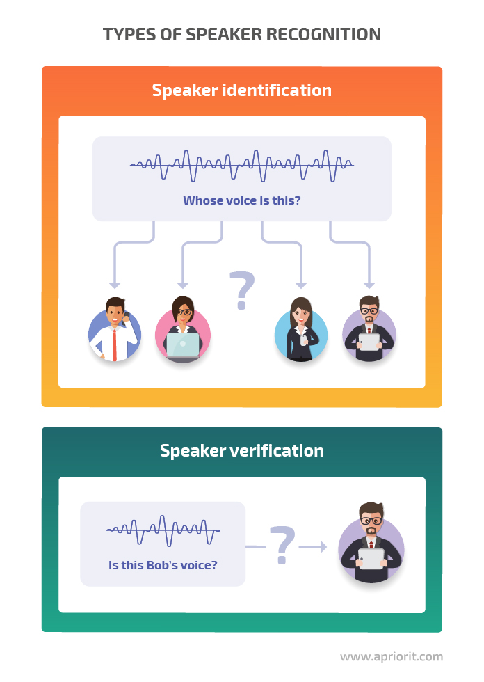
You can build a speaker recognition system using static signal processing, machine learning algorithms, neural networks, and other technologies. In this article, we focus on the specifics of accomplishing speaker recognition tasks using machine learning algorithms.
Both speaker verification and speaker identification systems consist of three main stages:
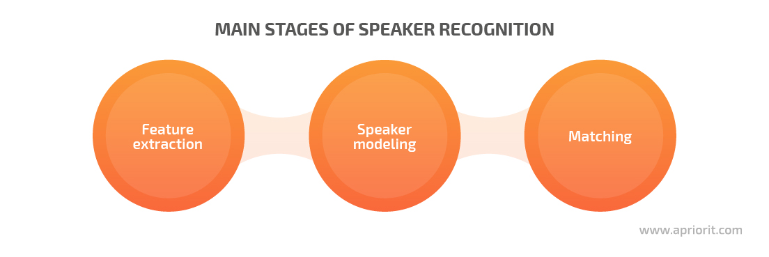
- Feature extraction is when the system extracts essential voice features from raw audio
- Speaker modeling is when the system creates a probabilistic model for each speaker
- Matching is when the system compares the input voice with every previously created model and chooses the model that best matches the input voice
Implementing each of these stages requires different tools and techniques. We look closely at some of them in the next section.
Speech is the key element in speaker recognition. And to work with speech, you’ll need to reduce noise, distinguish parts of speech from silence, and extract particular speech features. But first, you’ll need to properly prepare your speech recordings for further processing.
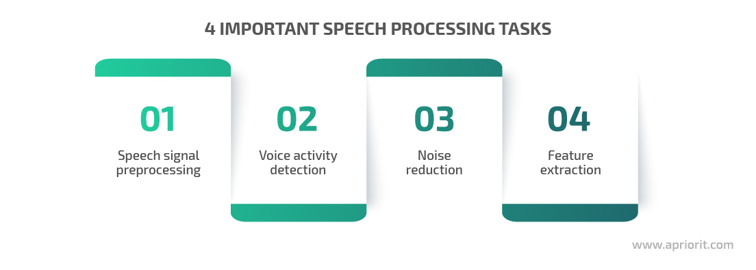
Speech signal preprocessing
Converting speech audio to the data format used by the ML system is the initial step of the speaker recognition process.
Start by recording speech with a microphone and turning the audio signal into digital data with an analog-to-digital converter. Further signal processing commonly includes processes like voice activity detection (VAD), noise reduction, and feature extraction. We’ll look at each of these processes later.
First, let’s overview some of the key speech signal preprocessing techniques: feature scaling and stereo-to-mono conversion.
Since the range of signal values varies widely, some machine learning algorithms can’t properly recognize audio without normalization. Feature scaling is a method used to normalize the range of independent variables or features of data. Scaling data eliminates sparsity by bringing all your values onto the same scale, following the same concept as normalization and standardization.
For example, you can standardize your audio data using the sklearn.preprocessing package. It contains utility functions and transformer classes that allow you to improve the representation of raw feature vectors.
Here’s how this works in practice:
Python
from sklearn import preprocessing
def extract_features(audio,rate):
   mfcc_feature = mfcc.mfcc(audio,rate, winlen=0.020,preemph=0.95,numcep=20,nfft=1024,ceplifter=15,highfreq=6000,nfilt=55,appendEnergy=False)
   mfcc_feature = preprocessing.scale(mfcc_feature)
   delta = calculate_delta(mfcc_feature)
   combined = np.hstack((mfcc_feature,delta))
   return combined
The number of channels in an audio file can also influence the performance of your speaker recognition system. Audio files can be recorded in mono or stereo format: mono audio has only one channel, while stereo audio has two or more channels. Converting stereo recordings to mono helps to improve the accuracy and performance of a speaker recognition system.
Python provides a pydub module that enables you to play, split, merge, and edit WAV audio files. This is how you can use it to convert a stereo WAV file to a mono file:
Python
from pydub import AudioSegment
mysound = AudioSegment.from_wav("stereo_infile.wav")
# set mono channel
mysound = mysound.set_channels(1)
# save the result
mysound.export("mono_outfile.wav", format="wav")
Now that we’ve overviewed key preparation measures, we can dive deeper into the specifics of speech signal processing techniques.
Voice activity detection
To let the feature extraction algorithm for speaker recognition focus only on speech, we can remove silence and non-speech parts of the audio. This is where VAD comes in handy. This technique can distinguish human speech from other signals and is often used in speech-controlled applications and devices like voice assistants and smartphones.
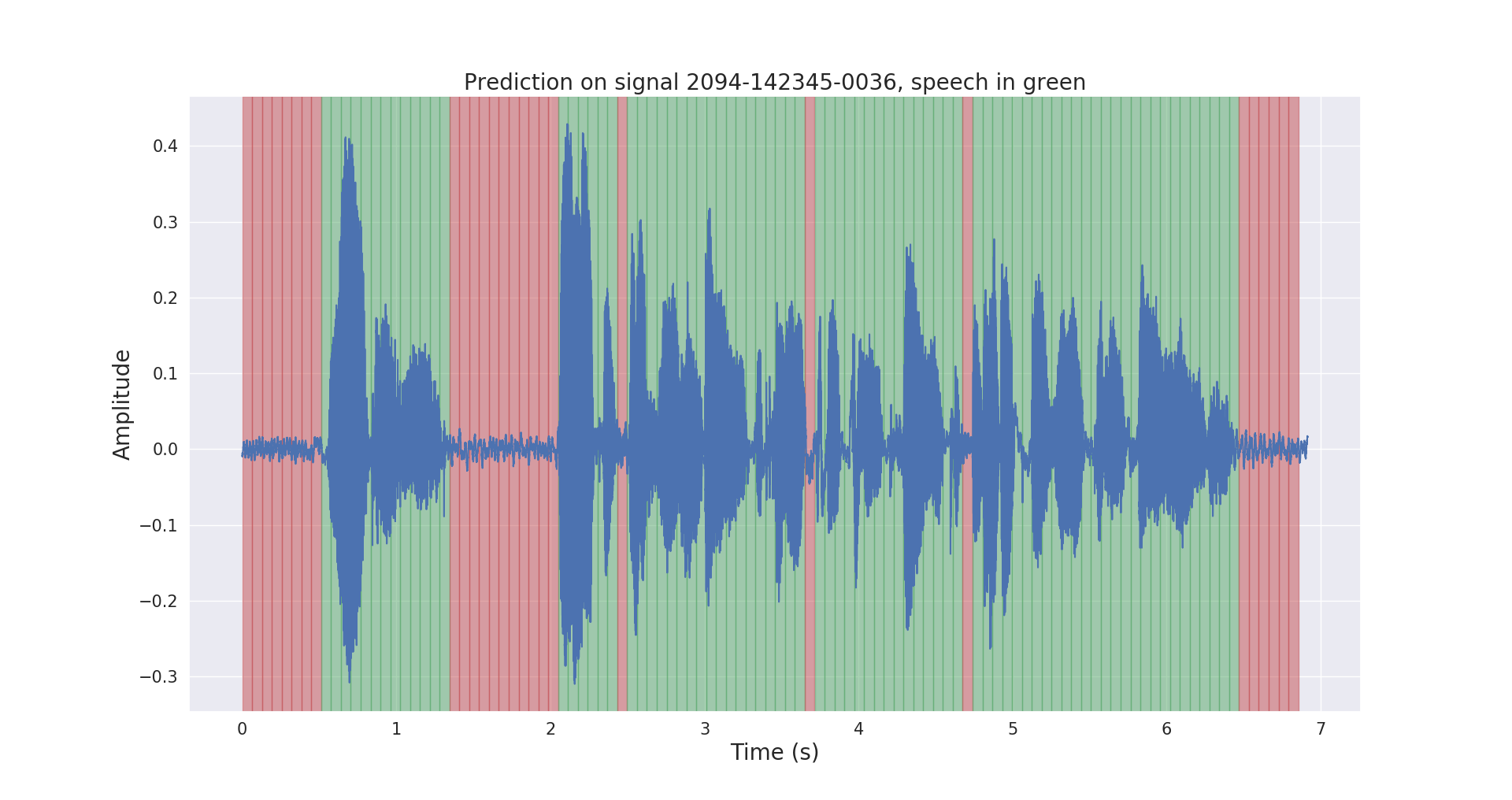
Figure 1. Speech signal prediction scheme. Image credit: Python Awesome
The main goal of a voice activity detection algorithm is to determine which segments of a signal are speech and which are not. A VAD algorithm can improve the performance of a speaker verification system by making sure that the speaker’s identity is calculated using only the frames that contain speech. Therefore, you should evaluate the necessity of using a VAD algorithm to overcome problems in designing a robust speaker verification system.
As for the practical aspects of VAD implementation, you can turn your attention to PyTorch, a high-performance open-source library with a rich variety of deep learning (DL) algorithms.
Here’s how you can use PyTorch to detect voice activity in a recording:
Python
import torch


# loading vad model and tools to work with audio
model, utils = torch.hub.load(repo_or_dir='snakers4/silero-vad', model='silero_vad', force_reload=False)

(_, get_speech_ts_adaptive, save_audio, read_audio, _, _, collect_chunks) = utils

audio = read_audio('raw_voice.wav')


# get time chunks with voice
speech_timestamps = get_speech_ts_adaptive(wav, model)


# gather the chunks and save them to a file
save_audio('only_speech.wav',
       	collect_chunks(speech_timestamps, audio))
Noise reduction
Noise is inevitably present in almost all acoustic environments. Even when recorded with a microphone, a speech signal will contain lots of noise, such as white noise or background sounds.
Excessive noise can distort or mask the characteristics of speech signals, degrading the overall quality of the speech recording. The more noise an audio signal contains, the poorer the performance of a human-to-machine communication system.
Noise detection and reduction are often formulated as a digital filtering problem, where you get clean speech by passing noisy speech through a linear filter. In this case, the key challenge is to design a filter that can significantly suppress noise without causing any noticeable speech distortion.
Developing a versatile noise detection and reduction algorithm that works in diverse environments is a challenging task, as noise characteristics are inconsistent.
You can use these two tools to successfully handle noise detection and reduction tasks:
- Noisereduce is a Python noise reduction algorithm that you can use to reduce the level of noise in speech and time-domain signals. It includes two algorithms for stationary and non-stationary noise reduction.
- SciPy is an open-source collection of mathematical algorithms that you can use to manipulate and visualize data using high-level Python commands.
Here’s an example of working with SciPy:
Python
import noisereduce as nr
from scipy.io import wavfile

# load data
rate, data = wavfile.read("voice_with_noise.wav")

# perform noise reduction
reduced_noise = nr.reduce_noise(y=data, sr=rate)
Feature extraction
Feature extraction is the process of identifying unique characteristics in a speech signal, transforming raw acoustic signals into a compact representation. There are various techniques to extract features from speech samples: Linear Predictive Coding, Mel Frequency Cepstral Coefficient (MFCC), Power Normalized Cepstral Coefficients, and Gammatone Frequency Cepstral Coefficients, to name a few.
In this section, we’ll focus on two popular feature extraction techniques:
- Mel-frequency cepstrum (MFCC)
- Delta MFCC
MFCC is a feature extractor commonly used for speech recognition. It works somewhat similarly to the human ear, representing sound in both linear and non-linear cepstrals.
If we take the first derivative of an MFCC feature, we can extract a Delta MFCC feature from it. In contrast to general MFCC features, Delta MFCC features can be used to represent temporal information. In particular, you can use these features to represent changes between frames.
You can find these three tools helpful when working on feature extraction in a speaker recognition system:
- NumPy is an open-source Python module providing you with a high-performance multidimensional array object and a wide selection of functions for working with arrays.
- Scikit-learn is a free ML library for Python that features different classification, regression, and clustering algorithms. You can use Scikit-learn along with the NumPy and SciPy libraries.
- Python_speech_features is another Python library that you can use for working with MFCCs.
Here’s an example of using delta MFCC and combining it with a regular MFCC:
Python
import numpy as np
from sklearn import preprocessing
from python_speech_features import mfcc, delta

def extract_features(audio,rate):
	"""extract 20 dim mfcc features from audio file, perform CMS and combine
	delta to make 40 dim feature vector"""

	mfcc_feature = mfcc.mfcc(audio, rate, winlen=0.020,preemph=0.95,numcep=20,nfft=1024,ceplifter=15,highfreq=6000,nfilt=55,appendEnergy=False)

	# feature scaling
	mfcc_feature = preprocessing.scale(mfcc_feature)
	delta_feature = delta(mfcc_feature, 2) # calculating delta
	# stacking delta features with common features
	combined_features = np.hstack((mfcc_feature, delta_feature))
	return combined_features
Now that you know what speaker recognition techniques and tools you can use, it’s time to see the ML and DL models and algorithms that can help you build an efficient speaker recognition system. You can also use these techniques to figure out how to make an IVR system for real time voice responce.
ML and DL models for speaker recognition
While you can always try building a custom machine learning model from scratch, using an already trained and tested algorithm or model can save both time and money for your speaker recognition project. Below, we take a look at five ML and DL models commonly applied for speech processing and speaker recognition tasks.
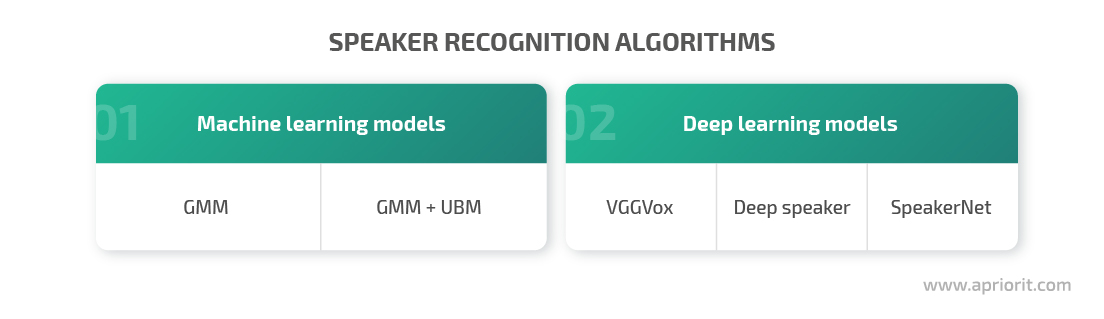
We’ll start with one of the most popular models for processing audio data — the Gaussian Mixture Model.
Gaussian Mixture Model
The Gaussian Mixture Model (GMM) is an unsupervised machine learning model commonly used for solving data clustering and data mining tasks. This model relies on Gaussian distributions, assuming there is a certain number of them, each representing a separate cluster. GMMs tend to group data points from a single distribution together.
Combining a GMM with the MFCC feature extraction technique provides great accuracy when completing speaker recognition tasks. The GMM is trained using the expectation maximization algorithm, which creates gaussian mixtures by updating gaussian means based on the maximum likelihood estimate.
To work with GMM algorithms, you can use the sklearn.mixture package, which helps you learn from and sample different GMMs.
Here’s how you extract features (using the previously described method) and train the GMM using sklearn.mixture:
Python
sample_rate, data = read('denoised_vad_voice.wav')

# extract 40 dimensional MFCC & delta MFCC features
features = extract_features(audio, sr)

gmm = GMM(n_components=16,max_iter=200,covariance_type='diag',n_init=1, init_params='random')
gmm.fit(features)  # gmm training
Combining the Gaussian Mixture Model and Universal Background Model
A GMM is usually trained on speech samples from a particular speaker, distinguishing speech features unique to that person.
When trained on a large set of speech samples, a GMM can learn general speech characteristics and turn into a Universal Background Model (UBM). UBMs are commonly used in biometric verification solutions to represent person-independent speech features.
Combined in a single system, GMM and UBM models can better handle alternative speech they may encounter during speaker recognition, like whispers, slow speech, or fast speech. This applies to both the type and the quality of speech as well as the composition of speakers.
Note that in typical speaker verification tasks, a speaker model can’t be identified directly with the help of the expectation maximization algorithm, as the variety of training data is limited. For this reason, speaker models in speaker verification systems are often trained using the maximum a posteriori (MAP) adaptation, which can estimate a speaker model from UBM.
As for tools, you can use Kaldi — a popular speech recognition toolset for clustering and feature extraction. To integrate its functionality with Python-based workflows, you can go with the Bob.kaldi package that provides pythonic bindings for Kaldi.
Here’s an example of working with Bob.kaldi:
Python
ubm = bob.kaldi.ubm_train(features, r'ubm_vad.h5', num_threads=4, num_gauss=2048, num_iters=100)


# training every gmm using ubm
user_model = bob.kaldi.ubm_enroll(features, ubm)


# scoring using ubm and a specified gmm
bob.kaldi.gmm_score(features, user_model, ubm)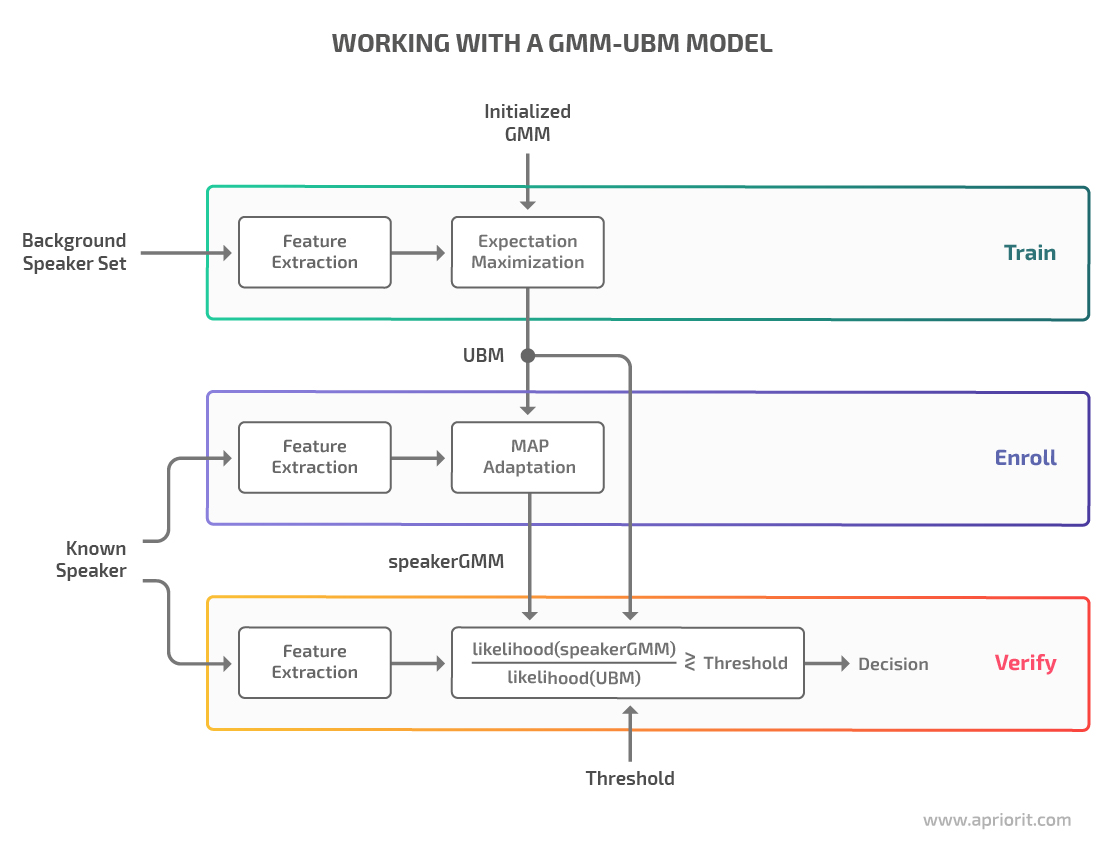
To achieve even higher accuracy, you can try accomplishing speaker recognition tasks with deep learning algorithms. Let’s look at some of the commonly applied DL models in the next section.
Deep learning models for speaker recognition
When trying to solve speaker recognition problems with deep learning algorithms, you’ll probably need to use a convolutional neural network (CNN). While this type of neural network is widely applied for solving image-related problems, some models were designed specifically for speech processing:
VGGVox is a DL system that can be used for both speaker verification and speaker identification. The network architecture allows you to extract frame-level features from the spectrograms and aggregate them to obtain an audio voice print. To verify a speaker, the system compares voice prints using cosine distance — for similar voice prints, this distance will always be rather small.
To train this model, you need to preprocess your audio data by converting regular audio to the mono format and generating spectrograms out of it. Then you can feed normalized spectrograms to the CNN model in the form of images.
Deep speaker is a Residual CNN–based model for speech processing and recognition. After passing speech features through the network, we get speaker embeddings that are additionally normalized in order to have unit norm.
Just like VGGVox, the system checks the similarity of speakers using the cosine distance method. But unlike VGGVox, Deep speaker computes loss using the triplet loss method. The main idea of this method is to maximize the cosine similarities of two different embeddings of the same speaker while minimizing embeddings of another speaker.
Audio preprocessing for this system includes converting your audio files to 64-dimensional filter bank coefficients and normalizing the results so they have zero mean and unit variance.
SpeakerNet is a neural network that can be used for both speaker verification and speaker identification and can easily be integrated with other deep automatic speech recognition models.
The preprocessing stage for this model also includes generating spectrograms from raw audio and feeding them to the neural network as images.
When working with these models, you can rely on the glob module that helps you find all path names matching a particular pattern. You can also use the malaya_speech library that provides a rich selection of speech processing features.
Here’s what working with these DL models can look like in practice:
Python
# load model
def deep_model(model: str = 'speakernet', quantized: bool = False, **kwargs):
	"""
	Load Speaker2Vec model.

	Parameters
	----------
	model : str, optional (default='speakernet')
    	Model architecture supported. Allowed values:

    	* ``'vggvox-v1'`` - VGGVox V1, embedding size 1024
    	* ``'vggvox-v2'`` - VGGVox V2, embedding size 512
    	* ``'deep-speaker'`` - Deep Speaker, embedding size 512
    	* ``'speakernet'`` - SpeakerNet, embedding size 7205

	quantized : bool, optional (default=False)
    	if True, will load 8-bit quantized model.
    	The quantized model isn’t necessarily faster, it totally depends on the machine.

	Returns
	-------
	result : malaya_speech.supervised.classification.load function
	"""

model = malaya_speech.speaker_vector.deep_model('speakernet')

from glob import glob

speakers = ['voice_0.wav', 'vocie_1.wav', 'voice_2.wav']

# pipeline
def load_wav(file):
	return malaya_speech.load(file)[0]

p = Pipeline()
frame = p.foreach_map(load_wav).map(model)
r = p.emit(speakers)

# calculate similarity
from scipy.spatial.distance import cdist

1 - cdist(r['speaker-vector'], r['speaker-vector'], metric = 'cosine')
However, choosing the right ML or DL model is not enough for building a well-performing speaker recognition system. In the next section, we discuss how setting the right parameters can greatly improve the performance of your machine learning models.
Improving model performance with parameter tuning
There are factors affecting speaker recognition accuracy and the performance of your model. One of these factors is hyperparameters — parameters that a machine learning model can’t learn directly within estimators. These parameters are usually specified manually when developing the ML model.
Setting the appropriate values for hyperparameters can significantly improve your model’s performance. Let’s take a look at ways you can choose the right parameters and cross-validate your model’s performance based on the example of the Scikit-learn library.
Choosing parameters with grid search
Note: To follow through with our examples, you need to install the Scikit-learn library.
There’s no way to know the best values for hyperparameters in advance. Therefore, you need to try all possible combinations to find the optimal values.
One way to train an ML model with different parameters and determine parameters with the best score is by using grid search.
Grid search is implemented using GridSearchCV, available in Scikit-learn’s model_selection package. In this process, the model only uses the parameters specified in the param_grid parameter. GridSearchCV can help you loop through the predefined hyperparameters and fit your estimator to your training set. Once you tune all the parameters, you’ll get a list of the best-fitting hyperparameters.
Along with performing grid search, GridSearchCV can perform cross-validation — the process of choosing the best-performing parameters by dividing the training and testing data in different ways.
For example, we can choose an 80/20 data splitting coefficient, meaning we’ll use 80% of data from a chosen dataset for training the model and the remaining 20% for testing the model. Once we decide on the coefficient, the cross-validation technique applies a specified number of combinations to this data to find out the best split.
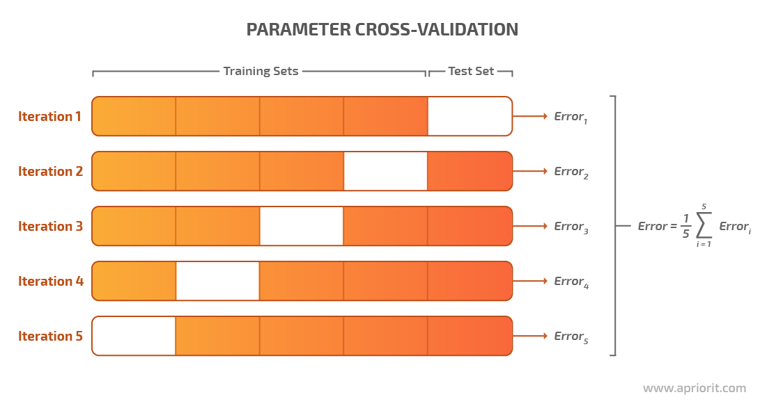
This is where the pipeline comes into play.
Cross-validating a model with pipelines
A pipeline is used to assemble several steps that can be cross-validated while setting different parameters for a model.
There are must-have methods for pipelines:
-
- The fit method allows you to learn from data
- The transform or predict method processes the data and generates a prediction
Scikit-learn’s pipeline class is useful for encapsulating multiple transformers alongside an estimator into one object so you need to call critical methods like fit and predict only once.
We can get the pipeline class from the sklearn.pipeline module.
You can chain transformers and estimators into a sequence that functions as a single cohesive unit using Scikit-learn’s pipeline constructor. For example, if your model involves feature selection, standardization, and regression, you can encapsulate three corresponding classes using the pipeline module.
And if you are using custom functions to transform data at the preprocessing and feature extraction stages, you might need to write custom transfer and classifier classes to incorporate these actions into your pipeline.
Here’s an example of a custom transformer class:
Python
import numpy as np
import warnings
from python_speech_features import mfcc, delta
from sklearn import preprocessing
from sklearn.utils.validation import check_is_fitted

warnings.filterwarnings('ignore')
from sklearn.base import BaseEstimator, TransformerMixin
And this is what a CustomTransformer(TransformerMixin, BaseEstimator) class would look like:
Python
def __init__(self, winlen=0.020,preemph=0.95,numcep=20,nfft=1024,ceplifter=15,highfreq=6000,nfilt=55,appendEnergy=False):
    	self.winlen = winlen
    	self.preemph = preemph
    	self.numcep = numcep
    	self.nfft = nfft
    	self.ceplifter = ceplifter
    	self.highfreq = highfreq
    	self.nfilt = nfilt
    	self.appendEnergy = appendEnergy

	def transform(self, x):
    	""" A reference implementation of a transform function.
            	Parameters
            	----------
            	x : {array-like, sparse-matrix}, shape (n_samples, n_features)
                	The input samples.
            	Returns
            	-------
            	X_transformed : array, shape (n_samples, n_features)
                	The array containing the element-wise square roots of the values
                	in ``X``.
            	"""
    	# Check is fit has been called
    	check_is_fitted(self, 'n_features_')

    	# Check that the input is of the same shape as the one passed
    	# during fit.
    	if x.shape[1] != self.n_features_:
        	raise ValueError('Shape of input is different from what was seen'
                         	'in `fit`')
    	return self.signal_to_mfcc(x)

	def fit(self, x, y=None):
    	"""A reference implementation of a fitting function for a transformer.
            	Parameters
            	----------
            	x : {array-like, sparse matrix}, shape (n_samples, n_features)
                	The training input samples.
            	y : None
                	There is no need of a target in a transformer, yet the pipeline API
                	requires this parameter.
            	Returns
            	-------
            	self : object
                	Returns self.
            	"""
    	self.n_features_ = x.shape[1]
    	return self
If you need a custom classifier class, this is what it might look like:
Python
import numpy as np
import warnings
from python_speech_features import mfcc, delta
from sklearn import preprocessing
from sklearn.utils.validation import check_is_fitted

warnings.filterwarnings('ignore')
from sklearn.base import BaseEstimator, TransformerMixin
You might also need to create additional methods to load data and extract features and sample rates.
Here’s how you can create a load data method:
Python
def load_data(folder):
	x, y = [], []

	for voice_sample in list(glob.glob(rf'./{folder}/id*/id*')):
    	voice_sample_file_name = os.path.basename(voice_sample)
    	voice_class, _ = voice_sample_file_name.split("_")

    	features = read_wav(voice_sample)

    	x.append(features)
    	y.append(voice_class)

	return np.array(x, dtype=tuple), np.array(y)
And here’s what the code of a method to extract features and sample rate can look like:
Python
def read_wav(fname):
	fs, signal = wavfile.read(fname)
	if len(signal.shape) != 1:
    	signal = signal[:,0]
	return fs, signal
The parameters for the param_grid module should be specified using documentation for the defined method. It’s important to mention the list of different values or the range of values.
If you’re using binary outcomes (true or false), you need to define only two values. When working with categorical values, you need to create a list of all possible string values.
Here’s an example of how to determine the best-fitting parameters using grid search and a pipeline:
Python
x, y = load_data('test')


# creating pipeline of transformer and classifier
pipe = Pipeline([('scaler', CustomTransformer()), ('svc', CustomClassifier())])


# creating the parameters grid
param_grid = {
    'scaler__appendEnergy': [True, False],
    'scaler__winlen': [0.020, 0.025, 0.015, 0.01],
    'scaler__preemph': [0.95, 0.97, 1, 0.90, 0.5, 0.1],
    'scaler__numcep': [20, 13, 16],
    'scaler__nfft': [1024, 1200, 512],
    'scaler__ceplifter': [15, 22, 0],
    'scaler__highfreq': [6000],
    'scaler__nfilt':[55, 0, 22],
    'svc__n_components': [2 * i for i in range(0, 12, 1)],
    'svc__max_iter': list(range(50, 400, 50)),
    'svc__covariance_type': ['full', 'tied', 'diag', 'spherical'],
    'svc__n_init': list(range(1, 4, 1)),
    'svc__init_params': ['kmeans', 'random']
}
search = GridSearchCV(pipe, param_grid, n_jobs=-1)
# searching for appropriate parameters
search.fit(x, y)
To illustrate how different parameters can affect the performance of an ML model, we tested the previously discussed models on different datasets. Go to the next section to see the results of these tests.
Evaluating the impact of parameter tuning
We tested the performance of two machine learning models: a combination of GMM and MFCC and the GMM-UBM model. For better test result accuracy, we compared the performance of these models on two datasets:
1. LibriSpeech — This dataset is a collection of around 1,000 hours of audiobook recordings. The training data is split into three sets: two containing “clean” speech (100 hours and 360 hours) and one containing 500 hours of “other” speech, which is considered more challenging for an ML model to process. The test data is also split into two categories: clean and other.
Here’s the structure of the LibriSpeech dataset:
ShellScript
.- train-clean-100/
            	|
            	.- 19/
                	|
                	.- 198/
                	| |
                	| .- 19-198.trans.txt
                	| |
                	| .- 19-198-0001.flac
                	| |
                	| .- 14-208-0002.flac
                	| |
                	| ...
                	|
                	.- 227/
                     	| ...
2. VoxCeleb1 — This is one of two audio-visual VoxCeleb datasets formed from YouTube interviews with celebrities. In contrast to LibriSpeech, this dataset doesn’t have many clean speech samples, as most interviews were recorded in noisy environments.
The dataset includes recordings of 1251 celebrities, with a separate file for each person. Each file has subfolders with WAV audio files, and each subfolder depicts the YouTube video that was used to create the speech samples.
Here’s the structure of this dataset:
ShellScript
.- vox1-dev-wav/
|        	|
|        	.- wav/
|            	|
|            	.- id10001/
|            	| 	|
|            	| 	.- 1zcIwhmdeo4/
|            	| 	|    	|
|            	| 	...  	.- 00001.wav
|            	|
|            	.- id10002/
|                  	|
|                  	...
|
First, we tested a simple GMM-MFCC model trained on the LibriSpeech dataset. The results are the following:
Table 1 – Testing a GMM-MFCC model on the LibriSpeech dataset
| Number of users | Level of accuracy |
| 100 users | 98.0% accuracy |
| 1000 users | 95.8% accuracy |
As this dataset contains clean speech samples, the results for LibriSpeech are always good, whether we use a GMM-MFCC, GMM-UBM, or any other machine learning model. For this reason, all other tests will be focused on the VoxCeleb dataset, which is a lot more challenging for a machine learning model to process.
Let’s start with the results of testing a GMM-MFCC model using the VoxCeleb dataset:
Table 2 – Testing a GMM-MFCC model on the VoxCeleb dataset
| Number of users | Level of accuracy |
| 100 users | 84.8% accuracy |
| 1000 users | 72.1% accuracy |
As you can see, the accuracy of our model decreased significantly, especially when applied to a larger number of users.
Now let’s take a look at the results of testing a GMM-UBM model trained on the VoxCeleb dataset:
Table 3 – Testing a GMM-UBM model on the VoxCeleb dataset
| Number of users | Level of accuracy |
| 100 users | 92% accuracy |
| 1000 users | 84% accuracy |
This model proved to be more accurate than the GMM-MFCC model.
We can also see how changing the parameters of a model affects its performance. For this example, we tested the MFCC model and its delta and delta + double delta versions on 100 users:
Table 4 – Testing the influence of parameter changes
| Parameters | MFCC | MFCC + delta | MFCC + delta + double delta |
| numcep=13 | 81.6% accuracy | 77.6% accuracy | 80.3% accuracy |
| numcep=20 | 87.6% accuracy | 87.0% / 89.0% accuracy | 83.0% accuracy |
The numcep value represents the number of cepstrums to return. As you can see, the higher the numcep, the more accurate the results our models show.
And as for the deep learning models mentioned in this article, they showed the following results when trained on the VoxCeleb dataset and tested on 100 users:
Table 5 – Testing DL models on the VoxCeleb dataset
| Model | Level of accuracy |
| SpeakerNet | 97% accuracy |
| VGGVox | 96% accuracy |
| Deep speaker | 75% accuracy |
As you can see, the performance of different ML and DL methods depends greatly on both the parameters specified for your model and the dataset you use to train it. So before making a final choice on the ML or DL model for your speaker recognition project, it would be best to test several models on different datasets to find the best-performing combination.
Conclusion
Speech recognition is the core element of complex speaker recognition solutions and is commonly implemented with the help of ML algorithms and deep neural networks. Depending on the complexity of the task at hand, you can combine different speaker recognition technologies, algorithms, and tools to improve the performance of your speech processing system.
When in doubt, consult a professional! Apriorit’s AI development team will gladly assist you with choosing the right set of parameters, tools, datasets, and models for your AI project. Reach out to us using the form below, or leave a message in the chat window!
Speech Recognition using Neural Networks
Speech Recognition using Neural Networks
Mr. Hardik Dudhrejia
Department of Computer Engineering
G H Patel College of Engineering & Technology Vadodara, India
Mr. Sanket Shah
Department of Computer Engineering
G H Patel College of Engineering & Technology Anand, India
AbstractSpeech is the most common way for humans to interact. Since it is the most effective method for communication, it can be also extended further to interact with the system. As a result, it has become extremely popular in no time. The speech recognition allows system to interact and process the data provided verbally by the user. Ever since the user can interact with the help of voice the user is not confined to the alphanumeric keys. Speech recognition can be defined as a process of recognizing the human voice to generate commands or word strings. It is also popularly known as ASR (Automatic speech recognition), computer speech recognition or speech to text (STT). Speech recognition activity can be performed after having a knowledge of diverse fields like linguistic and computer science. It is not an isolated activity. Various techniques available for speech recognition are HMM (Hidden Markov model)[1], DTW(Dynamic time warping)- based speech recognition[2], Neural Networks[3], Deep feedforward and recurrent neural networks[4] and End-to-end automatic speech recognition[5]. This paper mainly focusses on Different Neural networks used for Automatic speech recognition. This research paper primarily focusses on different types of neural networks used for speech recognition. In addition to this paper also consist of work done on speech recognition using this neural networks.
Keywords Speech recognition; Recurrent Neural network; Hidden Markov Model; Long Short term memory network
-
INTRODUCTION
Throughout their life-span humans communicate mostly through voice since they learn all the relevant skills in their early age and continue to rely on speech communication. So, it is more efficient to communicate with speech rather than by using keyboard and mouse. Voice Recognition or Speech Recognition provides the methods using which computers can be upgraded to accept speech or human voice assist input instead of giving input by keyboard. It is extremely advantageous for the disabled people.
Speech is affected greatly by the factors such as pronunciations, accents, roughness, pitch, volume, background noise, echoes and gender. Preliminary method of speech processing is the process of studying the speech signals and the methods of processing these signals.
The conventional method of speech recognition insist in representing each word by its feature vector and pattern matching with the statistically available vectors using neural networks. On the contrary to the antediluvian method HMM, neural networks does not require prior knowledge of speech process and do not need statistics of speech data. [3]
Types of speech recognition: Based on the type of words speech recognizing systems can recognize, the speech recognition system is divided into the following categories:
-
Isolated Word:
Isolated word requires each utterance to have quiet on both sides of sample window. At a time only single words and single utterances are accepted and it is having Listen and Non-Listen state.
-
Continuous Word:
Continuous speech recognisers provide the users a facility to speak in a continuous fashion and almost naturally and at the same time the computer determines the content of the speech. Recognisers rendering the facility of continuous speech capabilities are pretty much difficult to create because they require some special and peculiar methods in order to determine the boundaries of the utterances.
-
Connected Word:
Connected words are very much alike the isolated words but they allow separate utterances to be executed with minimal pauses in between them.
-
Spontaneous speech:
At an elementary level, spontaneous speech can be considered as a speech that is coming out naturally and not a rehearsed one. An Automatic Speech Recogniser must be able to handle a wide range of speech features like the words being run together.
Classification of speech sounds:
In this modern time, the process of classification of speech sounds is commonly done on the basis of 2 process based on how the classification process is looked upon:
Based on the process of obstruction and non-obstruction sounds
The process of classifying the sounds with respect to the process of obstruction and non-obstruction relies upon the conception of bodily air. While generating human sounds, the air coming out of the body has two functions; it is obstructed in the mouth or throat somewhere or it doesnt get obstructed, but the air comes out very easily. Correspondingly, the sounds that are produces as a result of obstructions and non-obstructions are not same excluding some of their qualities that are trivial.
For e.g.- all the vowels (a,e,i,o,u) are non obstruction speech sounds and all the consonants (b,c,d,f,g,h,j,k,l,m,n,p,q,r,s,t,v,w,x,y,z) are obstruction speech sounds.
Based on the process of voice and voiceless sounds
Voiced sound is produced when the vocal chords vibrate when the sound is produced. Whereas in the voiceless sound no vocal cord vibration is produced. To test this, place your finger on your throat as you say the words. A vibration will be felt when the voiced sounds are uttered and no vibration will be felt while uttering a voiceless sound. Many a times it is difficult to feel the difference between them. So in order to distinguish between them another test can be performed by putting a paper in front of our mouth and the paper should move only by saying the voiceless sounds. All the vowels are voiced whereas some of the consonants are voiced as well as voiceless.
Voiced consonants are :- b,d,g,v,z,th,sz,j,l,m,n,ng,r,w,y Voiceless consonants are :- p,t,k,f,s,th,sh,ch,h
-
-
SPEECH RECOGNITION PROCESS
Speech Recognition is truly a ponderous and tiresome process. It consists of 5 steps:-
-
Speech
-
Speech Pre-Processing
-
Feature Extraction
-
Speech Classification
-
Recognition
numerous tools and softwares available which record the speech delivered by the humans. The phonic environment and the equipment device used have a significant impact on the speech generated. There is a possibility of having background or room reverberation blended with the speech but this is completely undesirable.
Speech Pre-Processing
The solution of the problem described above is the Speech Pre-Processing. It plays an influential role in cancelling out the trivial sources of variation. The speech pre-processing typically includes reverberation cancelling, echo cancellation, windowing, noise filtering and smoothing all of which conclusively improves the accuracy of speech recognition.
Feature Extraction
Each and every person has different speech and different intonation. This is due to the different characteristics ingrained in their utterance. There should be a probability of identifying speech from the theoretical waveform, at least theoretically. As a result of an enormous variation in speech there is an imminent need to reduce the variations by performing some feature extraction. The ensuing section depicts some of the feature extraction technologies which are extremely used nowadays.
LPC (Linear Predictive Coding):- It s an extremely useful speech analysis technique for encoding quality speech at low bit rate and is one of the most powerful method. The key idea behind this method is that a specific speech sample at current time can be approximated as a linear combination of past speech samples. In this method the digital signal is compressed for competent storage and transmission. The principle behind the use of LPC is to reduce the sum of squared distance between the original speech and estimated speech over a finite duration. It can be further used to provide unique set of predictor coefficients. Gain (G) is also a crucial parameter.
MFCC (Mel Frequency Cepstarl Coefficients):- This is the standard method feature extraction. It is preliminary based on the frequency domain which is based Mel scale based on human ear scale. They are more accurate than time domain features ever since they fall into the category of frequency domain features. The most conspicuous impediment is its sensitivity to noise as it is highly dependent on the spectral form. Techniques utilizing the periodicity of speech signals could be used to overcome this drawback although speech also encompasses aperiodic content.
Speech
Figure-1 Speech recognition process
Speech Classification
These systems are used to extract the hidden information from the input processing signals and comprises of convoluted mathematical functions. This section describes some commonly used speech classification techniques in brief.
Speech is defined as the ability to express ones thoughts and feelings by articulate sounds. Initially the speech of a person is received in the form of a waveform. Also there are
HMM (Hidden Markov Model):- This is the most strongly
used method in order to recognize pattern in the speech. It is safer and possesses a secure mathematical foundation as
compared to the template based and knowledge based approach. In this method, the system being modelled is assumed to be a Markov process having hidden states. The speech is distributed into smaller resounding entities each of which represent a state. In simpler Markov Model, the states are clearly visible to the user and thus the state transition probabilities are only the parameters. On the other hand, in hidden Markov Model, the state is not directly visible, but the output, which is dependent on the state, is evident. HMM are specifically known for their application in reinforcement learning and pattern recognition such as speech, handwriting and bioinformatics.
DTW (Dynamic Time Warping):-In time series analysis, DTW is a kind of algorithm which measures the similarity or affinity between two temporal sequences that vary in speed or time. It correlates the speech words with reference words. This method changes the time dimension of the undiscovered words unless and until they are matched with the reference word. A well-known application of DTW is the automatic speech recognition, in order to cope up with different speaking speeds. Various other applications are online signature recognition and speaker recognition.
VQ (Vector Quantization):- This method is preliminary based on block coding principle. This technique allows the modelling of probability density functions by the circulation of prototype vectors. It was formerly used for data compression. It performs the mapping of the vector from a vast vector space to a finite number of regions in that space. Every region is known as cluster and can be depicted by its centre called code word. Vector Quantization is used in lossy data compression, lossy data correction, and clustering and pattern recognition.
Recognition
After the above four phases speech recording, speech pre- processing, feature extraction and speech classification the final step that is remaining is the speech recognition. Once all the above mentioned steps are completed successfully then the recognition of speech can be done by three approaches.
-
Acoustic phonetic approach[6]
-
Pattern recognition approach[7]
-
Artificial intelligence approach
This paper is mainly concern with Artificial intelligence approach for speech recognition. This is a combination of acoustic phonetic and pattern recognition approach. In this approach system created by neural networks are used to classify and recognize the sound.. Neural networks are very powerful for recognition of speech. There are various networks for this process. RNN, LSTM, Deep Neural network and hybrid HMM-LSTM are used for speech recognition.
-
-
-
NEURAL NETWORKS
Traditionally neural networks referred to as neurons or circuit. At present the term neural networks refers to as Artificial Neural Network, consisting of artificial neurons or
nodes. It is a network of elementary elements known as artificial neurons, which receives an input, changes the state according to that input and generates an output. An interconnected group of natural or artificial neurons uses a mathematical model for information processing based on connectionist approach to communication. Neutral Networks can be treated as simple mathematical models defining a function f: X Y or a distribution over X or both X and Y [8], but many a times models are intimately connected with a particular learning rule. The term artificial neural network refers to inter-connections in among the neurons in the different layers of each system. Mathematically a neurons network function f(x) is defined as a composition of other functions gi(x), which can further be defined as a composition of other functions. A most commonly used type of composition is the nonlinear weighted sum, where f(x) = K (i ,wigi(x)), where K is a predefined function. Referring the collection of functions gi as a vector g simply would be more advantageous. The first view being the functional view; the given x is then changed to a 3-D vector h, which is then finally transformed into f. This view is frequently encountered in the optimization context. Probabilistic view is the second view and the arbitrary variable G = g (H), depends on H = h(X), which in turn depends upon the X(random variable). In the perspective of graphical models this view most commonly comes across. Networks described such as the above one are often called feed forward as its graph is a DAG (Directed Acyclic Graph). Networks which have cycles in it is called recurrent neural networks.
Neural Network Models:
Language modelling and acoustic modelling are both vital aspects of modern statistically-based speech recognition systems. The ensuring section illustrates various methods for Speech Recognition.
Deep Neural Network (Hidden Markov Models HMM is a generative model in which observable acoustic features are assumed to be generated from a hidden Markov process that transitions between states S = {s1, s2 ., sk}.
HMM was the most widely used technique for Large Vocabulary Speech Recognition (LSVR) for at least two decades. The decisive parameters in the HMM are the initial state probability distribution f = {p(q0=si)}, where qt is the state at time t; the transition probabilities aij= p(qt=sj |qt- 1=si) ; and a model to estimate the observation probabilities p(xt |si). The conventional HMM used in the process of Automatic Speech Recognition had their observation probability modelled by using Gaussian Mixture Model (GMM). Even the GMM had a vast number of advantages, the issue was that, they were statistically inept for modelling data that lie on or near the non-linear diverse in the space. For instance, modelling of the points residing very close to surface of the sphere hardly requires any parameter using a suitable model class, but it requires large number of diagonal Gaussians or a fairly huge number of full- covariance Gaussians. Because of this other types of models may work better than GMM the exploitation of information embedded in a large window of frames is done well. On the
other hand ANN (Artificial Neural Network) can handle the data resiing on or near a non-linear model more effectively and learn much better models of data. Since the past few years, outstanding advances have been made both in machine learning algorithms and computer hardware which ultimately has led to more efficient methods of learning having many layers and a large layer of output. The output layer must hold a great number of HMM states that arise on each phone being modelled by a different number of triphone. By employing various new learning methods, vast number of research group have shown that Deep Neural Network has better performance than GMMs at acoustic modelling for recognition of speech that includes massive vocabularies and behemoth dataset. An Artificial Neural Network has more than one layer of hidden units between its inputs and outputs whereas Deep Neural Network is a feed-forward network. Each hidden unit in DNN, j, uses the logistic function to map all of its input from the layer below, xj , to the scalar state, yj that it sends to the above lying layer.
Yj = log (xj) = 1/ (1+e-xj)
Xj = bj+ yiwij
i
Where bj is the bias of unit j, i is an index over units in the layer below, and wijis the weight on a connection to unit j from unit i in the layer below. For multiclass classification, output unit j converts its total input, xj , into a class probability, pj, by using the softmax non-linearity
pj= exp(xj) / exp(xk)
k
where k is an index over all classes.
Deep Neural Network DNNs can be trained by back- propagating derivatives of a cost function that measures the divergence between the target outputs and the actual outputs produced. When working with softmax function, the natural cost C can be calculated as
C = – djlogpj
j
where p is the output of the softmax d represents the target probabilities.
DNNs having many hidden layers are difficult to optimize. The optimal way is not to choose the gradient descent from a arbitrary starting point near the origin in order to find a good set of weights and unless the initial scales of the weight are carefully chosen, in different layer there will be varying magnitudes of the back propagated gradients. In addition to these issues, generalization of test data may be done poorly by DNN. Layers of DNN are quite flexible and each with a large number of parameters. As a result of this it makes DNN capable of modelling very intricate and non- linear relationships between outputs and inputs. There is a possibility of having severe over fitting and this issue can be eliminated by early stopping or weight penalties but it is only possible by reducing considerable amount of power. Large amount of dataset can reduce the over fitting and
preserving the modelling power simultaneously but it increases the computational cost. Therefore there is a prominent need of using the information in the process of training set to build various layers of non-linear feature detectors.
Recurrent Neural Network: Recurrent Neural Network is a kind of Artificial Neural Network, which is represented in the form of directed cycle where each and every node is connected to the other nodes. Two units become dynamic as soon as the communication takes place in between them. Since RNN uses internal memory just like the feed-forward networks to process the sequence of arbitrary input, it makes them ideal choice for speech recognition. The key feature of RNN is that the activations flow round in a loop as the network contains at least one feed-back connection thus allowing the networks to do temporal processing and learn sequences.
Figure 1 Recurrent Neural Network[9]
The elementary structure is a feed-forward DNN having an input and output layer and certain number of hidden layers with full recurrent connections. Even of basic architectures, learning in RNN can be achieved. In Fig. 2 representation of simplest form of fully recurrent neural network that is an MLP (Multi-Layer Preceptron) having previous set of concealed unit activations (h (t)), feeding back into the network along with the input (h (t+1)). The time scale t refers to the operation of real neurons and as far as artificial systems are concerned any relevant time step size for the given problem can be used. In order to hold the unit until they are processed at the next step, a delay unit is introduced purposely.
LSTM (Long Short Term Memory): LSTM is a RNN architecture that in addition to regular network unit, contains LSTM blocks. LSTM blocks are generally referred to as smart network unit that possess the capability of remembering a value having arbitrary length of time. It contains gates whose function is to let us know when the input is significant to remember, when to forget and when it should output the value. In LSTM architecture, a set of recurrently connected subnets known as memory blocks resides in the recurrent hidden layer. In order to control the
flow of information, each memory block contains one or more self-connected memory cells and three multiplicative gates. The flow of information in each cell of LSTM is secured by the learned input and output gates. The forget gate is added for the purpose of resetting the cells. A conventional LSTM can be defined as follows:
Given an input sequence x = (x1, x2 , . . . , xT ), a conventional RNN computes the hidden vector sequence h = (p, p, . . . , hT ) and output vector sequence y = (y1, y2, . .
. , yT ) from t = 1 to T as follows:
ht = H (Wxhxt +Whhht1 + bh) t = Whyht + by
Where, the W denotes weight matrices, the b denotes bias vectors and H(·) is the recurrent hidden layer function. The following figure illustrates the architecture of LSTM:-
Figure 2 Architecture of LSTM network having a single memory block[10]
Limitations of LSTM:
Because LSTM has the capacity to store only one of its inputs, error will not be reduced which in turn wont moderate the error by solving the sub goal. Full gradient can be used as a solution to this problem.
-
However full gradient has also some limitations: 1) It is very complex 2) Error flow is visible only when truncated LSTM is used.
-
The weight factor increases to 32 as a single hidden unit is replaced by 3 units. Therefore, a single memory has the requirement of two additional cell blocks.
-
The problems associated with the feed forward nets also persists in the LSTM because, it behaves like fed forward neural network trained by back propagation neural network to see the complete input string.
-
Practical problem in all the gradient based approaches is Counting the time steps problem.
Advantages of LSTM:
-
The constant error back propagation in LSTM allows it to bridge extremely long time lags in case of similar problems discussed above. In case of
long time lags, LSTM can handle noise, continuous values and distributed representations. However in case of hidden Markov Model LSTM doesnt need to have priori choice of a finite number of states, in that it can deal with infinite state numbers.
-
With respect to the problems discussed in this paper, LSTM can generalize well irrespective of the irrelevant and widely spread inputs in the input sequence. It has the capability of quickly learning about how to differentiate in between two or more widely spread occurrences of a particular element in the input sequence without getting dependent on short time lag training exemplars.
-
It doesnt require parameter tuning at all. It works pretty well with wide range of parameters such as input and output bias gate, learning rate.
-
The LSTMs algorithm complexity per weight and time step is O(1). This is considered to be extremely advantageous and outruns the other approaches such as RTRL.
-
-
-
LITERATURE SURVEY
In early 1920s, speech recognition came into existence. The first machine to recognize speech is named Radio Rex. (Manufactured in 1920). After that, research is begun in Bell Labs in 1936[12.In 1939, Bell labs demonstrated a speech synthesis machine at the world Fair in New York. In 1952 three Bell Labs researchers, Stephen.Balashek , R. Biddulph, and K. H. Davis built a system called Audrey an automatic digit recognizer for single-speaker digit recognition. Their system worked by locating the formates in the power spectrum of each utterance. [13] The 1950s era technology was limited to single-sAupeaker systems with vocabularies of around ten word. Michael Price, James Glass, Anantha P. Chandrakasan (2015) [14] described an IC that provides a local speech recognition capability for a variety of electronic devices. With 5,000 word recognition tasks in real-time with 13.0% word error rate, 6.0 mW core power consumption, chip provides search efficiency of approximately 16 nJ per hypothesis. The vowel recognizer of Forgie and Forgie constructed at MIT Lincoln laboratories in 1959 in which 10 vowels embedded in a /b/- vowel/t/ format were recognized in a speaker independent manner.[15]
In late 1960s Raj Reddy was first to take on continuous speech recognition at Stanford university. Early systems are based on pause between each word. This is first continuous speech recognition approach. In the meanwhile, Soviet Union has used DTW algorithm to build a 200-word vocabulary speech recognition machine.
In 1970s, Velichko and Zagoruyko have studied discrete utterance recognition or isolated word in Russia.[17] Same in United states by Itakura and in Japan by Cakoe and Chiba[18].In 1971, striving speech understanding project was funded by Defence Advanced Research Projects Agencies (DARPA). IEEE acoustic, Speech, and Signal Processing group held a conference in Newton, Massachusetts in 1972.
In mid 1980s, IBM created a voice-activated typewriter called Tangora, which could handle a 20,000-word vocabulary under the lead of Fred Jelinek. [16] In this era, neural networks are emerged as an attractive model for Automatic speech recognition. Speech research in the 1980s was shifted to statistical modelling rather than template based approach. This is mainly known as Hidden Markov model approach. Applying neural networks for speech recognition was reintroduced in late 1980s. Neural networks first introduced in 1950 but for some practical problems they were not that much efficient.
In the 1990s, the Bayes classification is transformed into the optimization problems, which also reduces the empirical errors. A key issue in the design and implementation of speech recognition system is how to choose proper method in the speech material used to train the recognition algorithm. Training can be supervised learning in which class is labelled in the training data and algorithm will predict the label in the unlabelled data. Stephen V. Kosonocky [11] had researched about how neural network can be used for speech recognition in 1995.
In 2005, Giuseppe Riccardi [19] developed Variational Bayesian (VB) to solve the problem of adaptive learning in speech recognition and proposed learning algorithm for ASR.
In 2011, Dr.R.L.K.Venkateswarlu, Dr. R. VasanthaKumari, G.VaniJayaSri[20]utilizes Recurrent Neural Network, one of the Neural Network techniques to observe the difference of alphabet from E- set to AH – set. In their research 6 speakers (a mixture of male and female) are trained in quiet environment. The English language offers a ndreumber of challenges for speech recognition. They used multilayer back propagation algorithm for training the neural network. Six speakers were trained using the multilayer perceptron with 108 input nodes, 2 hidden layers and 4 output nodes each for one word, with the noncurvear activation function sigmoid. The learning rate was taken as 0.1, momentum rate was taken as 0.5.Weights were initialized to random values between +0.1 and -0.1 and accepted error was chosen as
0.009. They have compared the performance of neural network with Multi-Layer Perceptron and concluded that RNN is better than Multi-Layer Perceptron. For A-set the maximum performances of speakers 1-6 were 93%, 99%, 96%, 93%, 92% & 94%. For E-set it was 99%, 100%, 98%, 97%, 97% & 95%, and For EH-set 100%, 95%, 98%, 95%, 98% & 98% and lastly for AH-set 95%, 98%, 96%, 96%, 95% & 95% respectively. Results shows that RNN is very powerful in classifying the speech signals.
Song, W., &Cai, J. (2015) [21] has developed end to end speech recognition using hybrid CNN and RNN. They have used hybrid convolutional neural networks for phoneme recognition and HMM for word decoding. Their best model achieved an accuracy of 26.3% frame error on the standard core test dataset for TIMIT. Their main motto is to replace GMM-HMM based automatic speech recognition with the deep neural networks. The CNN they used consists of 4
convolutional layers. The first two layers have max pooling and the next two densely connected layers with a softmax layer as output. The activation function used was ReLu. They implemented a rectangular convolutional kernel instead of square kernel.
-
CONCLUSION
Speech is primary and essential way for communication between humans. This survey is about neural networks are modern way for recognizing the speech. In contrast to traditional approach it does not requires any statistics.A speech recognition system should include the four stages: Analysis, Feature Extraction, Modeling and matching techniques as described in the paper. In this paper, the fundamentals of speech recognition are discussed and its recent progress is investigated. Various neural networks model such as deep neural networks, and RNN and LSTM are discussed in the paper. Automatic speech recognition using neural networks is emerging field now a day. Text to speech and speech to text are two application that are useful for disabled people. Paper mainly focuses on speech recognition of one language, which is English.
-
REFERENCES
[1] Yu D., Deng L. (2015) Deep Neural Network-Hidden Markov Model Hybrid Systems. In: Automatic Speech Recognition. Signals and Communication Technology. pp 99-116, Springer, London,[Available Online]: Automatic Speech Recognition Using HMM and deep neural network
[2] Zhang, XL, Luo, ZG. & Li, M. J, Journal Of Computer Science and Technology, Springer ,November 2014, Volume 29, Issue 6, pp 10721082.https://doi.org/10.1007/s11390-
014-1491-0
[3] Zou J., Han Y., So SS. (2008) Overview of Artificial Neural Networks. In: Livingstone D.J. (Eds) Artificial Neural Networks. Methods in Molecular Biology, vol 458. Humana Press, [Available Online]: https://link.springer.com/protocol/10.1007/978 -1-60327- 101-1_2
[4] Recurrent deep neural networks for robust speech recognition.
|
Miao Y., Metze F. (2017) End-to-End Architectures for Speech Recognition. In: Watanabe S., Delcroix M., Metze F., Hershey J. (eds) New Era for Robust Speech Recognition. |
|
|
Springer, Cham |
. |
|
Schwartz R.M. et al. (1988) Acoustic-Phonetic Decoding of Speech. In: Niemann H., Lang M., Sagerer G. (eds) Recent Advances in Speech Understanding and Dialog Systems. NATO ASI Series (Series F: Computer and Systems |
/ Weng, Chao; Yu, Dong; Watanabe, Shinji; Juang, Biing Hwang Fred. IEEE International Conference on Acoustics, Speech, and Signal Processing, ICASSP 2014. Institute of Electrical and Electronics Engineers Inc., 2014. p. 5532-5536 6854661.
[5]
[6]
Sciences), vol 46. Springer, Berlin, Heidelberg
[7] Rabiner L.R. (1992) Speech Recognition Based on Pattern Recognition Approaches. In: Ince A.N. (eds) Digital Speech Processing. The Kluwer International Series in Engineering and Computer Science (VLSI, Computer Architecture and Digital Signal Processing), vol 155. Springer, Boston, MA
[8] Wikipedia contributors. (2018, September 22). Neural network. In Wikipedia, The Free Encyclopaedia. Retrieved 15:37, Novmber 4 , 2017, from https://en.wikipedia.org/w/index.php?title=Neural_netw ork&oldid=860697996
[9] International Journal on Recent and Innovation Trends in Computing and Communication Volume: 4
[10] G Gnaneswari, S R VijayaRaghava, A K Thushar, Dr.S.Balaji, Recent Trends in Application of Neural Networks to Speech Recognition, International Journal on Recent and Innovation Trends in Computing and Communication,
Volume: 4 Issue 1,pp 18 – 25
[11] Kosonocky S.V. (1995) Speech Recognition Using Neural Networks. In: Ramachandran R.P., Mammone R.J. (eds) Modern Methods of Speech Processing. The Springer International Series in Engineering and Computer Science (VLSI, Computer Architecture and Digital Signal Processing), vol 327. Springer, Boston, MA
[12] Wikipedia contributors. (2018, October 2). Bell Labs. In Wikipedia, The Free Encyclopedia. Retrieved 13:35, October 5, 2018, from https://en.wikipedia.org/w/index.php?title=Bell_Labs&o ldid=862196483
[13] Juang, B. H.; Rabiner, Lawrence R. «Automatic speech recognitiona brief history of the technology development» (PDF): 6. Archived (PDF) from the original on 17 August 2014. Retrieved 17 January 2015
[14] Michael Price, James Glass, Anantha P. Chandrakasan A 6 mW, 5,000-Word Real-Time Speech Recognizer Using WFST Models, IEEE Journal Of Solid-State Circuits, Vol. 50, No. 1, PP 102-112, January 2015
[15] W. Forgie, James & D. Forgie, Carma. (1959). Results Obtained from a Vowel Recognition Computer Program. The Journal of the Acoustical Society of America. 31. 844-844. 10.1121/1.1936151.
[16] Pioneer speech recognition, [available online]: http://www03.ibm.com/ibm/history/ibm100/us/en/ico ns/speechreco/
[17] V. M. Velichko and N. G. Zagoruyko, Automatic recognition of 200 words, Int. J. Man-Machine Studies, 2:223, June 1970
[18] H. Sakoe and S. Chiba, Dynamic programming algorithm optimization for spoken word recognition, IEEE Trans. Acoustics, speech, signal proc., ASSP 26(1), pp. 43-49, Febreary 1978.
[19] Giuseppe Riccardi, DilekHakkani-Tür, «Active learning: theory and applications to automatic speech recognition», IEEE Transaction on Speech and Audio Processing, vol. 13, no. 4, pp. 504-511, 2005.
[20] Dr.R.L.K.Venkateswarlu, Dr. R. Vasantha Kumari, G.VaniJayaSri, International Journal of Scientific & Engineering Research Volume 2, Issue 6, June-2011
[21] Song, W., &Cai, J. (2015) End-to-End Deep Neural Network for Automatic Speech Recognition
Sanket A. Shah was born in Anand City, Gujarat, India in 1997. He is currently pursuing his computer engineering at
G.H. PATEL INSTITUTE OF ENGINEERING AND TECHNOLOGY, Bakrol, Gujarat, India. He has attended the national conference, RACST held at his institute in 2016.
Hardik J. Dudhrejia was born in Rajkot City, Gujarat, India in 1997. He is currently pursuing his computer engineering at G.H. PATEL INSTITUTE OF ENGINEERING AND TECHNOLOGY, Bakrol, Gujarat,
India. He has attended various workshops as well as conferences including a national conference, IMPRESSARIO at his institute in 2016.
.
Speech to Text: A Comprehensive Overview
What Is Speech Recognition?
What is speech recognition? Well, the first important concept to understand about speech recognition is that it is an input method. It is a way for humans to interact with computers, similar to other common input methods such as a mouse, keyboard, and telephone touchpad. The difference being that, rather than using your hands, speech recognition lets you use your voice to interact with a computer system.
Much like when you click a button on a computer and the click elicits a response based on the computer’s programming, in the speech recognition process, the computer recognizes the words that you say and responds as it has been programmed to do.
There are several popular examples of speech recognition applications, including speech recognition Windows 10 and Google Speech to Text, and many more, with many developers offering speech recognition software free for personal use.
While early speech recognition applications had some serious limitations, the technology in this field is now evolving rapidly. It’s hard to say which is the best speech recognition software so far, but there are some potential winners, such as Apple Dictation, Amazon Transcribe, Google Speech to Text on Google Cloud, and Windows Speech Recognition.
Speech Recognition vs Voice Recognition
These terms are often used interchangeably. But, in the speech recognition industry and within academic circles of scholars, linguists, and computer scientists, there is a big distinction. Speech recognition refers to computers being able to understand the words that you say. The computer translates the sounds that come from your voice into pre-defined words to recognize.
So, what is voice recognition? Voice recognition is the process of recognizing speakers based upon their voice and speaking styles. We all have distinct methods of speaking. That’s how your mom on the phone sounds different from your favorite talk show TV host. The voice is like a fingerprint – specific to a particular individual. Voice recognition technology allows computers to recognize the unique characteristics of voices and match them to individuals. A good example of ways voice recognition technology is used is in biometric authentication for security purposes.
So, in a nutshell, speech recognition is about computers recognizing what was said, while voice recognition is about recognizing who said it.
Reasons for Speech Recognition
Speech recognition is a natural interaction. Unlike other input methods, you don’t have to be trained on how to speak. Spoken language is, therefore, a great way to interact with a computer system. You just say what you want, and the commands are executed.
It’s also convenient – especially for telephone applications. For example, when your hands are occupied (e.g. when driving) and all you can use is a headset or earpiece, you don’t have to “press 1 for customer service, 2 for sales enquiries, etc.” – you simply use your voice.
Additionally, speech recognition helps application designers make their apps easier for people to use. For example, using personal assistants like Apple’s Siri and Google Assistant, people can simply say what they are searching for or issue a command.
How Speech Recognition Works
Speech recognition allows you to have an actual conversation with a non-living object. A few decades ago, computers had limited processing power and memory capacity. With improvements in processing power, storage space and the rise of natural language processing (NLP), this has all changed.
 So, what gives a computer the power to understand human sounds and make sense of it all? How speech recognition works is that NLP technology allows for the recognition and translation of speech to text. The most well-known examples of speech recognition software is that which is found in smart speakers like Apple’s Siri, Amazon’s Alexa, Google’s Assistant, and Microsoft’s Cortana. Another example of speech recognition software is Google Translate.
But, how does speech to text work exactly? How can a computer recognize your speech? It is a three-part process which we explain in detail below to help you understand how speech to text works.
(Note: The following information also applies to voice recognition, how it works, and also answers the question, how does voice recognition software work?)
- Audio is broken down into individual sounds
When people speak, they create vibrations in the air. A device known as an analog-to-digital-converter (ADC) transforms the sound waves into binary data that the machine can understand. - These sounds are then converted into a digital format
The ADC also filters the sound to remove unnecessary noise. In addition, it normalizes the sound and speed of the speech to match the pre-recorded samples in the device. It then separates the data into different bands of frequencies which the spectrogram analyzes further.On a spectrogram, you have time on the x-axis and the frequencies of a sound on the y-axis (high pitch vs low pitch). All words are made up of distinct vowel sounds and each has different frequencies that are recorded on the device. Bright areas on a spectrogram signify high frequencies while darker areas signify low frequencies.

Image source: WikipediaAll vowel sounds have different frequency patterns that can be pre-programmed into the computer allowing it to recognize when a spoken sound matches a specific vowel sound.
- Algorithms and models are used to find the most probable word fit in that language
A computer runs these phonemes through complex algorithms that compare them to words in its pre-built dictionary. But there is a catch – human language isn’t so simple. We all know that humans speak with different accents, dialects, mispronunciations, and these variations aren’t necessarily in the computer’s dictionary. This is where models such as the Hidden Markov Model come in handy, which help computers understand the intricacies and nuances of human language.To respond to the words with valuable output, the computer makes use of natural language processing (NLP). Every day, we each speak hundreds of sentences and talk to many different people. We also understand the parts of a sentence and which type of words come together to create a sentence that makes sense. A sentence is made up of a noun phrase and a verb phrase. These can be broken up into individual parts of speech.Let’s take an example using the sentence, “The man leaves the bank”. “The” is an article, “man” is a noun, and “leaves” is a verb; “the” is another article, and “Bank” another noun. “The” and “man” are combined into a noun phrase and “the” and “Bank” into another noun phrase. The verb “leaves” and the noun phrase “the bank” can turn into a verb phrase. Together, the noun phrase “the man” and the verb phrase “leaves the bank” become a full sentence. Quite confusing when written down – but, much like our brains, NLP technology makes sense of it all almost instantaneously.
The techniques used broadly fall into the categories of Part-of-speech tagging and Chunking. These parts of speech are what give natural language processing the power of understanding context. While a non-NLP powered computer may be confused as to whether the word “leaves” is referring to the act of exiting a place or the plural of a leaf, and whether the word “bank” is referring to a building that stores money or the land next to a river, a computer powered by NLP will recognize the fact that leaves in this context is a verb and not a noun. By analyzing hundreds of sentences and different word patterns, it can figure out that it is far more uncommon for a person to say that they are leaving a bank of a river than it is to say leaving a bank that stores money. A computer can then see that the name subject of the sentence is the man and that he is doing the action of leaving a place – which, in this case, is a bank.
And, it’s not just Part-of-speech tagging and Chunking that allows NLP to figure out the meaning of a person’s words. Other techniques can broadly be classified into two categories – syntax and semantics.
Individual words, parts-of-speech, and placement in a sentence give a computer knowledge and context as to what the sentence is trying to say. But, how does a computer know what the parts-of-speech are? And how does it figure it all out even if it does know the parts-of-speech? The answer lies in big data. In today’s world, there is a lot of data available. A programmer can gather all sorts of words, phrases, sentences, grammatical rules, word structures, and input all this data into an algorithm. Using this information, the algorithm can figure out what kind of words usually end up next to each other, how a sentence should be formed, why certain words fit into a sentence better than others, and so forth. This is precisely how a computer will eventually figure out the context.
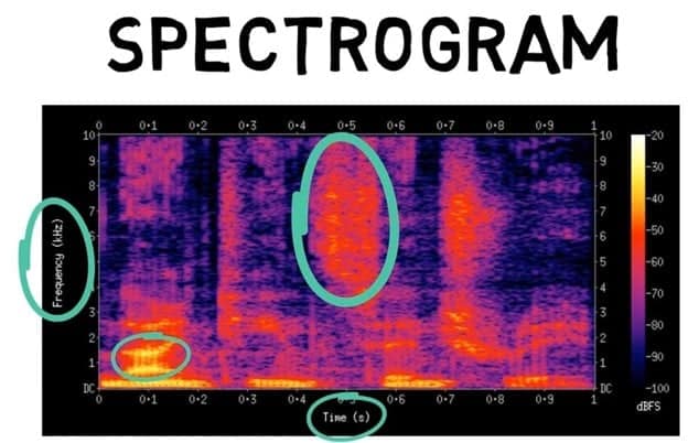

Syntax
There are three categories of syntax – tokenization, stemming, and lemmatization. Tokenization can be split into a further two categories, sentence tokenization, and word tokenization. Sentence tokenization refers to splitting a paragraph into distinct sentences, while word tokenization is separating a sentence into distinct words. This allows the computer to learn the potential meanings and purpose of each unique word.
Stemming refers to the process of reducing a word to its stem or root. It does this by chopping off universal prefixes and suffixes. Stemming is a powerful technique, but is solely based on common prefixes and suffixes. It sometimes cuts necessary components and changes the meaning of the original word.
Lemmatization helps solve this problem. Instead of chopping up beginnings and endings, lemmatization reduces a word to its root form by analyzing the word morphologically. For example, “Am”, “Are”, and “Is”, are root forms of the word “Be”. This can be observed through lemmatization. Stemming would not be able to figure this out since chopping off any letters would not output the word “Be”.
Semantics
Semantics can be broadly categorized into Named Entity Recognition and Natural Language Generation. Named Entity Recognition allows the computer to categorize specific words in a sentence. This is helpful for a word such as “Google” which can be referred to as an organization or a verb. Natural Language Generation is a process through which a machine produces natural human language. It uses math formulas and numerical information to extract patterns and data from a given database and output understandable human language text.
Natural language processing enables a machine to take what you are saying, make sense out of it and formulate a statement of its own to respond to you.
What Is Text to Speech?
What is text to speech? Text to speech software takes the written text and transforms it into speech. There are hundreds of text to speech online applications and numerous text to speech free downloads are available. This technology offers a ton of benefits for people who prefer listening to reading. It is also great for people who want to listen to a piece of text as they perform another task. For example, you can listen to the audio of a book while driving.
Text to speech is also one of the ways that visually impaired individuals consume content. It is known to enhance literacy skills, improve reading comprehension, accuracy, and the ability to recall information. Text to speech can improve word recognition skills and increases pronunciation capabilities.
Many applications can convert text to speech. Google Text-to-Speech is one such tool that enables applications to read out the text on your device’s screen.
Text to speech should not be confused with speech to text. The latter refers to speech recognition where a computer uses your voice input to execute commands. Another potentially confusing term is “voice to text”. What is voice to text? Simply, speech to text can also be referred to as voice to text.
There are also dozens of speech to text individual applications that help with speech to text transcription or to transcribe audio to text. To begin learning how to speech to text, read the documentation in these applications.7700
Advantages of Speech Recognition and Speech to Text
Speech recognition technology has transformed communication and decreased the time it takes to complete tasks. It has also allowed people to use technology in ways that weren’t previously possible. The following are some benefits of speech recognition and benefits of voice recognition.
Helping Disabled Persons
 The most obvious benefit is that speech recognition technology has made it possible for people with disabilities to type and operate computers using their voices as input. Before this technology, many people with certain physical impairments could not use computers effectively, if at all. Speech recognition has brought equity to these people and allowed them to participate in our highly technological society.
Spelling
Using advanced algorithms and natural language processing, speech recognition applications ensure we always use the correct spelling and use words appropriately. Voice recognition has made it possible to write with precision and clarity. This saves lots of time, especially at the workplace.
Enhanced Speed
For people lacking typing skills or are slow typers, voice recognition is a game-changer. Long hours spent typing is also known to cause musculoskeletal health conditions. Speech recognition is, therefore, a safer and faster alternative to getting your thoughts down in print.
Specialization
Speech recognition is also revolutionizing many industries. For example, in the field of medicine, doctors can now add medical notes directly into a patient’s files without having to type or write anything down. They simply speak into a voice recorder and the patient’s Electronic Health Record is automatically updated. This has allowed doctors to spend more time providing treatment and saving lives.
History of Speech Recognition
 In 1791, the first acoustic mechanical speech machine was built by Wolfgang Von Kempelen. It consisted of bellows, a reed and a synthetic mouth made of rubber. With a skilled user, this machine could produce full sentences in English, French, and Italian.
After Kempelen’s device there was a lull in inventions for over a century, until, in 1922, a device known as Radio Rex was invented. This was the first machine capable of recognizing speech. It was a toy dog controlled by a spring and mounted on an electromagnet. The electromagnet was interrupted when there was an acoustic signal of 500 hertz. So, if someone said the word “rex” the dog would pop-up since the word “rex” is about 500 hertz.
In 1952, we had the Audrey system built by Bell Labs. This device could recognize only ten digits.
Next came IBM Shoebox – released to the public in 1962 – which could understand 16 words, the digits 0 to 9, and perform mathematical calculations. This early computer was developed 20 years before the development of the IBM personal computer in 1981.
In 1962, the IBM 704 was invented. This was the first machine that could sing a song – ‘Daisy Bell’.
By the 1970s, machines were able to recognize about 1,000 words. One such tool, named Harpy, was developed at the Carnegie Mellon University in Pennsylvania with the aid of the US Department of Defense.
About ten years later, the same group of scientists developed a system that could not only analyze individual words but entire word sequences. Among the earliest virtual assistants that applied this technology were automated attendants – the canned automated voices we still hear when we dial a customer service number.
In the 1990s, digital speech recognition was a new feature of the personal computer with the likes of Microsoft, IBM, Philips, and Lernout and Hauspie competing for customers. The latter was a Belgian-based speech recognition company that went bankrupt in 2001.
The launch of the first smartphone, the IBM Simon in 1994, laid the foundation for smart virtual assistants as we know them today. The history of voice recognition, where computers could recognize particular speakers, can be traced to this point.
Siri on the iPhone 4S was the first modern incarnation. Google Now arrived a year after Siri, bringing voice recognition to Android. Today, voice assistants are everywhere.
Speech Recognition Applications
There are numerous speech recognition applications today. These are transforming human interaction with devices, cars, homes, and work.
Speech recognition voice assistants have become a ubiquitous part of our lives.
They help us complete basic tasks and respond to our queries. Conventional digital assistants can access information from massive databases. They also rely on deep learning speech recognition and machine learning speech recognition technology to solve problems in real-time, enhance the user experience, and boost productivity.
Popular speech recognition applications include:
Apple Siri
Siri stands for Speech Interpretation and Recognition Interface. The application is invoked by saying the phrase “Hey, Siri”. Siri-enabled iOS apps have specific functions, such as messaging, note-taking, scheduling, etc.
Google Assistant
Google Assistant is an Android speech recognition application. It ships as a standard feature on all Android devices and is invoked by the phrase “Ok, Google”.
Microsoft Cortana
Cortana is a Microsoft application and was named after the AI character from Halo Games. It was created for Windows Phone 8.1 and now comes as standard on all applications running on the Windows operating system. Cortana is invoked using the phrase “Hey, Cortana”. Cortana is said to be the most human-like of all speech recognition applications. It has a team of writers, screenwriters, playwrights, novelists, and essayists who are trying to provide more human-like interaction.
Amazon Alexa
Alexa is available on Amazon Echo and Fire TV. Any developer can contribute to the Amazon Skills library and hence assist with further development.
In addition to these well-known applications, there are many more, such as java speech recognition, java voice recognition and other speech to text applications that offer cross-platform support.
Speech to Text Software
Text to speech software refers to computer programs that scan text and then read it aloud using speech synthesis technology.
On the other side of the coin, speech to text software, speech transcription software and voice to text software all refer to any computer program that inputs audio and returns a written transcript. It is the best way to get a fast, affordable, and easy transcript from a voice sample.
There are hundreds of transcription software services online that offer this service and many companies offer a speech to text software free download. But, the best speech to text software must be able to provide an accuracy rate of at least 90% for clean recordings that are not heavily accented. A good speech to text app will also offer transcription for many languages.
Examples of free speech to text software include Google Text to Speech on Google Cloud and Amazon Transcribe. These two are often regarded as the best transcription software due to the generous free tiers they offer. However, usage is only free up to a certain level, after which the customer is billed for additional usage.
However, speech to text apps and voice to text applications, in general, are yet to reach the accuracy levels of human transcription.
Speech to Text Problems
There are many complaints of voice to text not working. In some cases it’s human error, other times it’s technology glitches.
Some of the things you can quickly and easily check:
- Is your microphone plugged in?
- If the microphone has a mute button, has it been pressed?
Once you’ve ruled that out, consider your voice – are you speaking loudly? Clearly? Is there a slight but perceptible pause between words? Are you hoarse or losing your voice?
While the technology is impressive, it is not immune to bugs especially related to variances in how you speak.
The best solution for speech to text problems is to contact the support network for your particular technology.
How Does Speech to Text Software Work?
How does speech recognition work? The speech recognition process involves multiple steps. Speech creates vibrations that are picked up by an analog-to-digital converter (ADC). The ADC samples the sound and takes frequent detailed wave measurements to complete conversion into digital language. The software applies filters to distinguish different frequencies and relevant sounds because not all sound picked up comprises a part of speech.
The sound is then segmented into hundredths or thousandths of seconds and matched to phonemes. Each phoneme is analyzed in relation to other phonemes and then run through complex algorithms to match them to sentences, words, and phrases in a database. The system then picks an output that best represents what the person has said.
How to do speech to text as a user? Simply speak into your device with a speech to text application enabled and watch your spoken words transform into written text.
How Does Voice Recognition Work?
How voice recognition works is that the software is initially “trained” to recognize a particular person’s voice. For example, when you create a new Google account and add it to a new Android device, Google Assistant will prompt you to record your voice by speaking a series of phrases into the microphone. This way, the application learns your accent and is acquainted with your manner of speech.
What Does Voice Recognition Do?
When you speak, the application “listens” and then follows the same process to output text. Voice recognition is more accurate than speech recognition due to the “training” process. With long-term use, voice assistants can feel like a real human assistant.
Voice Recognition Software
Voice recognition has taken years to develop to a point where it is good for mass adoption. Every breakthrough in years past has left a bitter taste in the mouth as users have found it to be clunky. But, voice recognition has finally gained widespread adoption over recent years due to great advancements in technology.
Early voice recognition software had a limited dictionary size and could not differentiate context. Fortunately, by the late 1990s computers had evolved to have lots of storage and processing power, allowing voice recognition software to comprehend more natural speech instead of forcing users to speak slowly and unnaturally.
 Now, technologies like Apple’s Siri and Cortana, a Windows speech recognition application, don’t depend on limited dictionaries or mobile device processors. Instead, they make use of enormous cloud databases that store billions of words, sentences, and phrases. These cloud servers have nimble CPUs to precisely comprehend what you mean. For example, Google speech recognition software can learn from search engine entries and can also discern a variety of accents. So, you can use it whether you are from Texas, New Delhi, or Zanzibar.
But, it goes further than that. When you ask your voice recognition app for a sports score, how does it know to respond with information about your favorite team instead of giving you information about a random sports score? Instead of listening to just one word at a time, it listens to other words as well for context. It then uses probability to determine what you are trying to say. This is a technical process that uses complex mathematical models. Google, for instance, uses an artificial neural network that works like a human brain using digital neurons to learn and understand what humans are saying. This can be seen when Google Assistant changes what it thinks you said in real-time as you continue talking. And, it gets better. Growth in processing power has made real-time translation possible. You can talk to game characters using a virtual reality headset. Tracking emotions – where a computer uses the timing and pitch of your voice to understand how you are feeling – is now also possible. Uptake has even been seen in the Air Force where voice recognition technologies are deployed in fighter aircraft so that pilots can concentrate on the mission objectives instead of fiddling with instruments.
But although voice recognition has come a long way, it has presented several problems that need to be dealt with. Two stand out above the rest:
- Developers need to find ways to filter out background noise so that you still get accurate results even when you are standing on a noisy street.
- The second issue is privacy. Many types of voice recognition software come with deep learning capabilities. They learn user habits and improve their performance. This, combined with cloud processes, can lead to real concerns. For example, a few years ago, Samsung Smart TVs had a privacy policy that suggested the Samsung voice recognition system was able to monitor conversations occurring within close proximity of the TV.
Streaming Speech Recognition
Streaming speech recognition refers to the real-time streaming of audio to a speech-to-text software program. Text recognition happens simultaneously as the speech plays. A good example of this technology is Google speech to text streaming on YouTube. When you enable the closed captions button on live YouTube video, you will see Google speech recognition and Google voice recognition working in real-time.
Microsoft speech recognition also has streaming speech technology as do many speech recognition python applications.
Streaming speech recognition helps save time where you don’t want to have to wait to transcribe the entire audio.
It also helps people with impaired hearing to follow live broadcasts.
Automatic Speech Recognition
ASR (automatic speech recognition) refers to speech recognition programs that analyze audio and convert it to text without human intervention.
There are four key differences between automatic speech transcription and human transcription services.
Cost
Human transcription costs a lot more than automatic speech transcription. Most automated speech recognition services have a free tier in terms of audio minutes or hours. Once these are exhausted, the service is costed on a per-audio-hour or -minute basis.
Time
ASR is also much faster than human speech to text transcriptions. A highly skilled human transcriber can transcribe one hour of audio in 4 to 6 hours, while automatic speech recognition software can get it done in a few minutes.
Quality
While automatic speech transcription is cheaper and faster, it has a much lower level of accuracy. Speech to text software programs needs clear audio to output high accuracy. Unfortunately, most recorded audio is rarely 100% clear. There is background noise, heavy accents, false starts, and stutters. As a result, ASR will rarely deliver 99% accuracy. Professional human transcription, on the other hand, usually can.
Versatility
ASR can only output verbatim transcript whereas a human can offer a wider spectrum of options such as verbatim, intelligent verbatim – where stutters, errors, and false starts are corrected – and even summarized notes.
Text to Speech Conversion
Text to speech (TTS) falls within the broad category of assistive technology that outputs text to audio. With the tap of a finger or a mouse click, text to speech programs can take speech and convert it into audio.
Text to speech conversion is useful for people who struggle with reading. It also assists with writing, editing, and improving focus.
Today, just about every digital device has a text to voice converter. All manner of text files can be read aloud, including webpages by activating inbuilt website tools available on-screen, or by using browser plugins and extensions.
The voice is generated by a computer using speech synthesis technology. It can be slowed down or sped up depending on user preferences. The voice quality also varies with each application. Some applications are said to sound more human than others.
There are five main speech to text tools:
- Built-in text-to-speech: Many devices come with built-in TTS tools. Your standard computer, mobile phone, or tablet most likely has one. These can be used without the need for special applications or software.
- Web-based tools: Some websites come with built-in TTS tools. Otherwise, the functionality can be added using a plugin. For example, numerous WordPress plugins let you add a text to voice converter to your website. Website visitors then click on an icon to hear the text read aloud.
- Text-to-speech apps: These are downloadable apps available on The Play Store for Android and App Store for iOS, usually with a rich variety of features.
- Chrome extensions: Chrome comes with several free extensions that read out text aloud. They can be found at the Chrome Web Store.
- Text-to-speech software programs: There are also several stand-alone text-to-speech programs compatible with various operating systems.
Ways to Convert Speech to Text
Let’s examine several ways to convert conversation to text.
Google provides several options to transcribe audio to text free of charge.
The first is through Google Docs Voice to Text, a free audio to text converter. This works with Chrome browsers on Google Docs or Google Slides.
The Google Translate app also converts voice to text. When you open the page, there is a small microphone that allows you to speak into the device. The words are captured, converted to text, and translated to your desired language.
You can also upload an audio file to Google text to speech on Google cloud and create a transcription project. Once the file is transcribed, you can download it or share it online.
Speech to text Android functionality is also a standard feature via Google Assistant.
Windows Dictation
This functionality was built into Windows 10 by Microsoft. You can type a document using your voice by placing your cursor at the location of an MS Word document and speaking into a microphone.
Apple Dictation
Just like in Windows, Apple dictation is a speech to text converter built into a Mac. You simply place your cursor wherever you want the text to appear and speak into the microphone.
Amazon Transcribe
Amazon Transcribe works as an audio file to text converter. You simply upload an audio file to your S3 container and then create a transcription job. Once the file is transcribed you get a notification and can download it or share it.
Other Applications
The top three are the most common due to the sheer number of devices that ship with them as standard features. However, there are hundreds of applications for converting voice to text. They range from simple to advanced tools with a wide range of features.
Summary:
How Does Speech to Text Software Work?
How does speech recognition work? The speech recognition process involves multiple steps. Speech creates vibrations that are picked up by an analog-to-digital converter (ADC). The ADC samples the sound and takes frequent detailed wave measurements to complete conversion into digital language. The software applies filters to distinguish different frequencies and relevant sounds because not all sound picked up comprises a part of speech. The sound is then segmented into hundredths or thousandths of seconds and matched to phonemes. Each phoneme is analyzed in relation to other phonemes and then run through complex algorithms to match them to sentences, words, and phrases in a database. The system then picks an output that best represents what the person has said. How to do speech to text as a user? Simply speak into your device with a speech to text application enabled and watch your spoken words transform into written text.