Word search end of cell

When Peter wants to find a word at the end of a paragraph, he searches for XXX^p and replaces it with YYY^p. This doesn’t, however, find words at the very end of table cells. He wonders how he can search and replace the words at the end of table cells and if there is a special code similar to ^p.

There is no special code similar to ^p (end of paragraph) to indicate the end of a cell. There is a trick you can try, however, that works well for many people.

First, create a unique paragraph style that you will use only for the contents of the cells in your table. Make sure you apply this style to all of the cells within the table. Next, use Find and Replace to search for the style. In the Replace With box, enter the code ^& followed by what you want to add to the end of the cell. Then, step through all occurrences and do your replacements, as desired. The ^& code specifies that you want to replace what you found (the text in the cells formatted with the unique style) with what you actually found.

If you want to replace a specific word in the table cells (XXX) with something new (YYY), you can follow the same steps as above, simply search for any occurrences of XXX using the unique table-cell style and replace it with YYY. You’ll still want to step through the matches and determine if the replacement should be made on a case-by-case basis, but you will be able to make the changes in your table much quicker.

Author Bio

With more than 50 non-fiction books and numerous magazine articles to his credit, Allen Wyatt is an internationally recognized author. He is president of Sharon Parq Associates, a computer and publishing services company. Learn more about Allen…

1. 06-20-2014, 07:19 AM

   
   

   #1

   

   
   Registered User
   

   

   ---

   Word macro to find end of cell mark
   

   Hi Everyone,

   I have a big word table with 3 columns and many rows. I want to find the end of cell mark to do some checks, but it seems there is no simple way to find end of cell mark in Word and I need a macro for that.

   In the first column and last column, I want to highlight in blue color space or spaces or paragraph marks just before the end of each cell.
   Similarly in the second column, I want to highlight in blue when there are 2 paragraph marks or when there are no paragraph marks or when there are space/spaces symbols just before the end of each cell. Kindly help me write a macro.

   Pls note there would be normal text other than this table in the word document and these checks should be done only in the table.

   Thank you for your help!

   ---

2. 06-20-2014, 09:11 PM

   
   

   #2

   Re: Word macro to find end of cell mark
   

   The end-of-cell mark is always the last character in a cell. Your column-2 criteria are quite ambiguous, especially as to what you might mean by ‘symbols’ and what happens if there are no paragraph breaks before the end-of-cell mark.

   Try:

   Cheers,
   Paul Edstein
   [Fmr MS MVP — Word]

   ---

3. 06-20-2014, 11:29 PM

   
   

   #3

   

   
   Registered User
   

   

   ---

   Re: Word macro to find end of cell mark
   

   Hi,

   Thank you very much for the macro! Sorry for not being clear. If there are no paragraph marks I just want to color the last word. I have used the wrong word symbols, it is just spaces. Please explain what «While .Characters.First.Previous Like «[ ]»» means and pls tell how to color the last word in 2 column when there are no paragraph mark before the end of cell mark.

   Thanks once again!

   ---

4. 06-20-2014, 11:41 PM

   
   

   #4

   Re: Word macro to find end of cell mark
   

   The «While .Characters.First.Previous Like «[ ]»» expression is part of a While … Wend loop that keeps extending the range forward for each space character that precedes the current range.

   To colour the last word when not followed by a paragraph break, change:
   If Len(.Text) <> 1 Then .Font.ColorIndex = wdBlue
   to:
   If Len(.Text) > 1 Then .Font.ColorIndex = wdBlue
   If Len(.Text) = 0 Then .Characters.First.Previous.Words.First.Font.ColorIndex = wdBlue

   ---

5. 06-21-2014, 03:40 AM

   
   

   #5

   

   
   Registered User
   

   

   ---

   Re: Word macro to find end of cell mark
   

   Thank you! This is working like a charm, but when we change the font color it is not very obvious. Please tell how to highlight in blue.

   ---

6. 06-21-2014, 05:37 AM

   
   

   #6

   Re: Word macro to find end of cell mark
   

   You can change any of the ‘.Font.ColorIndex’ references to ‘.HighlightColorIndex’.
   For example, instead of using:
   .Font.ColorIndex = wdBlue
   you might use:
   .HighlightColorIndex = wdBrightGreen

   ---

7. 06-21-2014, 08:26 AM

   
   

   #7

   

   
   Registered User
   

   

   ---

   Re: Word macro to find end of cell mark
   

   Thank you! It is working great!

   ---

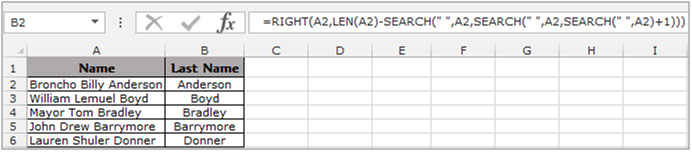
To extract the last word from the text in a cell we will use the “RIGHT” function with “SEARCH” & “LEN” function in Microsoft Excel 2010.

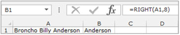
RIGHT:Return the last character(s) in a text string based on the number of characters specified.

Syntax of “RIGHT” function: =RIGHT (text, [num_chars])

Example:Cell A1 contains the text “Broncho Billy Anderson”

=RIGHT (A1, 8), function will return “Anderson”

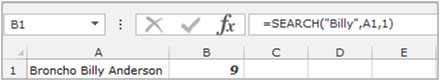
SEARCH:The SEARCH function returns the starting position of a text string which it locates from within the text string.

Syntax of “SEARCH” function: =SEARCH (find_text,within_text,[start_num])

Example:Cell A2 is containing the text “Broncho Billy Anderson”

=SEARCH («Billy», A1, 1), function will return 9

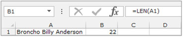
LEN:Returns the number of characters in a text string.

Syntax of “LEN” function: =LEN (text)

Example:Cell A1 contains the text “Broncho Billy Anderson”
=LEN (A1), function will return 22

Understanding the process of Extracting Characters from Text Using Text Formulas

Example 1: We have a list of Names in Column “A” and we need to pick the Last name from the list. We will use the “LEFT” function along with the “SEARCH” function.

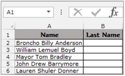
To separate the last word from a cell follow below steps:-

• Select the Cell B2, write the formula =RIGHT(A2,LEN(A2)-SEARCH(» «,A2,SEARCH(» «,A2,SEARCH(» «,A2)+1))) function will return the last name from the cell A2.

  To Copy the formula to all the cells press key “CTRL + C” and select the cell B3 to B6 and press key “CTRL + V” on your keyboard.

• To convert the formulae into values, select the function range B2:B6, and “COPY” by pressing the key “CTRL + C”, right click of the mouse select “Paste Special”.
• The Paste Special dialog box will appear. Click on “Values” then click on ok to convert the formula into values.

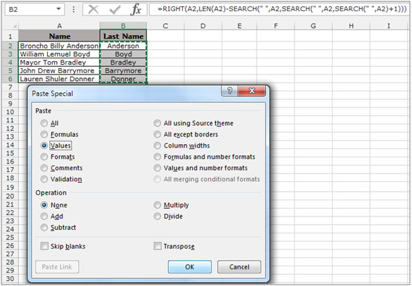
This is how we can extract the last word in a cell into another cell.

In Excel you may need to lookup just part of the text in a cell. For example, if you have a cell that contains a transaction description and within that description there is a product name.

You want to lookup the price of that product from a table. Let’s look at three possibilities:

1. 1. When the product name is just randomly placed within the lookup text: “Sold WHEEL to John’s Motors Ltd”
   2. As 1. above but there are always defined characters before and after the product name: “Sold –WHEEL– to John’s Motors Ltd”
   3. The product name is always in the same part of the string: “AA2 WHL Sold – JM1″

Obviously the third possibility in the list is the easiest to solve in Excel so lets begin there.

Lookup Part of Text in Cell: Consistent Start and End Points

The VLOOKUP (or HLOOKUP) function has the following arguments: LOOKUP VALUE, TABLE, COLUMNS INDEX NUMBER, EXACT/NON-EXACT MATCH. As the LOOKUP VALUE is only part of the cell, we need to consider how we can extract the text we want from the cell.

Check FIG(a1) for the LOOKUP VALUE sources and TABLE ARRAY.

Find the LOOKUP VALUE Part of the Cell

Since in this case the start point in each source cell is consistently character 5 and the length of the LOOKUP VALUE will always be 3 characters (such as “WHL” in cell D8), we can use the MID function to extract the LOOKUP VALUE. The MID function just needs the TEXT, START CHARACTER NUMBER and NUMBER OF CHARACTERS.

In our example lets start by inputting the MID function in cell F8. You can see the result in FIG(a2).

The result of this we now just need to use in our VLOOKUP formula. The LOOKUP TABLE being in range $H$8:$I$10, COLUMN INDEX NUMBER is 2 (the second column in the table) and in this case we only want to return exact matches so the final argument will be ‘FALSE’.

Finalize the Formula to Lookup Part of the Cell

Putting that formula together in our cell F8 is:

=VLOOKUP(MID($D8, 5, 3), $H$8:$I$10, 2, FALSE)

Copying down that formula next to our transactions completes the lookup of prices FIG(a3).

Moving on to our next scenario.

Lookup Part of Text: Using a Consistent Character as Separator

In this case we will use the separator ‘-‘ to define the start and end of the LOOKUP VALUES in the source cells. This method works as long as the separator character is only used to identify the Product Name. If appears elsewhere in the text then you can proceed to scenario 3 which can handle the LOOKUP VALUE anywhere in the cell.

Use the Dashes to Separate the LOOKUP VALUE

You can see in FIG(b1) that if we find the dashes ‘-‘ we will be able to extract the needed text using the MID function. To do this we will need to know the starting character for “Wheel” and the number of characters in “Wheel”. We will use the FIND function to identify the placement of our separators and do these calculations.

FIND first separator

In FIG(b2) you can see the make up of the FIND function to locate the start of “Wheel”. The FIND function has the following arguments: FIND TEXT, WITHIN TEXT and an optional CHARACTER START NUMBER. This third optional argument is useful when you are looking for the second or subsequent separator. We will use it later but for now we can ignore it.

So putting our FIND function in cell F17. [FIG(b2)] you can see it has returned the placement of the of the first dash.

=FIND(“-“,   $D17)

FIND second separator

Now, lets find the second separator so we can find the end of our LOOKUP VALUE. We are going to do this by doing another FIND formula. This time though we will need to use the START NUMBER to make sure we skip past the separator we’ve already discovered.

In FIG(b3) you can see the first two arguments of the second FIND are exactly the same. But to skip over the first separator we need to get the number for this from cell F17 (+1 to jump past it).

=FIND(“-“,   $D17,  F17+1)

Use MID Function to Get the LOOKUP VALUE

Now we have those results we can put together a MID function (as used in the first scenario).

FIG(b4). The first argument of the MID function is just our transaction description. Second is the start point which is our first FIND function. Next we need the number of characters to extract. We can calculate this as our second FIND result less the first. You can see we have extracted the LOOKUP VALUE.

=MID($D17,   F17+1,   G17-1-F17)

Before going on to the last step lets combine our functions. You can do this by editing the cell with the first FIND and copying everything after the “=”. Leave this cell then edit our MID function in cell …. highlight the reference to cell …. and paste. Repeat this for the second FIND function. Great, that’s our MID function complete.

You should end up with this:

=MID($D17,  FIND(“-“,   $D17)+1,  FIND(“-“, $D17,FIND(“-“,$D17)+1)   -1    -FIND(“-“,   $D17))

VLOOKUP part of text

Finally we can do our VLOOKUP using this MID function as the LOOKUP VALUE. In FIG(b6) you can see we’ve referenced this cell, input our table, selected the second column and indicated we want exact match (FALSE).

=VLOOKUP(F17,   $J$17:$K$19,   2,   FALSE)

We will just replace the reference to cell F17 with the formula in that cell. Copy that down and we’re done FIG(b7).

=VLOOKUP(MID($D17,  FIND(“-“,   $D17)+1,  FIND(“-“, $D17,FIND(“-“,$D17)+1)   -1    -FIND(“-“,   $D17)),   $J$17:$K$19,   2,   FALSE)

There are a few steps there but hopefully the logic makes sense. Now lets move on to the final scenario where you can lookup pretty much any of the possible Product Names wherever they appear in our source text.

Lookup Part of Text: Randomly Placed Text in Cell

In order to lookup part of text in a cell that is randomly placed; we are going to need something other than the VLOOKUP function. Instead we are going to create a fairly complicated ARRAY FORMULA that uses INDEX, MATCH, ISERROR and FIND. If any of these functions are unfamiliar, don’t worry. Just follow it through. Once you’ve built the array formula hopefully you can understand the logic in those functions.

The Logic In This Solution

Lets consider the logic of this approach to look up part of the cell. We are going to use what I’ll call a reverse lookup. I.e. we’re going to try each of the items in column H (the first column of our lookup table) to see if the text in those cells is anywhere in our source cell (the descriptions in column D). Once we’ve found one that matches, we’ll look down the corresponding data in column I and get the result.

Ok, lets begin by seeing if we can find an item in column H that is in our lookup source cells.

ARRAY Formulas

An ARRAY formula allows us to use an array of values (compared with a standard equivalent formula where we’d just be able to use a single value).

You may be aware that the FIND function returns an error if it can’t locate the searched text. E.g. =FIND(“C”,  “ABD”) returns an error.

So as part of an ARRAY formula, =FIND({“A”,”B”,”C”,”D”},     “SAMPLE TEXT”) would return {2,ERROR,ERROR,ERROR}.

Applying that to our data would result be: =FIND({“Chrome Wheel”,”Bearings”,”Wheel”,”Tyre”},     “Sold Wheel to John’s Motors Ltd”) and return {ERROR,ERROR,6,ERROR}

Hopefully you can see this may be useful. If we can identify where the first non-error occurs we can find the position in the table for our result.

MATCH Function In ARRAY FORMULA

To find the non-error we can use MATCH function to look through the results of the FIND array.

Before we do that lets use the ISERROR function to convert {ERROR,ERROR,6,ERROR} to {TRUE,TRUE,FALSE,TRUE}.

Now instead of numbers we have FALSE to look for.

The FALSE results are the nuggets we’re looking for.

To find the placement of the FALSE we can use the MATCH function. So “=MATCH(FALSE,  {TRUE,TRUE,FALSE,TRUE},   0)” in an ARRAY formula is going to return 3.

Lets try inputting the ARRAY FORMULA so far to make sure it is working as expected. See FIG(c1) for the formula.

{=MATCH(FALSE, ISERROR(SEARCH($H$31:$H$34, $D31)), 0)}

To enter an ARRAY formula, press SHIFT+CTRL+ENTER (rather than just ENTER). This tells Excel you want an array formula. You don’t type the leading and ending {}. Hitting SHIFT+CTRL+ENTER will put these in. Make sure you check these are shown once you’ve done the SHIFT+CTRL+ENTER.

You can see this is returning 3 which is the correct row in our table for “Wheel”.

Complete the Lookup with INDEX Function

We’re almost done with the tutorial. All we need to do now is use this result in an INDEX function.

If you’re not familiar with the INDEX function the arguments are: ARRAY, ROW NUMBER, and optional COLUMN number. We can complete this with one column so the final argument won’t be needed for this example.

So our INDEX function looks at the lookup table and identify the cell you want from the table by identifying which row to select from it.

Putting this altogether you can see the result in FIG(c2). So we’re looking down our table in column I by the number of rows identified by the MATCH function.

{=INDEX($I$31:$I$34, MATCH(FALSE, ISERROR(SEARCH($H$31:$H$34, $D31)), 0))}

We can copy this down and we have results for all our lookups.

What To Watch Out For

1. The FIND function is case sensitive. To remove this sensitivity, you can either keep the data in column H in upper case and amend the formula to: INDEX($I$31:$I$34, MATCH(FALSE, ISERROR(FIND($H$31:$H$34, UPPER($D31))), 0)). Fig(c3). Or you can replace FIND with SEARCH. The SEARCH function is not case sensitive.
2. You need to think about the order of your data in the lookup table. As Excel is going to run down the data in column H it will find the first match. A cell with the words “….CHROME WHEEL…” could match to both “WHEEL” and “CHROME WHEEL”. So in this case you’d want to ensure “CHROME WHEEL” was above “WHEEL” in your table. You

   

   Fig(c3)

   may resolve this problem by sorting your list by length of “Product Name”.

Hopefully you find this functionality useful. If you have any questions or comments please post them below.

You can also learn how to create a hyperlink to VLOOKUP or SUMIF results.

And if you’re looking to include wildcards in the ‘lookup what’ then check out these wildcard examples.