Word functions in excel

To get detailed information about a function, click its name in the first column.

Note: Version markers indicate the version of Excel a function was introduced. These functions aren’t available in earlier versions. For example, a version marker of 2013 indicates that this function is available in Excel 2013 and all later versions.

Function	Description
ARRAYTOTEXT function	Returns an array of text values from any specified range
ASC function	Changes full-width (double-byte) English letters or katakana within a character string to half-width (single-byte) characters
BAHTTEXT function	Converts a number to text, using the ß (baht) currency format
CHAR function	Returns the character specified by the code number
CLEAN function	Removes all nonprintable characters from text
CODE function	Returns a numeric code for the first character in a text string
CONCAT function	Combines the text from multiple ranges and/or strings, but it doesn’t provide the delimiter or IgnoreEmpty arguments.
CONCATENATE function	Joins several text items into one text item
DBCS function	Changes half-width (single-byte) English letters or katakana within a character string to full-width (double-byte) characters
DOLLAR function	Converts a number to text, using the $ (dollar) currency format
EXACT function	Checks to see if two text values are identical
FIND, FINDB functions	Finds one text value within another (case-sensitive)
FIXED function	Formats a number as text with a fixed number of decimals
LEFT, LEFTB functions	Returns the leftmost characters from a text value
LEN, LENB functions	Returns the number of characters in a text string
LOWER function	Converts text to lowercase
MID, MIDB functions	Returns a specific number of characters from a text string starting at the position you specify
NUMBERVALUE function	Converts text to number in a locale-independent manner
PHONETIC function	Extracts the phonetic (furigana) characters from a text string
PROPER function	Capitalizes the first letter in each word of a text value
REPLACE, REPLACEB functions	Replaces characters within text
REPT function	Repeats text a given number of times
RIGHT, RIGHTB functions	Returns the rightmost characters from a text value
SEARCH, SEARCHB functions	Finds one text value within another (not case-sensitive)
SUBSTITUTE function	Substitutes new text for old text in a text string
T function	Converts its arguments to text
TEXT function	Formats a number and converts it to text
TEXTAFTER function	Returns text that occurs after given character or string
TEXTBEFORE function	Returns text that occurs before a given character or string
TEXTJOIN function	Combines the text from multiple ranges and/or strings
TEXTSPLIT function	Splits text strings by using column and row delimiters
TRIM function	Removes spaces from text
UNICHAR function	Returns the Unicode character that is references by the given numeric value
UNICODE function	Returns the number (code point) that corresponds to the first character of the text
UPPER function	Converts text to uppercase
VALUE function	Converts a text argument to a number
VALUETOTEXT function	Returns text from any specified value

Important: The calculated results of formulas and some Excel worksheet functions may differ slightly between a Windows PC using x86 or x86-64 architecture and a Windows RT PC using ARM architecture. Learn more about the differences.

See Also

Excel functions (by category)

Excel functions (alphabetical)

For the convenience of working with text in Excel, there are text functions. They make it easy to process hundreds of lines at once. Let’s consider some of them on examples.



Examples with TEXT function in Excel

This function converts numbers to string in Excel. Syntax: value (numeric or reference to a cell with a formula that gives a number as a result); Format (to display the number in the form of text).

The most useful feature of the TEXT function is the formatting of numeric data for merging with text data. Excel «doesn’t understand» how to display numbers without using the function. The program just converts them to a basic format.

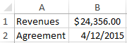
Let’s see an example. Let’s say you need to combine text in string with numeric values:

Using an ampersand without a function TEXT produces an inadequate result:

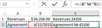
Excel returned the sequence number for the date and the general format instead of the monetary. The TEXT function is used to avoid this. It formats the values according to the user’s request.

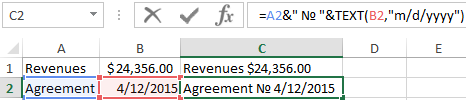
The formula «for a date» now looks like this:

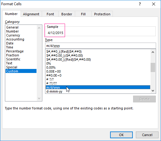
The second argument to the function is the format. Where to take the format line? Right-click on the cell with the value. Click on «Format Cells». In the opened window select «Custom». Copy the required «Type:» in the line. We paste the copied value in the formula.

Let’s consider another example where this function can be useful. Add zeros at the beginning of the number. Excel will delete them if you enter it manually. Therefore, we introduce the formula:

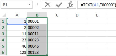
If you want to return the old numeric values (without zeros), then use the «—» operator:

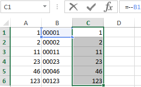
Note that the values are now displayed in numerical format.



Text splitting function in Excel

Individual functions and their combinations allow you to distribute words from one cell to separate cells:

• LEFT (Text, number of characters) displays the specified number of characters from the beginning of the cell;
• RIGHT (Text, number of characters) returns a specified number of characters from the end of the cell;
• SEARCH (Search text, range to search, start position) shows the position of the first occurrence of the searched character or line while viewing from left to right.

The line takes into account the position of each character when dividing the text. Spaces show the beginning or the end of the name you are looking for.

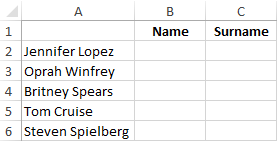
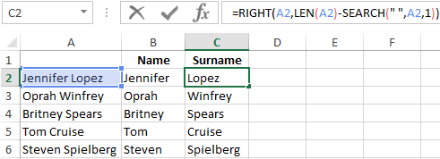
We will split the name, surname and patronymic name into different columns using the functions.

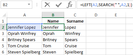
The first line contains only the first and last names separated by a space. Formula for retrieving the name:

The function SEARCH is used to determine the second argument of the LEFT function (the number of characters). It finds a space in cell A2 starting from the left.

For a name, we use the same formula:

Excel determines the number of characters for the RIGHT function using the SEARCH function. The LEN function «counts» the total length of the text. Then the number of characters up to the first space (found by SEARCH) is subtracted.

The formula for extracting the surname:

Next formulas for extracting the surname is a bit different:

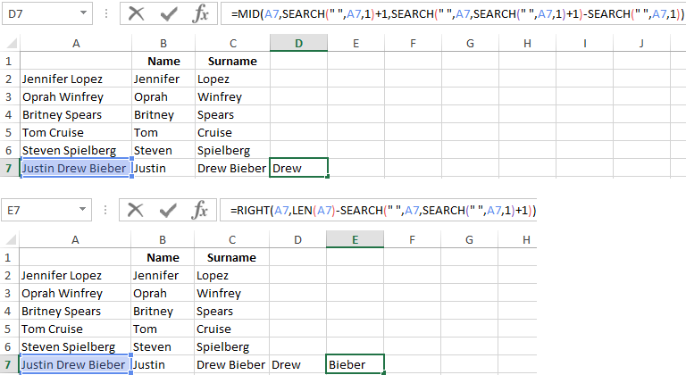
These are five signs on the right. Embedded SEARCH functions search for the second and third spaces in a string. SEARCH («»;A7;1) finds the first space on the left (before the patronymic name). Add one (+1) to the result. We get the position with which we will search for the second space.

Part of the formula SEARCH(» «;A7;SEARCH(» «;A7;1)+1) finds the second space. This will be the final position of the patronymic.

Then the number of characters from the beginning of the line to the second space is subtracted from the total length of the line. The result is the number of characters to the right that you need to return.

Function for merging text in Excel

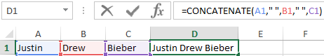
Use the ampersand (&) operator or the CONCATENATE function to combine values from several cells into one line.

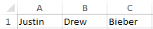
For example, the values are located in different columns (cells):

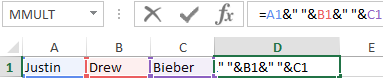
Put the cursor in the cell where the combined three values will be. Enter «=». Select the first cell and click on the keyboard «&» sign. Then enter the space character enclosed in quotation marks (» «). Enter again «&». Therefore, sequentially connect cells with symbols and spaces.

We get the combined values in one cell:

Using the CONCATENATE function:

You can add any sign or string to the final expression using quotation marks in the formula.

Text SEARCH function in Excel

The SEARCH function returns the starting position of the searched text (not case sensitive). For example:

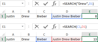
The SEARCH returned to position 8 because the word «Drew» begins with the tenth character in the line. Where can this be useful?

The SEARCH function determines the position of the character in the string line. And the MID function returns symbols values (see the example above). Alternatively, you can replace the found text with the REPLACE.

Download example TEXT functions

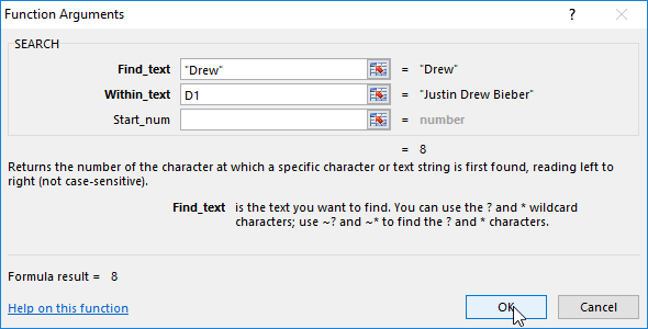
The syntax of the SEARCH function:

• «Find_text» is what you need to find;
• «Withing_text» is where to look;
• «Start_num» is from which position to start searching (by default it is 1).

Use the FIND if you need to take into account the case (lower and upper).

In Excel, there are multiple string (text) functions that can help you to deal with textual data. These functions can help you to change a text, change the case, find a string, count the length of the string, etc. In this post, we have covered top text functions. (Sample Files)

1. LEN Function

LEN function returns the count of characters in the value. In simple words, with the LEN function, you can count how many characters are there in value. You can refer to a cell or insert the value in the function directly.

Syntax

LEN(text)

Arguments

• text: A string for which you want to count the characters.

Example

In the below example, we have used the LEN to count letters in a cell. “Hello, World” has 10 characters with a space between and we have got 11 in the result.

In the below example, “22-Jan-2016” has 11 characters, but LEN returns 5.

The reason behind it is that the LEN function counts the characters in the value of a cell and is not concerned with formatting.

Related: How to COUNT Words in Excel

2. FIND Function

FIND function returns a number which is the starting position of a substring in a string. In simple words, by using the find function you can find (case sensitive) a string’s starting position from another string.

Syntax

FIND(find_text,within_text,[start_num])

Arguments

• find_text: The text which you want to find from another text.
• within_text: The text from which you want to locate the text.
• [start_num]: The number represents the starting position of the search.

Example

In the below example, we have used the FIND to locate the “:” and then with the help of MID and LEN, we have extracted the name from the cell.

3. SEARCH Function

SEARCH function returns a number which is the starting position of a substring in a string. In simple words, with the SEARCH function, you can search (non-case sensitive) for a text string’s starting position from another string.

Syntax

SEARCH(find_text,within_text,[start_num])

Arguments

• find_text: A text which you want to find from another text.
• within_text: A text from which you want to locate the text. You can refer to a cell, or you can input a text in your function.

Example

In the below example, we are searching for the alphabet “P” and we have specified start_num as 1 to start our search. Our formula returns 1 as the position of the text.

But, if you look at the word, we also have a “P” in the 6th position. That means the SEARCH function can only return the position of the first occurrence of a text, or if you specify the start position accordingly.

4. LEFT Function

LEFT Functions return sequential characters from a string starting from the left side (starting). In simple words, with the LEFT function, you can extract characters from a string from its left side.

Syntax

LEFT(text,num_chars)

Arguments

• text: A text or number from which you want to extract characters.
• [num_char]: The number of characters you want to extract.

Example

In the below example, we have extracted the first five digits from a text string using LEFT by specifying the number of characters to extract.

In the below example, we have used LEN and FIND along with the LEFT to create a formula that extracts the name from the cell.

5. RIGHT Function

The RIGHT function returns sequential characters from a string starting from the right side (ending). In simple words, with the RIGHT function, you can extract characters from a string from its left side.

Syntax

RIGHT(text,num_chars)

Arguments

• text: A text or number from which you want to extract characters.
• [num_char]: A number of characters you want to extract.

Example

In the below example, we have extracted 6 characters using the right function. If you know, how many characters you need to extract from the string, you can simply extract them by using a number.

Now, if you look at the below example, where we have to extract the last name from the cell, but we are not confirmed about the number of characters in the last name.

So, we are using LEN and FIND to get the name. Let me show you how we have done this.

First of all, we have used the LEN to get the length of that entire text string, then we used the FIND to get the position number of space between first and last names. And in the end, we have used both the figures to get the last name.

Arguments

• value1: A cell reference, an array, or a number that is directly entered into the function.
• [value2]: A cell reference, an array, or a number that is directly entered into the function.

6. MID Function

MID returns a substring from a string using a specific position and number of characters. In simple words, with MID, you can extract a substring from a string by specifying the starting character and number of characters you want to extract.

Syntax

MID(text,start_num,num_chars)

Arguments

• text: A text or a number from which you want to extract characters.
• start_char: A number for the position of the character from where you want to extract characters.
• num_chars: The number of characters you want to extract from the start_char.

Example

In the below example, we have used different values:

• From the 6th character to the next 6 characters.
• From the 6th character to the next 10 characters.
• We have used starting a character in negative and it has returned an error.
• By using 0 for the number of characters to extract and it has returned a blank.
• With a negative number for the number of characters to extract and it has returned an error.
• The starting number is zero and it has returned an error.
• Text string directly into the function.

7. LOWER Function

LOWER returns the string after converting all the letters in small. In simple words, it converts a text string where all the letters you have are in small letters, numbers will stay intact.

Syntax

LOWER(text)

Arguments

• text: The text which you want to convert to the lowercase.

Example

In the below example, we have compared the lower case, upper case, proper case, and sentence case with each other.

A lower case text has all the letters in a small case compared to others.

8. PROPER Function

The PROPER function returns the text string into a proper case. In simple words, with a PROPER function where the first letter of the word is in capital and rest in small (proper case).

Syntax

PROPER(text)

Arguments

• text: The text which you want to convert to the proper case.

Example

In the below example, we have a proper case that has the first letter in the capital case in a word and the rest of the letters are in the lower case compared to the other two cases lowercase and uppercase.

In the below example, we have used the PROPER function to streamline first name and last name into the proper case.

9. UPPER Function

The UPPER function returns the string after converting all the letters in the capital. In simple words, it converts a text string where all the letters you have are in capital form and numbers will stay intact.

Syntax

UPPER(text)

Arguments

• text: The text which you want to convert into uppercase.

Example

In the below example, we have used the UPPER to convert name text to capital letters from the text in which characters are in different cases.

10. REPT Function

REPT function returns a text value several times. In simple words, with the REPT function, you can specify a text, and a number to repeat that text.

Syntax

REPT(value1, [value2], …)

Example

In the below example, we have used different type of text for repetition using REPT. It can repeat any type of text or numbers and even symbols that you specify in function and the main use of the REPT function is for creating in-cell charts.

Excel предлагает большое количество функций, с помощью которых можно обрабатывать текст. Область применения текстовых функций не ограничивается исключительно текстом, они также могут быть использованы с ячейками, содержащими числа. В рамках данного урока мы на примерах рассмотрим 15 наиболее распространенных функций Excel из категории Текстовые.

СЦЕПИТЬ

Для объединения содержимого ячеек в Excel, наряду с оператором конкатенации, можно использовать текстовую функцию СЦЕПИТЬ. Она последовательно объединяет значения указанных ячеек в одной строке.

СТРОЧН

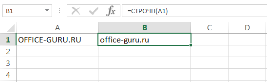
Если в Excel необходимо сделать все буквы строчными, т.е. преобразовать их в нижний регистр, на помощь придет текстовая функция СТРОЧН. Она не заменяет знаки, не являющиеся буквами.

ПРОПИСН

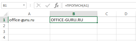
Текстовая функция ПРОПИСН делает все буквы прописными, т.е. преобразует их в верхний регистр. Так же, как и СТРОЧН, не заменяет знаки, не являющиеся буквами.

ПРОПНАЧ

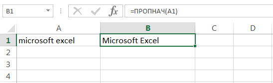
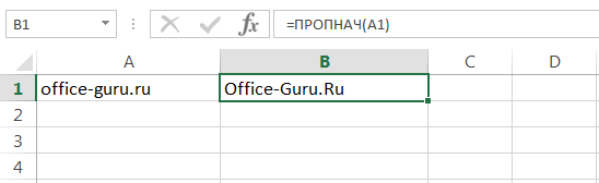
Текстовая функция ПРОПНАЧ делает прописной первую букву каждого слова, а все остальные преобразует в строчные.

Каждая первая буква, которая следует за знаком, отличным от буквы, также преобразуется в верхний регистр.

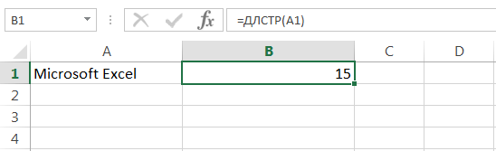
ДЛСТР

В Excel Вы можете подсчитать количество знаков, содержащихся в текстовой строке, для этого воспользуйтесь функцией ДЛСТР. Пробелы учитываются.

ЛЕВСИМВ и ПРАВСИМВ

Текстовые функции ЛЕВСИМВ и ПРАВСИМВ возвращают заданное количество символов, начиная с начала или с конца строки. Пробел считается за символ.

ПСТР

Текстовая функция ПСТР возвращает заданное количество символов, начиная с указанной позиции. Пробел считается за символ.

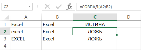
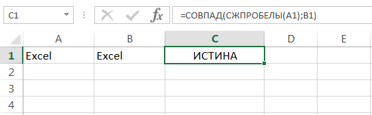
СОВПАД

Функция СОВПАД позволяет сравнить две текстовые строки в Excel. Если они в точности совпадают, то возвращается значение ИСТИНА, в противном случае – ЛОЖЬ. Данная текстовая функция учитывает регистр, но игнорирует различие в форматировании.

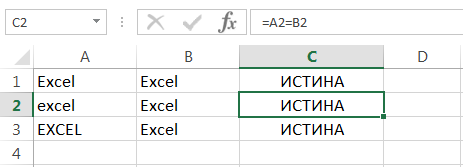
Если регистр для Вас не играет большой роли (так бывает в большинстве случаев), то можно применить формулу, просто проверяющую равенство двух ячеек.

СЖПРОБЕЛЫ

Удаляет из текста все лишние пробелы, кроме одиночных между словами.

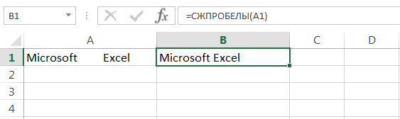
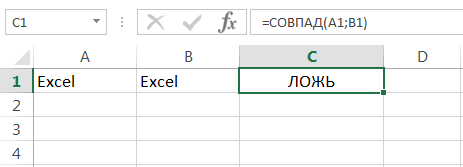
В случаях, когда наличие лишнего пробела в конце или начале строки сложно отследить, данная функция становится просто незаменимой. На рисунке ниже видно, что содержимое ячеек А1 и B1 абсолютно одинаково, но это не так. В ячейке А1 мы намеренно поставили лишний пробел в конце слова Excel. В итоге функция СОВПАД возвратила нам значение ЛОЖЬ.

Применив функцию СЖПРОБЕЛЫ к значению ячейки А1, мы удалим из него все лишние пробелы и получим корректный результат:

Функцию СЖПРОБЕЛЫ полезно применять к данным, которые импортируются в рабочие листы Excel из внешних источников. Такие данные очень часто содержат лишние пробелы и различные непечатаемые символы. Чтобы удалить все непечатаемые символы из текста, необходимо воспользоваться функцией ПЕЧСИМВ.

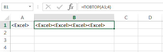
ПОВТОР

Функция ПОВТОР повторяет текстовую строку указанное количество раз. Строка задается как первый аргумент функции, а количество повторов как второй.

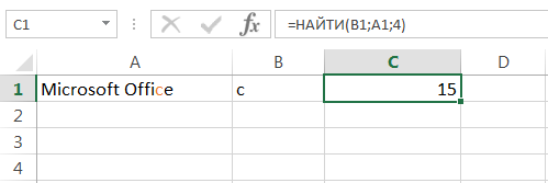
НАЙТИ

Текстовая функция НАЙТИ находит вхождение одной строки в другую и возвращает положение первого символа искомой фразы относительно начала текста.

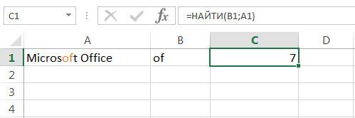
Данная функция чувствительна к регистру…

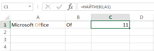
… и может начинать просмотр текста с указанной позиции. На рисунке ниже формула начинает просмотр с четвертого символа, т.е. c буквы «r«. Но даже в этом случае положение символа считается относительно начала просматриваемого текста.

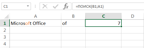
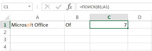
ПОИСК

Текстовая функция ПОИСК очень похожа на функцию НАЙТИ, основное их различие заключается в том, что ПОИСК не чувствительна к регистру.

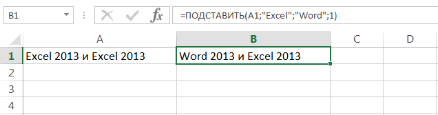
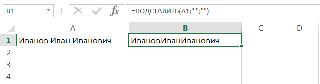
ПОДСТАВИТЬ

Заменяет определенный текст или символ на требуемое значение. В Excel текстовую функцию ПОДСТАВИТЬ применяют, когда заранее известно какой текст необходимо заменить, а не его местоположение.

Приведенная ниже формула заменяет все вхождения слова «Excel» на «Word»:

Заменяет только первое вхождение слова «Excel»:

Удаляет все пробелы из текстовой строки:

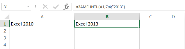
ЗАМЕНИТЬ

Заменяет символы, расположенные в заранее известном месте строки, на требуемое значение. В Excel текстовую функцию ЗАМЕНИТЬ применяют, когда известно где располагается текст, при этом сам он не важен.

Формула в примере ниже заменяет 4 символа, расположенные, начиная с седьмой позиции, на значение «2013». Применительно к нашему примеру, формула заменит «2010» на «2013».

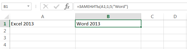
Заменяет первые пять символов текстовой строки, т.е. слово «Excel», на «Word».

Вот и все! Мы познакомились с 15-ю текстовыми функциями Microsoft Excel и посмотрели их действие на простых примерах. Надеюсь, что данный урок пришелся Вам как раз кстати, и Вы получили от него хотя бы малость полезной информации. Всего доброго и успехов в изучении Excel!

При использовании Excel часто необходимо работать не только с числами, но и с текстом. В этой статье мы разберем 12 основных функций Excel для обработки текста.

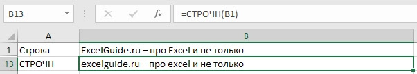
Для примера возьмем строку «ExcelGuide.ru – про Excel и не только» и ее будем использовать в наших функциях ниже.

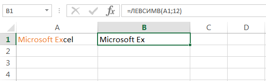
ЛЕВСИМВ

Функция ЛЕВСИМВ возвращает указанное количество знаков с начала строки. В качестве аргументов на первом месте указываем ту строку, из которой хотим извлечь текст, а вторым аргументом количество символов, которое хотим получить.
Давайте из нашей строки получим текст «ExcelGuide.ru»:

=ЛЕВСИМВ(B1;13)

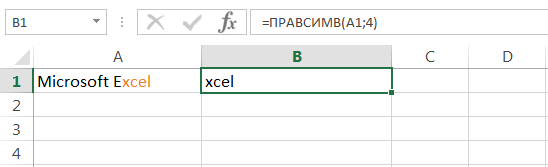
ПРАВСИМВ

Функция ПРАВСИМВ аналогична ЛЕВСИМВ, только возвращает указанное количество символов не с начала, а с конца строки. Первым аргументом указываем строку, откуда будем получать часть текста, а вторым аргументом – количество символов.
Из нашей строки извлечем текст «про Excel и не только»:

=ПРАВСИМВ(B1;21)

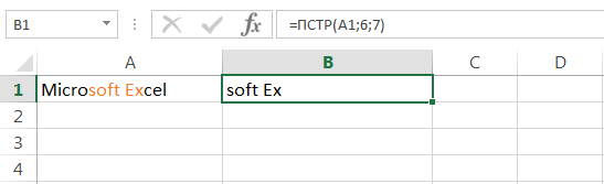
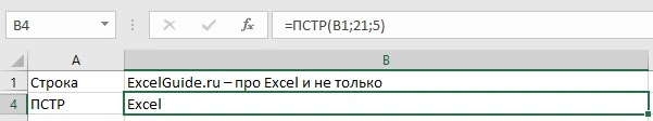
ПСТР

Функция ПСТР позволяет получить указанное количество символов начиная с определенной позиции. У этой функции 3 аргумента: Текст, из которого нам нужно получить часть; стартовая позиция, с которой нужно извлечь символы; количество символов, которое хотим получить.
В нашей строке есть слово Excel, давайте его получим:

=ПСТР(B1;21;5)

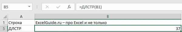
ДЛСТР

Функция ДЛСТР возвращает количество символов в строке.

=ДЛСТР(B1)

ПОИСК

Функция ПОИСК предназначена для нахождения первого вхождения указанного текста в исходную строку. Аргументы функции: сначала указываем тот текст, который хотим найти; далее строку, в которой ищем текст.
Давайте в нашем примере найдем текст «про Excel»:

=ПОИСК(«про Excel»;B1)

СЦЕПИТЬ

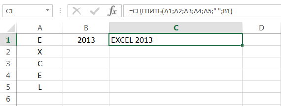
Функция СЦЕПИТЬ позволяет последовательно объединить несколько текстовых элементов в одну строку.
В качестве аргументов необходимо перечислить те текстовые элементы, которые вы хотите соединить.
 В качестве примера объединим наш пример и строку «. Пожалуй лучший сайт про Excel )))»:

=СЦЕПИТЬ(B1;». Пожалуй лучший сайт про Excel )))»)

СОВПАД

Функция СОВПАД проверяет идентичность двух строк и возвращает Истина, если строки совпадают и ЛОЖЬ, если строки не совпадают.
Сравним нашу строку с текстом «ExcelGuide.ru»:

=СОВПАД(B1;»ExcelGuide.ru»)

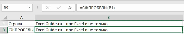
СЖПРОБЕЛЫ

Функция СЖПРОБЕЛЫ удаляет лишние дублирующие пробелы. В качестве аргумента указываем строку, у которой надо удалить лишние пробелы.

=СЖПРОБЕЛЫ(B1)

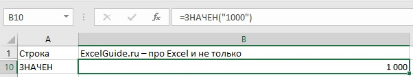
ЗНАЧЕН

Функция ЗНАЧЕН преобразует текст в число. Часто случается при экспорте из разных информационных систем мы получаем числовые значения в текстовом формате, в таких случаях нам и пригодится этот функционал.
В качестве примера преобразуем текст «1000» в число 1 000:

=ЗНАЧЕН(«1000»)

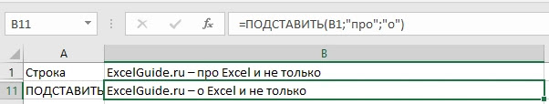
ПОДСТАВИТЬ

Функция ПОДСТАВИТЬ заменяет новым текстом старый текст в исходной текстовой строке. Аргументов у функции три: сначала указываем ту строку, в которой будем менять текст; далее указываем старый текст; а затем тот, которым мы хотим заменить.
В качестве примера в нашей строке заменим «про» на «о»:

=ПОДСТАВИТЬ(B1;»про»;»о»)

ПРОПИСН

Функция ПРОПИСН преобразует все буквы в прописные. У функции только один аргумент – та строка, которую надо преобразовать.

=ПРОПИСН(B1)

СТРОЧН

Функция СТРОЧН преобразует все буквы в строчные. У функции один аргумент – тот текст, который мы хотим модифицировать.

=СТРОЧН(B1)

Кстати, если вы хотите более подробно изучить Excel, научиться строить быстро сложные отчеты и графики, то рекомендую вам курс «Excel + Google Таблицы с нуля до PRO» от Skillbox.

Спасибо за внимание. Мы разобрали 12 основных текстовых функций в Excel, которые вам могут пригодиться в ежедневной работе.