Word formulas for excel

Ok, Ok, Chandoo.org is clearly a Microsoft Excel centric Blog.

But a week ago Pradeep asked the question in a post, “How do I add up a Table of Numbers in Word?”

There are 3 easy answers, which will all be addressed in this post:

1. Transfer the Data to/from Excel
2. Embed a Table in Word from Excel
3. Do the Maths in Word

Transfer Data To/From Excel

The easiest and sometimes quickest way to do maths on a table of numbers is to:

• Copy the Table from Word and paste the Table into an Excel Workbook
• Perform the Maths in Excel
• Copy and paste the results back

Here is a typical Table within Word

Select the Table in Word and press either Ctrl+C or use the Copy icon.

Open Excel or switch to Excel using Alt+Tab

Select a cell and press Paste Ctrl+V or use the Paste  Icon

Excel shows the Table as above.

Next add formulas to perform the calculations you need

In this case in C9: =SUM(C4:C8)

Copy the formula in C9 across to D9

In E4: =D4/C4

Copy the formula in E4 down to E9

Format the new results as appropriate

Next select either the full table or a section, ie: The Numbers and Copy using either Ctrl+C or use the Copy icon.

Switch to Word using Alt+Tab

Select the same area in the Word Table as what you copied in Excel

and press Paste Ctrl+V or use the Paste  Icon

When to use this technique

This technique is useful for doing one of reports where the data is provided to you as is.

It is also good when you need to perform complex formulas.

However when you control the data source there is an easier way and this is discussed next.

Embed the Table in Word from Excel

In cases where you manage the data source, you can link the table in Word directly to the data source in Excel.

By doing this the Word Table is updated as soon as changes are made in the Excel Table.

In Excel find your source data:

Select the range you want to embed into the word Document

Copy this range using either Ctrl+C or use the Copy icon.

Open Word or Switch to Word using Alt+Tab

Locate and click in the area in the Word Document where you want to place the report

Goto the Home Tab and press Paste Ctrl+V or use the Paste  Icon

Select the Paste and Keep Source Formatting option

Note 1: As you move across the 6 paste options word will show you what the Pasted range will look like using each format

Note 2: Notice in the example above the pasted range also includes the grey grid lines. If you don’t want these you need to disable them in Excel before you copy the range

Now that we have our Word Document with the new Range pasted in, you notice that there is a mistake in the data

Return to Excel by Using Alt+Tab

Change the Date to the 18 Aug 2018 and change the Revenue on Tuesday to 3000

Return to Excel by Using Alt+Tab

Notice that the Date, Tuesday Revenue and Unit Revenue have all changed to reflect the changes in the excel Document.

You can reformat the Table in Word and only the numbers and text will change in response to changes in the Excel Document

The Excel and Word Files must be open for the link to be updated dynamically.

If the Excel file is closed the Word file will not update.

When to use this technique

This is a great technique when you have a large data source with mutiple tables used in Word, Like a Monthly Report.

But there is an alternative…

Perform the Maths in Word

Microsoft Word has limited arithmetic abilities built in.

These abilities only apply to data stored in Tables, not to data stored in tabular format within normal text

Open a word file and enter a Table of Data like below

This is the same table we have seen before.

It requires a Total Line as well as Unit Revenue calculations

Click into the Sales Quantity Weekly Totals cell.

Now goto the Layout Tab and select the Formula icon.

In the Formula: dialog Word will have inserted a Formula =SUM(ABOVE)

This is what we want to do, so leave it

Select an appropriate Number format from the Number format drop down. These number formats are in the same style as Excel Custom Number Formats.

Click OK

Word puts the total 750 in this case in the Total cell

Change a Number above and watch as the Total changes

Repeat the previous step in the revenue Weekly Total cell

The Unit Revenue will be the Revenue for each day divided by the Sales Quantity that day.

That is, for Monday, we want to divide the Sales Revenue of $2,000 by the Sales Quantity 100 to return a Unit Revenue of 200

Luckily Word has the facility to treat Cells in a Table in a similar fashion to Excel !

We can use either R1C1 or A1 formula formats.

In R1C1 each column and row is simply numbered as shown below

In A1 each column is Labelled alphabetically as in the default view in Excel and row is numbered as shown below

And Word is actually more advanced than Excel as you can use either format at the same time without having to change the format in settings.

In our example we want to divide the Cell in Row 2 Column 3 (R2C3) by the value in Row 2 Column 2 (R2C2)

Click in the Cell under the Unit Revenue column header in Row 2

Goto the Layout Tab and select the Formula icon

By default Word will display a =SUM(LEFT) formula

Overwrite this with your own formula =R2C3/R2C2

Select an appropriate Number format and press OK

You can use the A1 formula style by simply using it

Click in the Cell under the Unit Revenue column header in Row 2

Goto the Layout Tab and select the Formula icon

By default Word will display a =SUM(LEFT) formula

Overwrite this with your own formula =C2/B2

Select an appropriate Number format and press OK

Repeat this for the other cells in the Unit Revenue column.

Voila !

You now have a Table in Word, the Total and Unit Rates are Formulas.

But wait there is a mistake, The Revenue on Tuesday should be $5,000

Select the cell and change the value to 5,000

Depending on which version of Word you have the Table will either Update Automatically or you can force it to recalculate

If you Change the Value and the Table updates itself, Enjoy it

If your Table hasn’t updated itself you have a few options

Select the cells by Left Click and Drag ie: From 5,000 Down to the base of the table and across to the Right

Now Right click the selection and select Update or press F9

You can also click on an individual cell within the Table and Right Click and Update

Or you can press Ctrl+A outside the Table and Right Click and Update or Press F9

What Other Functions are Available?

We saw in the example above that we can use basic operands of +, –, * and /

We used the function Sum()

But there are about a dozen other functions available to us to construct formula to process our data

To see and use these Goto the Layout Tab and select the Paste function dropdown on the Formula Dialog.

Scroll down to see other functions

You can build up a function as you do in Excel using parenthesis and these functions.

In the example above we used the special Above range to specify that we wanted to Sum the values Above the active cell.

You can also use the LEFT, RIGHT, ABOVE, BELOW positional arguments

If you have defined Bookmarks within the Word document you can also use these to return values

=ROUND(NPV,0)

Where NPV is a Bookmark to the value of the NPV elsewhere in your Document.

Further Help

Word has a good discussion on the techniques available in the online help

Microsoft Word – Formula in a cell help

Final Comments

How have you performed maths on data in Word?

Let us know in the comments below:

Excel formulas let you automate your spreadsheets. But how do you use it in a Word document? Here are two ways to do it!

While you can always integrate Excel data into a Word document, it’s often unnecessary when all you need is a small table. It’s quite simple to create a table and use Excel formulas in a Word document. However, there is only a limited number of formulas that can be used.

For instance, if you’re trying to insert sales data in a table, you could add a column for sales, another one for total cost, and a third one for calculating profit using a formula. You can also calculate an average or a maximum for each of these columns.

Method 1: Paste Spreadsheet Data Into Word

If you already have data populated into a spreadsheet, you could just copy it into your Microsoft Word document.

1. Copy the cells containing the data and open a Word document.
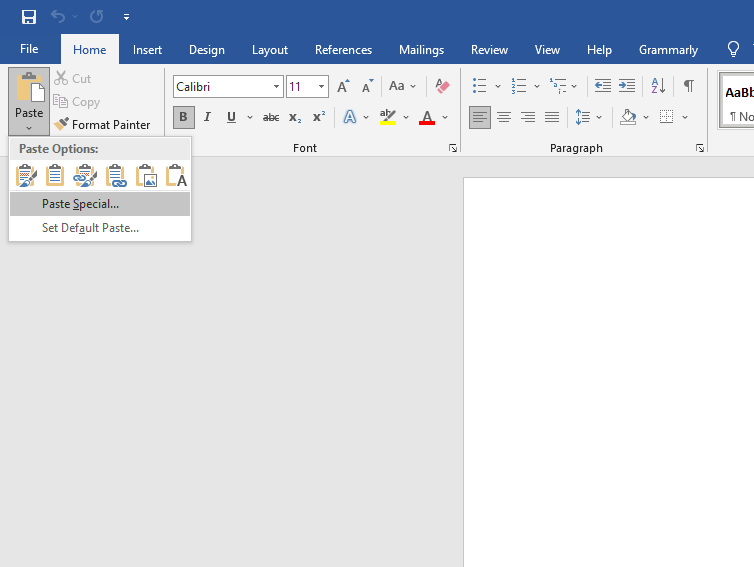
2. From the top ribbon, click on the arrow under the Paste button, and click on Paste Special.
   
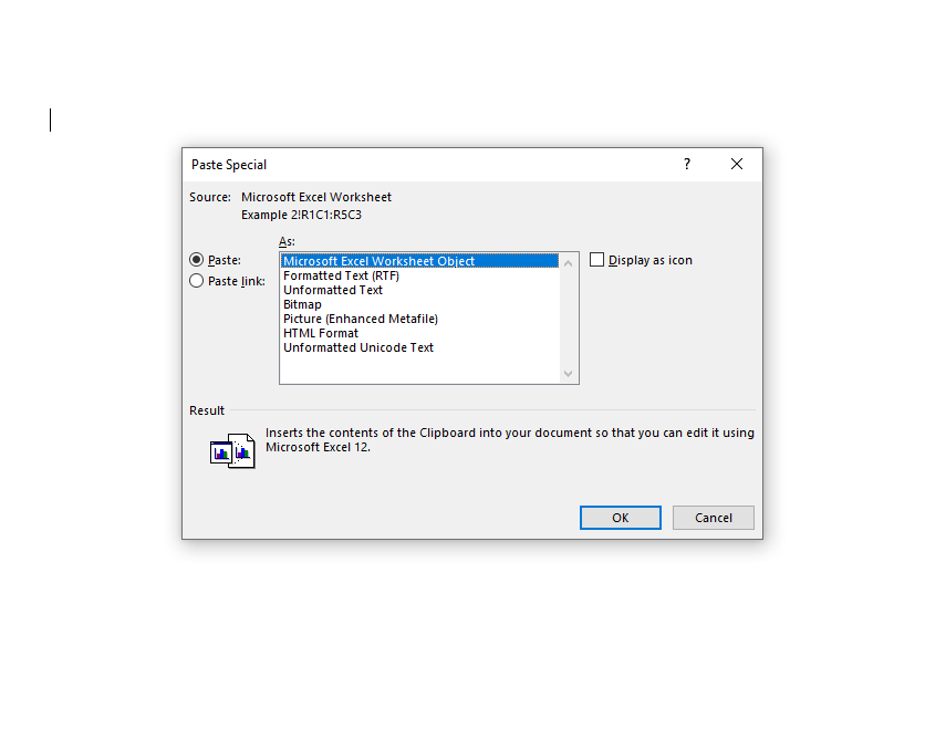
3. You’ll see a new window pop-up where you’ll need to select what you want to paste the copied content as. Select Microsoft Excel Worksheet Object and select OK.
   
4. Your data should now appear in the Word document, and the cells should contain the formulas as well.

If you want to make any edits, you can double-click on the pasted content, and your Word document will transform into an Excel document, and you’ll be able to do everything you would on a normal spreadsheet.

Method 2: Add Formulas in a Table Cell in Word

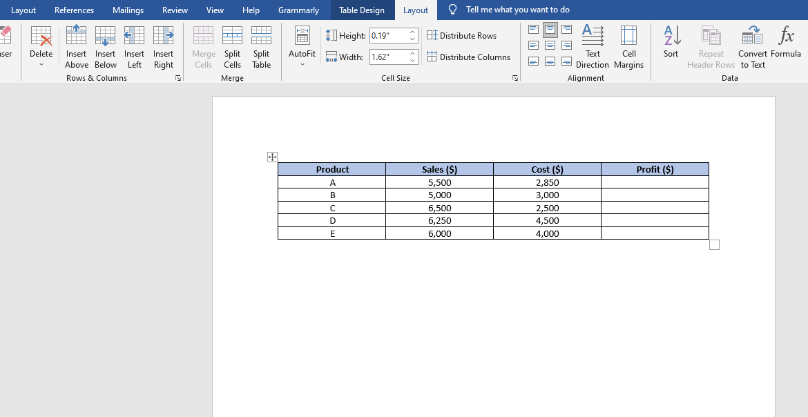
1. Quickly insert a table in your Word document and populate the table with data.
2. Navigate to the cell where you want to make your computations using a formula. Once you’ve selected the cell, switch to the Layout tab from the ribbon at the top and select Formula from the Data group.
   

   Notice that there are two tabs called Layout. You need to select the one that appears under Table Tools in the ribbon.

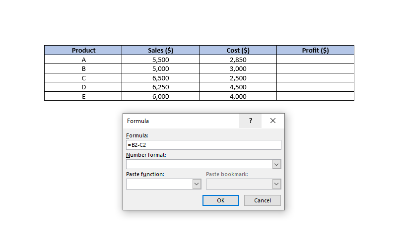
3. When you click on Formula, you’ll see a small window pop up.
4. The first field in the box is where you enter the formula you want to use. In addition to formulas, you can also perform basic arithmetic operations here. For instance, say you want to compute the profit, you could just use the formula:

    =B2-C2 

   Here, B2 represents the second cell in the second column, and C2 represents the second cell in the third column.

   
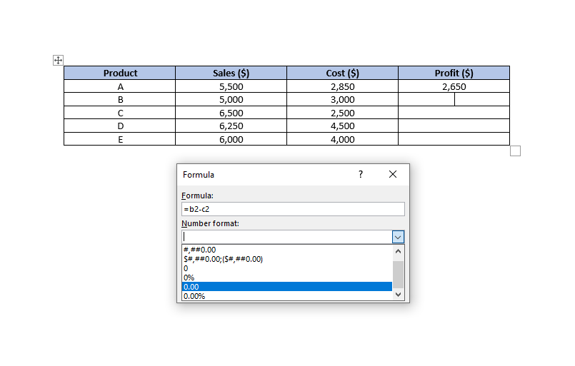
5. The second field allows you to set the Number Format. For instance, if you wanted to calculate profit down to two decimal places, you could select a number format accordingly.
   
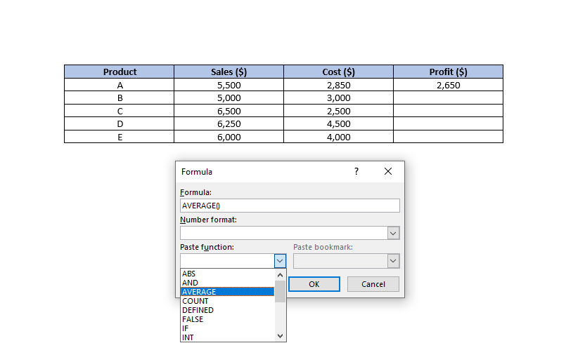
6. The Paste Function field lists the formulas you can use in Word. If you can’t remember the name of a function, you could select one from the dropdown list, and it will automatically be added to the Formula field.
   
7. When you’ve entered the function, click OK, and you’ll see the computed figure in the cell.

Positional Arguments

Positional arguments (ABOVE, BELOW, LEFT, RIGHT) can often make things simpler, especially if your table is relatively large. For instance, if you have 20 or more columns in your table, you could use the formula =SUM(ABOVE) instead of referencing each cell inside the parenthesis.

You can use positional arguments with the following functions:

• SUM
• AVERAGE
• MIN
• MAX
• COUNT
• PRODUCT

For instance, we could calculate the average sales for the above example using the formula:

 =AVERAGE(ABOVE) 

If your cell is at the center of the column, you can use a combination of positional arguments. For instance, you could sum up the values above and below a specific cell using the following formula:

 =SUM(ABOVE,BELOW) 

If you want to sum up the values from both the row and the column in a corner cell, you could use the following formula:

 =SUM(LEFT,ABOVE) 

Even though Microsoft Word offers only a few functions, they are quite robust in functionality and will easily help you create most tables without running into lack-of-functionality issues.

Updating Data and Results

Unlike Excel, Microsoft Word doesn’t update formula results in real-time. However, it does update the results once you close and re-open the document. If you want to keep things simple, just update the data, close, and re-open the document.

However, if you’d like to update the formula results as you continue to work on the document, you’ll need to select the results (not just the cell), right-click on them, and select Update Field.

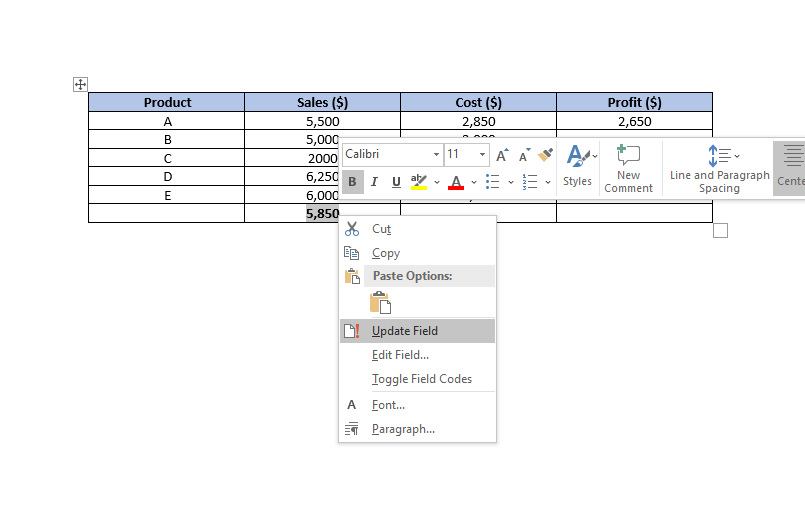
When you click Update Field, the formula’s result should update instantly.

Cell References

There are several ways to reference a cell in a Word document.

1. Bookmark Names

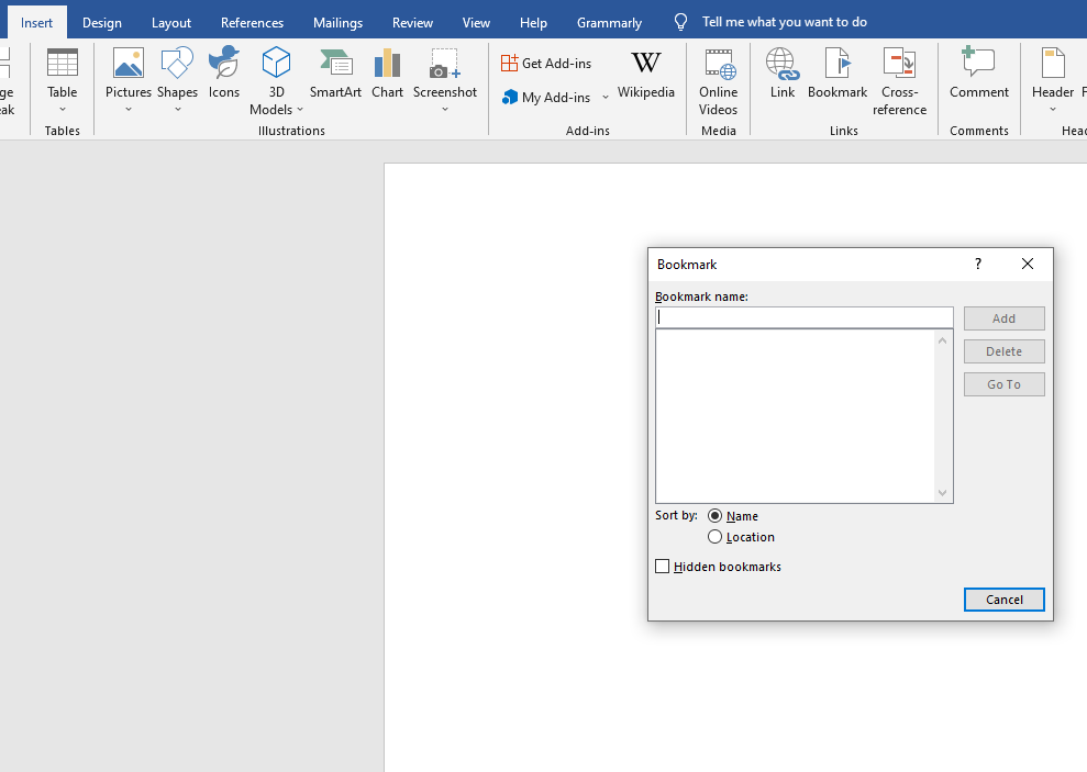
Let’s say you give your average sales value a bookmark name average_sales. If you don’t know how to give a cell a bookmark name, select the cell and navigate to Insert > Bookmark from the ribbon at the top.

Assume that the average sales value is a decimal value, and you’d like to convert it to an integer. You could reference the average sales value as ROUND(average_sales,0), and this will round the value down to its nearest integer.

2. RnCn References

The RnCn referencing convention allows you to reference a row, column, or a specific cell in a table. The Rn refers to the nth row, while the Cn refers to the nth column. If you wanted to refer to the fifth column and second row, for instance, you’d use R2C5.

You can even select a range of cells using the RnCn reference, much like you would in Excel. For instance, selecting R1C1:R1C6 selects the first six cells of the first row. For selecting the entire row in which you’re using the formula, just use R (or C for a column).

3. A1 References

This is the convention that Excel uses, and we’re all familiar with. The letter represents the columns, while the numbers represent the rows. For instance, A3 refers to the third cell in the first column.

Word Tables Made Easy

Hopefully, the next time you’ll need to use data on a Microsoft Word document, you’ll be able to do things much faster without having to first create a spreadsheet and then import it into your Word document.

When you are cleaning up data in Excel, the Text-to-Columns and Flash Fill features are awesome, but sometimes you need to use formulas to manipulate text. In this article I’ll demonstrate examples of the text formulas I commonly use, including LEN, TRIM, UPPER, LOWER, PROPER, CONCATENATE, INDIRECT, CHAR, FIND, SEARCH, SUBSTITUTE, LEFT, RIGHT, MID and REPLACE (and some others).

The examples start very simple and then get progressively more advanced as you scroll through the page, building upon earlier examples.

Download the Example File (TextFormulas.xlsx)

Do you have a text manipulation challenge that you need a formula to solve? Feel free to ask your question by commenting below.

1. Get the LENgth of a text string

=LEN("onetwothree")
Result: 11

This comes in handy when you need to write a title for a web page or complete a form with a limited number of characters. Just open a blank spreadsheet and type your title in cell A1. In B1, enter =LEN(A1).

2. Change case to UPPER, lower, or Proper

=UPPER("this text")   Result: THIS TEXT
=LOWER("THIS TEXT")   Result: this text
=PROPER("this text")   Result: This Text

3. Concatenate a text string

You can use CONCATENATE, the & operator, or the newer CONCAT and TEXTJOIN functions to concatenate strings. The following formulas combine a first name in cell A1 and a last name in cell B1 with a space in the middle. The result is «John Smith» for all four formulas.

A1="John"
B1="Smith"

=A1 & " " & B1
=CONCATENATE(A1," ",B1)
=CONCAT(A1:B1)
=TEXTJOIN(" ",TRUE,A1:B1)

Result: "John Smith"

NOTE The spaces before and after the & operator are not required — I’ve included the spaces only to help make the formula more readable.

The CONCAT and TEXTJOIN functions are new functions that requires an Office 365 subscription (they work in Excel Online). The CONCAT function is like CONCATENATE except that it lets you use a range of cells as an argument. The TEXTJOIN function lets you specify a delimiter and ignore blank values.

4. Use INDIRECT to create a reference from a text string

The INDIRECT function allows you to create a reference from a text string. The example below shows a reference to cell A5 in worksheet ‘Sheet 2’. The single quotes around the worksheet name are only necessary if the worksheet name includes a space.

=INDIRECT("'Sheet 2'!A5")

Use INDIRECT if you want the worksheet name to be a text string chosen by the user. For example, you may want to do this if you have many identical worksheets and you want to create a summary table that uses the names of those worksheets as references in your lookup formulas.

The following example creates a reference to cell X5 in a worksheet that is named in cell A1.

A1="Sheet 2"
A2=INDIRECT("'" & A1 & "'!X5")

The INDIRECT function can be very useful in array formulas. For example, to create an array of numbers 1 through N, where N is a number contained in cell A1, you can use:

=ROW(INDIRECT("1:" & A1))

5. Use CHAR to return special characters

The CHAR function lets you return a character for a given numeric code. The UNICHAR function returns a character for a decimal Unicode value. Although most of the numeric codes for the CHAR function correspond to the ASCII codes, some may not be the same (such as codes 128-160).

The functions CODE and UNICODE are the opposites of CHAR and UNICHAR, returning the numeric value for the first character in a text string.

Use CHAR(34) to return the double quote » character

When you concatenate text and need to include double quotes in the displayed text, you can use the CHAR(34) or UNICHAR(34) function. Both the ASCII and Unicode value for double quotes is 34.

=CHAR(34) & "Hi World" & CHAR(34)
Result: "Hi World" (quotes included)

Use CHAR(10) to include a line break in a string

When using a formula to return a string, use CHAR(10) or UNICHAR(10) for a line break. See Custom Number Formats to learn how to add a line break within a custom number format (for chart labels and stuff like that).

="abc" & CHAR(10) & "def"
Result:
abc
def

! To display wrapped text with line breaks, the cell must also have the Word Wrap property toggled on.

TIP To quickly generate a list of characters based on their numeric code, enter =CHAR(ROW()) or =UNICHAR(ROW()) into cell A1 of a blank worksheet and copy the formula down.

See my article «Using UNICODE Characters in Excel» for more information.

6. SUBSTITUTE text within a string

The SUBSTITUTE function is very powerful. It can be used to replace ether ALL occurrences or just the Nth occurrence of a string with another character or text string. In the example below, we’re replacing the # character with a space.

text = "one#two#three"
=SUBSTITUTE(text,"#"," ")   Result: "one two three"
=SUBSTITUTE(text,"#"," ",2)   Result: "one#two three"

7. Use TRIM to get rid of extra spaces

The TRIM function removes all regular spaces (ASCII character 32) except for a single space between words.

=TRIM("   Hi  World  ")
Result: "Hi World"  (quotes not included)

TRIM does not remove tabs, line breaks, or other nonprinting characters from the text. To remove the non-printing ASCII characters 0-31 (including the tab character), you can use the CLEAN function.

text="Hi		World" (contains two tabs)
=CLEAN(text)
Result: "HiWorld"

The problem with the CLEAN function is that it completely removes the characters, so words separated by tabs or newline characters will be combined, so you may end up with «HiWorld» when you would prefer «Hi World».

To change special characters to regular spaces, you can use the SUBSTITUTE function and then wrap the function with TRIM to remove extra spaces like this:

text="Hi		World" (contains two tabs)
=TRIM( SUBSTITUTE(text,CHAR(9)," ") )
Result: "Hi World"

NOTE Here is a short list of CHAR codes for commonly replaced characters: Tab (9), Newline (10), Carriage Return (13), Space (32), Non-Breaking Space (160), Special Quote Symbols: ‘(145), ’(146), “(147), ”(148)

8. Use FIND and SEARCH to get the position of text in a string

The FIND function for case-sensitive searching and the SEARCH function for case-insensitive searching will return the starting character position of a text string within another string.

=FIND("a","ooAooaoo",1)   Result: 6
=SEARCH("a","ooAooaoo",1)   Result: 3

The 3rd argument of the FIND and SEARCH functions is the starting character position to begin the search, with the default being 1 (the first character). You can use a nested FIND or nested SEARCH to find the position of the 2nd occurrence of a text string like this:

text="ooAooAoo"
=FIND("A",text,FIND("A",text,1)+1)

Evaluation Steps
Step 1: FIND("A","ooAooAoo",3+1)
Step 2: FIND("A","ooAooAoo",4)
Step 3: 6

You can do some really tricky things with SUBSTITUTE when combined with FIND or SEARCH. The following function allows you to find the location of the Nth occurrence of a string within another text string. In this example, we want to know the position of the 3rd space in the name.

text="Tim A. J. Crane"
=FIND("#",SUBSTITUTE(text," ","#",3),1)

Evaluation Steps
Step 1: =FIND("#","Tim A. J.#Crane",1)
Step 2: =10

9a. Use MID, LEFT and RIGHT to extract text from a string

The MID function is like the substr() function in other coding languages. It extracts a string from within another string by specifying the starting character position and the number of characters to extract. The REPLACE function is similar except that it returns the original text string with the text replaced. The LEFT and RIGHT functions are like shorthand versions of MID for extracting text from the left or right end of a string.

SYNTAX: =MID(text,start_num,num_chars)
SYNTAX: =REPLACE(text,start_num,num_chars,replace_text)
SYNTAX: =LEFT(text,num_chars)
SYNTAX: =RIGHT(text,num_chars)

Below is an example showing how these functions work.

text = "one#two#three"
=MID(text,5,3)   Result: "two"
=REPLACE(text,5,3,"BLAHBLAH")   Result: "one#BLAHBLAH#three"
=LEFT(text,5)   Result: "one#t"
=RIGHT(text,7)   Result: "o#three"

I haven’t had much use for the REPLACE function, because I typically use SUBSTITUTE instead of REPLACE.

The MID, LEFT, and RIGHT functions become much more powerful when you use the FIND or SEARCH functions within them. Some of the following tips show examples of that.

9b. Use the New TEXTAFTER and TEXTBEFORE functions!

New text functions are coming soon to the latest version of Excel. Like their names suggest, TEXTAFTER and TEXTBEFORE let you extract text after or before the nth instance of a delimiter. Some of the complex stuff done with the MID function can be done more easily with these new functions.

SYNTAX: =TEXTAFTER(text,delimiter,[n],[ignore_case])
SYNTAX: =TEXTBEFORE(text,delimiter,[n],[ignore_case])

Using the text from the MID function above, here are a couple examples:

text = "one#two#three"
=TEXTAFTER(text,"#",2)   Result: "three"
=TEXTBEFORE(text,"#",2)   Result: "one#two"

If you enter a negative value for n, it will count the instance from the end of the string. This will come in handy when you need to extract the last part of the string but you don’t know how many delimiters there will be.

10. Count the number of spaces in a text string

You can use this technique to count other characters besides spaces. For example, just substitute » » with «,» or «;» to count the number of commas or semi-colons.

text = "Todd Allen Smith"
=LEN(text)-LEN(SUBSTITUTE(text," ",""))

Evaluation Steps
Step 1: LEN("Todd Allen Smith")-LEN("ToddAllenSmith")
Step 2: 16-14
Step 3: 2

The SUBSTITUTE function in this example returns a new text string with the spaces removed (replacing all » » with «»). We are subtracting the length of that modified text string from the original length to calculate the number of spaces in the original text.

11. Count occurrences of a string within text

If you want to count the number of occurrences of a string within text (instead of just a single character), then you can use a slightly modified version of the above formula. In this case, we’ll just divide the result by the length of string.

text = "A##B##C"
string = "##"
=(LEN(text)-LEN(SUBSTITUTE(text,string,""))) / LEN(string)
Result: 2

12. Split text into columns using formulas

The Text-to-Columns Wizard and Flash Fill (Ctrl+e) features in Excel are fast and simple to use, but there may be times when you want to use formulas instead (to make a more dynamic or automated worksheet). Splitting up text using formulas typically involves a combination of LEFT, RIGHT, MID, LEN, and FIND (or SEARCH). We’ll start with a couple simple formulas.

Extract the First Name

To extract the first word (or name) from a text string, you can use the following formula, where text is either a cell reference or a string surrounded by double quotes like «this».

text = "Tom Sawyer"
=LEFT(text,FIND(" ",text)-1)

Evaluation Steps
Step 1: =LEFT("Tom Sawyer",4-1)
Step 2: =LEFT("Tom Sawyer",3)
Step 3: ="Tom"

In the above formula, FIND(» «,text) returns the numeric position of the first space » » within the text. We subtract one from that value so the space is not included in the result.

The new TEXTBEFORE function is easier (the default for the instance number is 1):

=TEXTBEFORE("Tom Sawyer"," ")  Result: "Tom"

Extract the Text After the First Space

To return the rest of the string after the first space, we use the RIGHT function, which extracts a specified number of characters from the end of the string. We calculate the number of characters to extract by subtracting the position of space from the total length of the string:

text = "Jay Allen Reems"
=RIGHT(text,LEN(text)-FIND(" ",text))

Evaluation Steps
Step 1: =RIGHT("Jay Allen Reems",LEN("Jay Allen Reems")-4)
Step 2: =RIGHT("Jay Allen Reems",15-4)
Step 3: =RIGHT("Jay Allen Reems",11)
Step 4: ="Allen Reems"

The new TEXTAFTER function is easier (the default for the instance number is 1):

=TEXTAFTER("Jay Allen Reems"," ")  Result: "Allen Reems"

We could repeat these formulas in other columns to extract Allen and then Reems.

The article «Split text into different columns with functions» on support.office.com provides various examples of formulas for separating names into different parts based on different ways that a name may be written.

The SPLIT function in Google Sheets

I hope that Excel eventually includes a SPLIT function like the one available in Google Sheets. For example, to split a name like «Allen James Reems» into separate cells only requires the following simple formula:

=SPLIT(text," ")

New TEXTSPLIT function in Excel!

The new TEXTSPLIT function will soon be available in the latest version of Excel. It isn’t exactly the same as the Google Sheets SPLIT function. It’s better in my opinion because it can split text into a row, column, or two-dimensional dynamic array.

SYNTAX: =TEXTSPLIT(text,[column_delimiter],[row_delimiter],[ignore_empty],[pad_width])

You can read more about TEXTSPLIT at MyOnlineTrainingHub.com.

13. Get the last word in a string

For this example, we’ll use the name «Allen Jay Reems» to show how to get the last word in a string, where a space character is the delimiter.

This will soon be very easy with the TEXTAFTER function (see 9b above):

=TEXTAFTER("Allen Jay Reems"," ",-1)   Result: "Reems"

The following example shows how to do this if TEXTAFTER is not available, and also shows how I sometimes build a more complicated formula using intermediate steps.

delimiter = " "
last_name
   =RIGHT(text,LEN(text)-position_of_last_delimiter)
position_of_last_delimiter
   =FIND("^", SUBSTITUTE(text,delimiter,"^",number_of_delimiters))
number_of_delimiters
   =LEN(text)-LEN(SUBSTITUTE(text,delimiter,""))

The final formula looks like this with A1=»Allen Jay Reems» and will return the last name «Reems»:

=RIGHT(A1,LEN(A1)-FIND("^", SUBSTITUTE(A1," ","^",LEN(A1)-LEN( SUBSTITUTE(A1," ","") ))))

If you have a string delimited by commas like «one, two, three, four» you can extract the last element by replacing » » with «,» in the above formula and wrapping the entire thing with TRIM to remove the leading space.

If your string might not contain any spaces, then you can wrap the entire formula with IFERROR to return an empty string or the original text.

If your string contains the «^» character, you’ll need to choose a different temporary delimiter to use in the formula such as «~» or another uncommonly used character.

14. Get the Nth word in a string

This is another task that will be much simpler with the new TEXTBEFORE function. Using the example below:

=TEXTBEFORE(TEXTBEFORE("One#Two#Three",2),-1)
Evaluation Steps
1: =TEXTBEFORE("One#Two",-1)
2: ="Two"

Without the new functions, this formula is really crazy, but still useful. I learned it from a post on mrexcel.com. Basically what is going on is that you replace the delimiter text with a bunch of blank spaces so that you create a new text string that can be divided into chunks, where each chunk contains a different word. There will be a lot of space surrounding each word, so you use TRIM to remove it.

text = "One#Two#Three" (the original text)
delimiter = "#" (the delimiter text)
word_num = 2 (the word to extract)

=TRIM(MID(SUBSTITUTE(text,delimeter,REPT(" ",LEN(text))),(word_num-1)*LEN(text)+1,LEN(text)))

Evaluation Steps
1: =TRIM(MID(SUBSTITUTE(text,"#",REPT(" ",13)),(2-1)*13+1,13))
2: =TRIM(MID(SUBSTITUTE(text,"#","             "),14,13))
3: =TRIM(MID("One             Two             Three",14,13))
4: =TRIM("  Two        ")
5: ="Two"

In Google Sheets, this is a piece of cake. The SPLIT function returns an array, so you can return the 3rd word in a string using:

=INDEX(SPLIT(text,delimiter),3)

15. Convert a text string to an array of words

Want to convert «One#Two#Three» into an array like {«One»;»Two»;»Three»} that can be used within other formulas? That is what the SPLIT function in Google Sheets does, but to do this in Excel is still possible — it’s just complicated. First, start with the formula in the previous section and replace word_num with the following:

=ROW(INDIRECT("1:"&((LEN(text)-LEN(SUBSTITUTE(text,delimiter,"")))/LEN(delimiter)+1)))

To display the results within an array of cells, remember to use Ctrl+Shift+Enter. Use TRANSPOSE if you want to display the results of this formula in a row instead of a column.

To create the array as an inline text string, you can use the following formula:

text = "One#Two#Three" (the original text)
str = "#" (the delimiter text)
="{"&CHAR(34)&SUBSTITUTE(text,str,CHAR(34)&";"&CHAR(34))&CHAR(34)&"}"

Resulting text string: {"One";"Two";"Three"}

16. Convert a text string to an array of characters

If you want to split a text string into an array of individual characters, such as converting «abcd» to {«a»;»b»;»c»;»d»}, the formula is fairly simple. This formula is entered as an Array Formula (Ctrl+Shift+Enter).

=MID(text_string,ROW( INDIRECT("1:"&LEN(text_string)) ),1)

To convert each of the characters in a string to their numeric codes, wrap the above function with CODE or UNICODE. The formula would be entered as a multi-cell array to display each of the numeric values in a different cell.

The following formula in Google Sheets will convert a text string to a comma-delimited list of numeric code values.

text="Hello"
=ARRAYFORMULA( TEXTJOIN(",",TRUE, CODE(MID(text,ROW( INDIRECT("1:"&LEN(text)) ),1))) )
Resulting text string: "72,101,108,108,111"

17. Use EXACT for case-sensitive text comparisons

If you ever need to determine if the text in a cell is UPPERCASE, lowercase, or Proper Case, you can use the EXACT formula to compare the original text to the converted text.

The following formulas return TRUE if the text in cell A1 is uppercase, lowercase or proper case, respectively:

=EXACT(A1,UPPER(A1))
=EXACT(A1,LOWER(A1))
=EXACT(A1,PROPER(A1))

Note: The SUMIF and COUNTIF article provides a lot of different examples of text-based comparisons.

Have a Text Formula Challenge?

If this article hasn’t answered your question, feel free to comment below if you have a problem that you want solved using a text formula. Make sure to provide sufficient detail for your question to be answered. Thank you!

1. 11-01-2016, 01:55 AM

   
   

   #1

   

   
   Registered User
   

   

   ---

   Formulating word formulas for excel
   

   http://www.ozgrid.com/forum/showthread.php?t=201635
   http://www.mrexcel.com/forum/excel-q…help-asap.html

   Hi everyone, I have a problem that I hope someone can help me with. I have a list of postcodes in one sheet and these are assigned an area in the next column.

   e.g. 2000 Sydney
   2060 North Sydney

   I then have another sheet of data with just postcodes (lots of them). I want to use the data from the first sheet to populate the adjacent column in the new sheet.

   i.e. 2000 = some formula to look up the value in the column next to the postcode in the first spreadsheet
   2060 = some formula to look up the value in the column next to the postcode in the first spreadsheet

   The result being:

   2000 Sydney
   2060 North Sydney

   How could i do this?

   Last edited by jen0919; 11-01-2016 at 02:35 AM.

   ---

2. 11-01-2016, 02:18 AM

   
   

   #2

   Re: Formulating word formulas for excel
   

   Maybe like this in B1 of the second sheet?

   =VLOOKUP(A1,Sheet1!$A$1:$B$500,2,0)

   where A1 contains the postcode to be looked up and the array is where your list of codes and regions is to be found.

   Ali

   ---

   Enthusiastic self-taught user of MS Excel who’s always learning!
   Don’t forget to say «thank you» to anyone who has offered you help in your thread. You can reward them by clicking on * Add Reputation below theur user name on the left, if you wish.

   Forum Rules (updated September 2018): please read them here.
   How to use the Power Query code you’ve been given: help here. More about the Power suite here.

   ---

3. 11-01-2016, 02:19 AM

   
   

   #3

   Re: Formulating word formulas for excel
   

   Can you post a sample worksheet?

   I think you can use =VLOOKUP(A2,Sheet1!$A$2:$B$3,2,0)

   

   ---

4. 11-01-2016, 02:20 AM

   
   

   #4

   Re: Formulating word formulas for excel
   

   Read about VLOOKUP or INDEX / MATCH

   sandy

   ---

   I want to see what you are trying to achieve, not how you are trying to do it

   What makes learning so hard is the amount of knowledge you have to unlearn
   Why is my program not doing what I expect?
   Because you set the wrong expectations. Rewire your brain

   

   ---

5. 11-01-2016, 02:23 AM

   
   

   #5

   

   
   Registered User
   

   

   ---

   Re: Formulating word formulas for excel
   

   I’ll try this and let you know. Thank you!

   ---

6. 11-01-2016, 02:23 AM

   
   

   #6

   Re: Formulating word formulas for excel
   

   Your post does not comply with Rule 8 of our Forum RULES. Do not crosspost your question on multiple forums without including links here to the other threads on other forums.

   Cross-posting is when you post the same question in other forums on the web. The last thing you want to do is waste people’s time working on an issue you have already resolved elsewhere. We prefer that you not cross-post at all, but if you do (and it’s unlikely to go unnoticed), you MUST provide a link (copy the url from the address bar in your browser) to the cross-post.
   
   Please add a link in your opening post in this thread: this is not optional. Thanks!

   Read this to understand why we ask you to do this, and then please edit your first post to include links to any and all cross-posts in any other forums (not just this site).

   ---

7. 11-01-2016, 02:23 AM

   
   

   #7

   Re: Formulating word formulas for excel
   

   And please update your thread on Ozgrid for this issue.

   ---

8. 11-01-2016, 02:24 AM

   
   

   #8

   

   
   Registered User
   

   

   ---

   Re: Formulating word formulas for excel
   

   Thank you for the information

   ---

9. 11-01-2016, 02:25 AM

   
   

   #9

   

   
   Registered User
   

   

   ---

   Re: Formulating word formulas for excel
   

   Thanks Ali. Will try it out

   ---

10. 11-01-2016, 02:26 AM

    
    

    #10

    Re: Formulating word formulas for excel
    

    Please add links to your posts on the other forums where you have asked the same question. This is not optional. Thanks!

    Last edited by AliGW; 11-01-2016 at 02:30 AM.

    ---

11. 11-01-2016, 02:32 AM

    
    

    #11

    Re: Formulating word formulas for excel
    

    Thank you for adding the link, but you also need to add a link to the third forum where you have asked the same question.

    ---

12. 11-01-2016, 03:40 AM

    
    

    #12

    Re: Formulating word formulas for excel
    

    Originally Posted by jen0919
    

    I have a list of postcodes in one sheet and these are assigned an area in the next column.

    e.g. 2000 Sydney
    2060 North Sydney

    I then have another sheet of data with just postcodes (lots of them). I want to use the data from the first sheet to populate the adjacent column in the new sheet.

    i.e. 2000 = some formula to look up the value in the column next to the postcode in the first spreadsheet
    2060 = some formula to look up the value in the column next to the postcode in the first spreadsheet

    The result being:

    2000 Sydney
    2060 North Sydney

    Given that there are multiple localities per postcode — and that those localities can even span state boundaries, I suspect you’ll need something rather more elaborate than a single lookup result. Depending on what you’re trying to achieve, you may need to use Dependent Dropdowns and/or Matching with Repeated Data. For examples of these, see-

    Dependent Dropdowns:
    http://windowssecrets.com/forums/sho…474#post861474
    http://www.eileenslounge.com/viewtopic.php?f=27&t=8830

    Matching with Repeated Data:
    http://windowssecrets.com/forums/sho…l=1#post734296
    http://www.techsupportforum.com/foru…ml#post2567119

    Cheers,
    Paul Edstein
    [Fmr MS MVP — Word]

    ---

13. 11-01-2016, 04:21 AM

    
    

    #13

    Re: Formulating word formulas for excel
    

    Thank you for adding the other link.

    ---

14. 11-02-2016, 02:07 AM

    
    

    #14

    

    
    Registered User
    

    

    ---

    Re: Formulating word formulas for excel
    

    Ali, this formula isn’t working. It gives me n/a as a result.

    ---

15. 11-02-2016, 02:08 AM

    
    

    #15

    

    
    Registered User
    

    

    ---

    Re: Formulating word formulas for excel
    

    thank you for the info

    ---

16. 11-02-2016, 02:27 AM

    
    

    #16

    Re: Formulating word formulas for excel
    

    Can you attach a sample workbook?

    1. Make sure that your sample data are REPRESENTATIVE of your real data. The use of unrepresentative data is very frustrating and can lead to long delays in reaching a solution.

    2. Make sure that your desired solution is also shown (mock up the results manually).

    3. Make sure that all confidential data is removed or replaced with dummy data first (e.g. names, addresses, E-mails, etc.).

    4. Try to avoid using merged cells as they cause lots of problems.

    Unfortunately the attachment icon doesn’t work at the moment, so to attach an Excel file you have to do the following: just before posting, scroll down to

    Go Advanced and then scroll down to Manage Attachments. Now follow the instructions at the top of that screen.

    Please pay particular attention to point 2 (above): without an idea of your intended outcomes, it is often very difficult to offer appropriate advice.

    ---

17. 11-02-2016, 03:09 AM

    
    

    #17

    

    
    Registered User
    

    

    ---

    Re: Formulating word formulas for excel
    

    thank you Ali. Will get back to you on the worksheet.

    ---

18. 11-03-2016, 01:32 AM

    
    

    #18

    

    
    Registered User
    

    

    ---

    Re: Formulating word formulas for excel
    

    Hi again Ali,

    Attached is our sample spread sheet. I hope it helps you help us. Thank you!

    ---

19. 11-03-2016, 01:48 AM

    
    

    #19

    Re: Formulating word formulas for excel
    

    =IFERROR(VLOOKUP(A2,Sheet1!$A$2:$B$5,2,0),»»)
    Us this formula in B2

    ---

20. 11-03-2016, 01:57 AM

    
    

    #20

    

    
    Registered User
    

    

    ---

    Re: Formulating word formulas for excel
    

    thank you.

    this formula worked! But can you tell me how to formulate it? because aside from the postcode, we also want to put in other data/information.

    ---

21. 11-03-2016, 02:13 AM

    
    

    #21

    Re: Formulating word formulas for excel
    

    The formula is essentially the same on I gave you, just adapted to fit your data!

    It looks at cell A2, and then searches the value in the first column of the array on Sheet 1 (A2 to A5). When it finds it, it returns what it finds on the same row in the second column (B2 to B5) — that’s the 2 in the formula. The zero at the end makes it look for an exact match for the lookup value. The IFERROR statement makes the formula return a blank if there is an error, and you shouldn’t really and it until you have finished adapting and testing the formula to suit your needs.

    Here’s an example adapted for an extra column of data:

    Excel 2016 (Windows) 32 bit

    	A	B	C
    1	Postcode	Territory
    2	3056	Brunswick	House
    3	3057	Brunswick East	Farm
    4	3055	Brunswick West	Cottage
    5	3058	Coburg	Bungalow

    
    
    Excel 2016 (Windows) 32 bit
    

    	A	B	C
    1	Postcode	Territory
    2	3056	Brunswick	House

    
    
    Excel 2016 (Windows) 32 bit
    

    	A	B	C
    1	Postcode	Territory
    2	3056	=IFERROR(VLOOKUP(A2,Sheet1!$A$2:$B$5,2,0),»»)	=IFERROR(VLOOKUP(A2,Sheet1!$A$2:$C$5,3,0),»»)

    
    
    You have to extend the lookup array and then change the column reference.

    ---

22. 11-03-2016, 02:29 AM

    
    

    #22

    

    
    Registered User
    

    

    ---

    Re: Formulating word formulas for excel
    

    thank you for this Ali!

    But what I don’t get is that where did all the other characters came from? Like the and ‘? I mean, when will I know when and where to put them in the formula? Thanks.

    ---

23. 11-03-2016, 05:48 AM

    
    

    #23

    Re: Formulating word formulas for excel
    

    I’m sorry — I don’t know what you mean.

    =IFERROR(your_formula,»»)

    returns a blank («») if the formula returns an error. Have you actually tried to adapt the formula? If not, do so, and then come back with specific issues. All you should need to adjust is the lookup array and the column reference. If you are struggling, attach a workbook with more realistic sample data and explain what outcomes you expect — you are being a little bit vague at the moment!

    ---

24. 11-09-2016, 01:46 AM

    
    

    #24

    

    
    Registered User
    

    

    ---

    Re: Formulating word formulas for excel
    

    Hi Ali,

    Attached is a new spreadsheet with our concern stated on it. The formula given earlier is not working well as expected. We hope that you can help us. Thank you!

    Best,
    Jen

    ---

25. 11-09-2016, 02:10 AM

    
    

    #25

    Re: Formulating word formulas for excel
    

    With postcode in A2

    in B2

    =IFERROR(INDEX(Sheet1!$B$2:$B$1000,SMALL(IF(Sheet1!$A$2:$A$1000=Sheet2!$A$2,ROW(Sheet1!$A$2:$A$1000)-ROW($A$2)+1,»»),ROWS($A$2:A2))),»»)

    Enter with Ctrl+Shift+Enter

    Drag down column B: this will give all territories for the given postcode

    Putting this in column C:

    =IFERROR(INDEX(Sheet1!$C$2:$C$1000,SMALL(IF(Sheet1!$A$2:$A$1000=Sheet2!$A$2,ROW(Sheet1!$A$2:$A$1000)-ROW($A$2)+1,»»),ROWS($A$2:B2))),»»)

    Enter with Ctrl+Shift+Enter

    will only get state on first postcode which has state in column C

    e.g with postcode 6211 you will get state: with 6210 no state.

    ---

26. 11-09-2016, 02:14 AM

    
    

    #26

    Re: Formulating word formulas for excel
    

    Please post the workbook again, but include some expected outcomes, especially where you say there are multiple results for a post code — without expected outcomes we are stabbing in the dark.

    Please also explain why only some of the entries on the source sheet have a territory next to them.

    =IFERROR(VLOOKUP(A2,Sheet1!$A$2:$B$5,2,0),»»)

    What this formula is doing is looking at whatever is in cell A2 on Sheet 2, then comparing it to the range A2:A5 on Sheet 1 — if it finds a match, it returns what is next to that match in column B, and if not it returns a blank. You will have to extend the lookup range to match your much larger dataset (e.g. $A$2:$B$500).

    EDIT: It looks like John has understood what you want.

    Last edited by AliGW; 11-09-2016 at 02:18 AM.

    ---

27. 11-09-2016, 02:26 AM

    
    

    #27

    Re: Formulating word formulas for excel
    

    @Ali: my interpretation of the requirement!

    Looking at the data, a better (?) option might be to search on territory and return all postcode/territory matches.

    ---

28. 11-09-2016, 02:40 AM

    
    

    #28

    Re: Formulating word formulas for excel
    

    another option ..

    With TERRITORY in A2

    in B2

    =IFERROR(INDEX(Sheet1!$A$2:$A$1000,SMALL(IF(ISNUMBER(SEARCH($A$2,Sheet1!$B$2:$B$1000)),ROW(Sheet1!$A$2:$A$1000)-ROW($B$2)+1,»»),ROWS(A$2:$B2))),»»)

    in C2

    =IFERROR(INDEX(Sheet1!$B$2:$B$1000,SMALL(IF(ISNUMBER(SEARCH($A$2,Sheet1!$B$2:$B$1000)),ROW(Sheet1!$A$2:$A$1000)-ROW($B$2)+1,»»),ROWS($B$2:B2))),»»)

    in D2

    =VLOOKUP($B$2,Sheet1!$A$2:$C$1000,3,0)

    ---

29. 11-09-2016, 02:44 AM

    
    

    #29

    

    
    Registered User
    

    

    ---

    Re: Formulating word formulas for excel
    

    Thank you for all the information. Will get back to you to let you know how things went!

    By the way AliG, the 3rd column is almost irrelevant. We just placed it there to indicate the state, because we also have QLD, NSW, etc. and when we’re done transferring all the data, we will be merging them into one final sheet and use the forumla there.

    Best,
    Jen

    ---

30. 11-09-2016, 03:00 AM

    
    

    #30

    

    
    Registered User
    

    

    ---

    Re: Formulating word formulas for excel
    

    Oh, one more question. What about if we have different territories for one post code? like for Mandurah: Dawesville and Mandurah: Bouvard? Is there a way to specify which one we would like to appear in case the address is in Dawesville and not in Bouvard?

    Thank you very much

    ---

31. 11-09-2016, 03:39 AM

    
    

    #31

    Re: Formulating word formulas for excel
    

    Not without specifying «Mandurah: Dawesville» or «Mandurah: Bouvard» as the search in A2

    ---

32. 11-09-2016, 09:40 PM

    
    

    #32

    

    
    Registered User
    

    

    ---

    Re: Formulating word formulas for excel
    

    I see. Thanks for the information

    ---

33. 11-10-2016, 12:53 AM

    
    

    #33

    

    
    Registered User
    

    

    ---

    Re: Formulating word formulas for excel
    

    Hi John, what about if we make all possible matches appear when the postcode is typed in, is that possible? Say for example, if I type in 5501 Mandurah Dawesville and Mandurah Bouvard would appear instead of just one. In that way, we can just choose the right territory and delete the others. Thanks in advance

    ---

34. 11-10-2016, 01:20 AM

    
    

    #34

    Re: Formulating word formulas for excel
    

    For the first solution I gave if you type in 6210 ALL territories with that postcode are listed: so I don’t understand your last post re 5501..

    ---

35. 11-10-2016, 01:26 AM

    
    

    #35

    

    
    Registered User
    

    

    ---

    Re: Formulating word formulas for excel
    

    Oh, i see. We are actually using this formula:=IFERROR(VLOOKUP(A2,Sheet1!$A$2:$B$550,2,0),»»), because for some reason the formula that you’ve provided earlier isn’t working.

    ---

36. 11-10-2016, 01:27 AM

    
    

    #36

    

    
    Registered User
    

    

    ---

    Re: Formulating word formulas for excel
    

    =IFERROR(INDEX(Sheet1!$B$2:$B$1000,SMALL(IF(Sheet1!$A$2:$A$1000=Sheet2!$A$2,ROW(Sheet1!$A$2:$A$1000)-ROW($A$2)+1,»»),ROWS($A$2:A2))),»») —- this one isn’t working… sorry.

    ---

37. 11-10-2016, 01:35 AM

    
    

    #37

    Re: Formulating word formulas for excel
    

    If you used the ‘Dependent Dropdowns’ approach demonstrated in the links I posted way back in post #12 in this thread, you could get a choice of all localities for a given postcode quite easily — once you’ve compiled the data. Since you appear to be working with Australian postcode data but your profile indicates you’re in the UK, I’d suggest asking the Australian High Commission in London whether they’d be willing to give you a copy of the ‘List of Streets and Localities’ (aka EF054) produced by the Australian Electoral Commission for the last federal election — assuming they have a spare copy. Every postcode’s scope is exhaustively detailed in that book. FWIW, it used to be produced as a Word document as a precursor to printing; I don’t know if it still is.

    ---

38. 11-10-2016, 01:40 AM

    
    

    #38

    Re: Formulating word formulas for excel
    

    Did you enter with Ctrl+Shift+Enter?

    ALL formulas work: they are tested before I post.

    See sheet2 and Sheet3

    ---

39. 11-10-2016, 01:43 AM

    
    

    #39

    

    
    Registered User
    

    

    ---

    Re: Formulating word formulas for excel
    

    Yes, but just to confirm, do you mean and i press them altogether? or press CTRL then shift then Enter simultaneously?

    ---

40. 11-10-2016, 01:49 AM

    
    

    #40

    Re: Formulating word formulas for excel
    

    Hold down Ctrl and Shift together then hit Enter.

    If this is done correctly you will see brackets like these {……} appear round the formula. You can then drag the formula down the column.

    ---

41. 11-10-2016, 02:33 AM

    
    

    #41

    

    
    Registered User
    

    

    ---

    Re: Formulating word formulas for excel
    

    Hi again,

    We’ve tried out your instructions but it really doesn’t work on our end. To make ourselves clearer with what we are trying to achieve, I’ve attached a sample worksheet that has more data in it with our goal stated on Sheet 2. Hopefully, this can help you help us achieve our goal. Thank you very much!

    Best,
    Jen

    ---

42. 11-10-2016, 02:57 AM

    
    

    #42

    

    
    Registered User
    

    

    ---

    Re: Formulating word formulas for excel
    

    As an additional info, we also thought about doing it the other way around. Instead of looking for the territory, we’ll look for the postcodes. But the problem is, most of our clients only provide their postcodes and state. So we still have to look up their territories.

    ---

43. 11-10-2016, 02:58 AM

    
    

    #43

    Re: Formulating word formulas for excel
    

    What about changing thr ranges??!!!

    =IFERROR(INDEX(Sheet1!$B$2:$B$4000,SMALL(IF(Sheet1!$A$2:$A$4000=$A$2,ROW(Sheet1!$A$2:$A$4000)-ROW($A$2)+1,»»),ROWS($A$2:A2))),»»)

    and 5501 is not Mandurah!

    ---

44. 11-10-2016, 02:59 AM

    
    

    #44

    Re: Formulating word formulas for excel
    

    Try changing the range ..

    =IFERROR(INDEX(Sheet1!$B$2:$B$4000,SMALL(IF(Sheet1!$A$2:$A$4000=$A$2,ROW(Sheet1!$A$2:$A$4000)-ROW($A$2)+1,»»),ROWS($A$2:A2))),»»)

    ---