
In computer vision, bag of visual words (BoVW) is one of the pre-deep learning methods used for building image embeddings. We can use BoVW for content-based image retrieval, object detection, and image classification.
At a high level, comparing images with the bag of visual words approach consists of five steps:
- Extract visual features,
- Create visual words,
- Build sparse frequency vectors with these visual words,
- Adjust frequency vectors for relevant with tf-idf,
- Compare vectors with similarity or distance metrics.
We will start by walking through the theory of how all of this works. In the second half of this article we will look at how to implement all of this in Python.
How Bag of Visual Words Works
Visual Features
The model derives from bag of words in natural language processing (NLP), where a chunk of text is split into words or sub-words and those components are collated into an unordered list, the so-called “bag of words” (BoW).
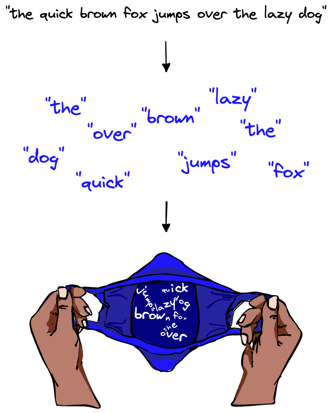
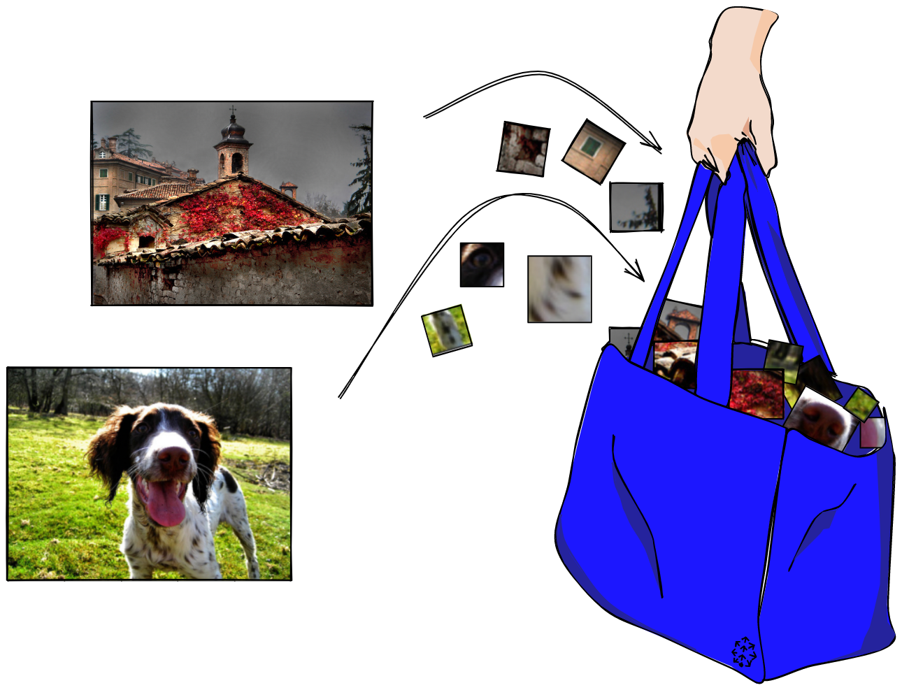
Similarly, in bag of visual words the images are represented by patches, and their unique patterns (or visual features) are extracted from the image.
However, despite the similarity, these visual features are not visual words just yet; we must perform a few more steps. For now, let’s focus on understanding what these visual features are.
Visual features consist of two items:
-
Keypoints are points in an image, which do not change if the image is rotated, expanded, or scaled and
-
Descriptors are vector representations of an image patch found at a given keypoint.
These visual features can be detected and extracted using a feature detector, such as SIFT (Scale Invariant Feature Transform), ORB (Oriented FAST and Rotated BRIEF), or SURF (Speeded Up Robust Features).
The most common is SIFT as it is invariant to scale, rotation, translation, illumination, and blur. SIFT converts each image patch into a $128$-dimensional vector (i.e., the descriptor of the visual feature).
A single image will be represented by many SIFT vectors. The order of these vectors is not important, only their presence within an image.
Codebooks and Visual Words
After extracting visual features we build a codebook, also called a dictionary or vocabulary. This codebook acts as a repository of all existing visual words (similar to an actual dictionary, like the Oxford English Dictionary).
We use this codebook as a way to translate a potentially infinite variation of visual features into a predefined set of visual words.
How? The idea is to group similar visual features into clusters. Each cluster is assigned a central point which represents the visual word translation (or mapping) for that group of visual features. The standard approach for grouping visual features into visual words is k-means clustering.
K-means divides the data into $k$ clusters, where $k$ is chosen by us. Once the data is grouped, k-means calculates the mean for each cluster, i.e., a central point between all of the vectors in a group. That central point is a centroid (i.e., a visual word).
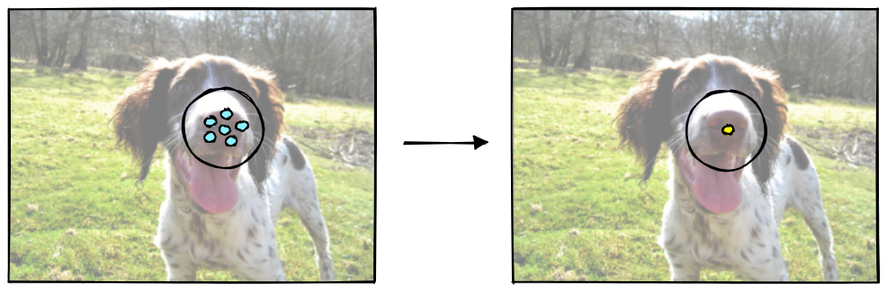
After finding the centroids, k-means iterates through each data point (visual feature) and checks which centroid (visual word) is nearest. If the nearest centroid has changed, the data point switches grouping, being assigned to the new nearest centroid.
This process is repeated over a given number of iterations or until the centroid positions have stabilized.
With that in mind, how do we choose the number of centroids, $k$?
It is more of an art than a science, but there are a few things to consider. Primarily, how many visual words can cover the various relevant visual features in the dataset.
That’s not an easy thing to figure out, and it’s always going to require some guesswork. However, we can think of it using the language equivalent, bag of words.
If our language dataset covered several documents about a specific topic in a single language, we would find fewer unique words than if we had thousands of documents, spanning several languages about a range of topics.
The same is true for images; dogs and/or animals could be a topic, and buildings could be another topic. As for the equivalent of different languages, this is not a perfect metaphor but we could think of different photography styles, drawings, or cartoons. All of these added layers of complexity increase the number of visual words needed to accurately represent the dataset.
Here, we could start with choosing a smaller $k$ value (e.g., $100$ or $150$) and re-run the code multiple times changing $k$ until convergence and/or our model seems to be identifying images well.
If we choose $k=150$, k-means will generate $150$ centroids and, therefore, $150$ visual words.
When we perform the mapping from new visual feature vectors to the nearest centroid (i.e., visual word), we categorize visual features into a more limited set of visual words. This process of reducing the number of possible unique vectors is called vector quantization.
Using a limited set of visual words allows us to compress our image descriptions into a set of visual word IDs. And, more importantly, it helps us represent similar features across images using a shared set of visual words.
That means that the visual words shared by two images of churches may be quite large, meaning they’re similar. However, an image of a church and an image of a dog will share far fewer visual words, meaning they’re dissimilar.
After those steps, our images will be represented by a varying number of visual words. From here we move on to the next step of transforming these visual words into image-level frequency vectors.
Frequency Vectors
We can count the frequency of these visual words and visualize them with histograms.
The x-axis of the histogram is the codebook, while the y-axis is the frequency of each visual word (in the codebook) for that image.
If we consider $2$ images, we can represent the image histograms as follows:
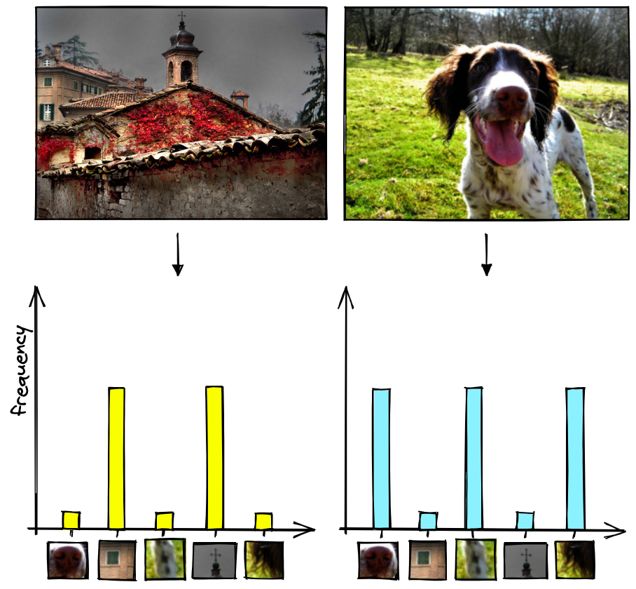
To create these representations, we have converted each image into a sparse vector where each value in the vector represents an item in the codebook (i.e., the x-axis in the histograms). Most of the values in each vector will be zero because most images will only contain a small percentage of total number of visual words, which is why we refer to them as sparse vectors.
As for the non-zero values in our sparse vector, they are calculated in the same way that we calculated our histogram bar heights. They are equal to the frequency of a particular visual word in an image.
This works, but it’s a crude way to create these sparse vector representations. Because many visual words are actually not that important, we add one more step.
Tf-idf
In language there are some words that are more important than others in that they give us more information. If we used the sentence “the history of Rome” to search through a set of articles, the words “the” and “of” should not be given the same importance as “history” or “Rome”.
These less important words are often very common. If we only consider the frequency of words shared with our “the history of Rome” query, the article with the most “the»s could be scored highest.
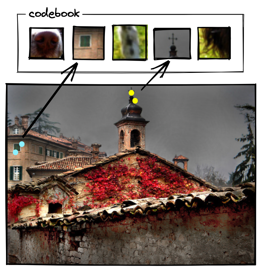
This problem is also found in images. A visual word extracted from a patch of sky in an image is unlikely to tell us whether this image is of a church or a dog. Some visual words are more relevant than others.
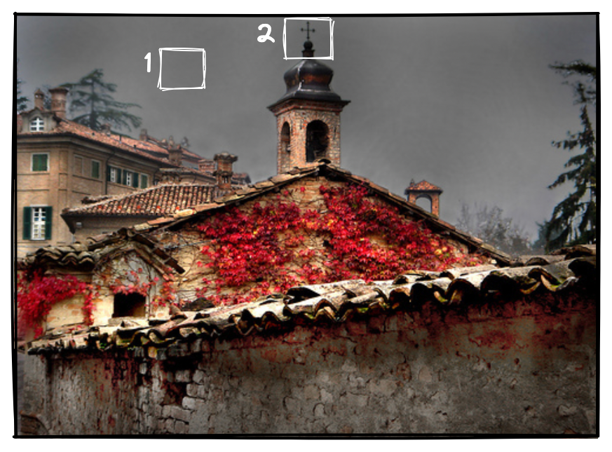
In the example above, we would expect a visual word representing the sky 1 to be less relevant than a visual word representing the cross on top of the bell tower 2.
That is why it is important to adjust the values of our sparse vector to give more weight to more relevant visual words and less weight to less relevant visual words.
To do that, we can use the tf-idf (term-frequency inverse document frequency) formula, which is calculated as follows:
$$
tftextrm{–}idf_{t,d} = tf_{t,d} * idf_t = tf_{t,d} * logfrac{N}{df_t}
$$
Where:
- $tf_{t,d}$ is the term frequency of the visual word $t$ in the image $d$ (the number of times $t$ occurs in $d$),
- $N$ is the total number of images,
- $df_t$ number of images containing visual word $t$,
- $logfrac{N}{df_t}$ measures how common the visual word $t$ is across all images in the database. This is low if the visual word $d$ occurs many times in the image, high otherwise.
After tf-idf, we can visualize the vectors via our histogram again, which will better reflect the image’s features.
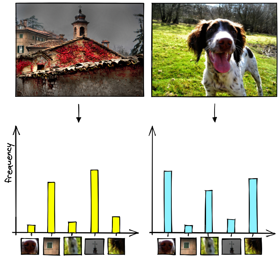
Before we were giving the same importance to image’s patches in an image; now they’re adjusted based on relevance and then normalized.
We’ve now trained our codebook and learned how to process each vector for better relevance and normalization. When wanting to embed new images with this pipeline, we repeat the process but avoid retraining the codebook. Meaning we:
- Extract the visual features,
- Transform them into visual words using the existing codebook,
- Use these visual words to create a sparse frequency vector,
- Adjust the frequency vector based on relevance with tf-idf, giving us our final sparse vector representations.
After that, we’re ready to compare these sparse vectors to find similar or dissimilar images.
Measuring Similarity
There are several metrics we can use to calculate similarity or distance between two vectors. The most common are:
-
Cosine similarity,
-
Euclidean distance, and
-
Dot product similarity.
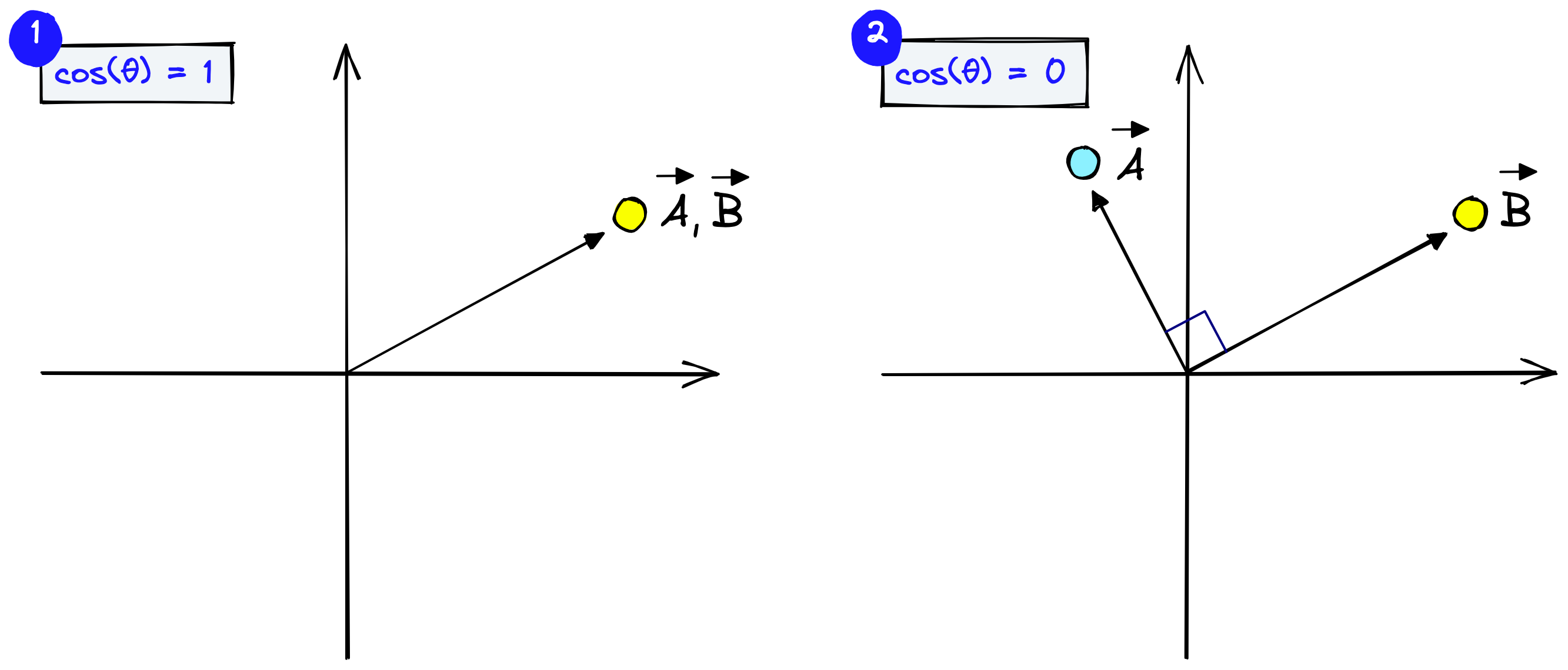
We will use cosine similarity which measures the angle between vectors. Vectors pointing in a similar direction have a lower angular separation and therefore higher cosine similarity.
Cosine similarity is calculated as:
$$
cossim(A,B)= cos(theta)=frac{A cdot B}{||A|| space ||B||}
$$
Cosine similarity generally gives a value ranging $[-1,1]$. However, if we think about the frequency of visual words, we cannot consider them as negative. Therefore, the angle between two term frequency vectors cannot be greater than $90°$, and cosine similarity ranges between $[0,1]$.
It equals $1$ if the vectors are pointing in the same direction (the angle equals $0$) and $0$ if vectors are perpendicular.
If we consider three different images and we build a matrix based on cosine similarity:
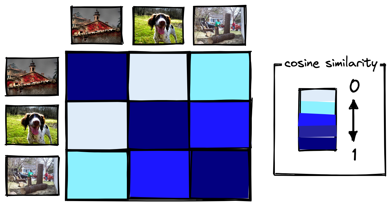
We can see that cosine similarity is $1$ when the image is exactly the same (i.e., in the main diagonal). The cosine similarity approaches $0$ as the images have less in common.
Let’s now move on to implementing bag of visual words with Python.
Implementing Bag of Visual Words
The next section will work through the implementation of everything we’ve just learned in Python. If you’d like to follow along, use this Colab notebook.
Imagenette Dataset Preprocessing
First, we want to import a dataset of images to train the model.
Feel free to use any images you like. However, if you’d like to follow along with the same dataset, we will use the frgfm/imagenette dataset from HuggingFace Datasets.
In[2]:
from datasets import load_dataset

# download the dataset
imagenet = load_dataset(
    'frgfm/imagenette',
    'full_size',
    split='train',
    ignore_verifications=False  # set to True if seeing splits Error
)
imagenet
Out[2]:
Dataset({
features: ['image', 'label'],
num_rows: 9469
})The dataset contains 9469 images, covering a range of images with dogs, radios, fishing, cities, etc. The image feature contains the images themselves stored as PIL object, meaning we can view them in a notebook like so:
In[3]:
# important to use imagenet[0]['image'] rather than imagenet['image'][0]
# as the latter loads the entire image column then extracts index 0 (it's slow)
imagenet[3264]['image']
Out[3]:
In[4]:
imagenet[5874]['image']Out[4]:
To process these images we need to transform them from PIL objects to numpy arrays.
import numpy as np

# initialize list
images_training = []

for n in range(0,len(imagenet)):
    # generate np arrays from the dataset images
    images_training.append(np.array(imagenet[n]['image']))
The dataset mostly consists of color images containing three color channels (red, green, and blue), but some are also grayscale containing just a single channel (brightness). To optimize processing time and keep everything as simple as possible, we will transform color images to grayscale.
import cv2  # pip install opencv-contrib-python opencv-python

# convert images to grayscale
bw_images = []
for img in images_training:
    # if RGB, transform into grayscale
    if len(img.shape) == 3:
        bw_images.append(cv2.cvtColor(img, cv2.COLOR_BGR2GRAY))
    else:
        # if grayscale, do not transform
        bw_images.append(img)
The arrays in bw_images are what we will be using to create our visual features, visual words, frequency vectors, and tf-idf vectors.
Visual Features
With our dataset prepared we’re ready to move on to extracting visual features (both keypoints and descriptors). As mentioned earlier, we will use the SIFT feature detection algorithm.
# defining feature extractor that we want to use (SIFT)
extractor = cv2.xfeatures2d.SIFT_create()

# initialize lists where we will store *all* keypoints and descriptors
keypoints = []
descriptors = []

for img in bw_images:
    # extract keypoints and descriptors for each image
    img_keypoints, img_descriptors = extractor.detectAndCompute(img, None)
    keypoints.append(img_keypoints)
    descriptors.append(img_descriptors)
It’s worth noting that if an image doesn’t have any noticeable features (e.g., it is a flat image without any edges, gradients, etc.), extraction with SIFT can return None. We don’t have that problem with this dataset, but it’s something to watch out for with others.
Now that we have extracted the visual features, we can visualize them with matplotlib.
In[10]:
output_image = []
for x in range(3):
    output_image.append(cv2.drawKeypoints(bw_images[x], keypoints[x], 0, (255, 0, 0),
                                 flags=cv2.DRAW_MATCHES_FLAGS_DRAW_RICH_KEYPOINTS))
    plt.imshow(output_image[x], cmap='gray')
    plt.show()
The centre of each circle is the keypoint location, and the lines from the centre of each circle represent keypoint orientation. The size of each circle is the scale at which the features were detected.
With our visual features ready, we can move onto the next step of creating visual words.
Visual Words and the Codebook
Earlier we described the “codebook”. The codebook acts as a vocabulary where we store all of our visual words. To create the codebook we use k-means clustering to quantize our visual features into a smaller set of visual words.
Our full set of visual features is big, and training k-means with the full set will take some time. So, to avoid that and also emulate a real-world scenario where we are unlikely to train on all images that we’ll ever process, we will use a smaller sample of 1000 images.
# set numpy seed for reproducability
np.random.seed(0)
# select 1000 random image index values
sample_idx = np.random.randint(0, len(imagenet)+1, 1000).tolist()

# extract the sample from descriptors
# (we don't need keypoints)
descriptors_sample = []

for n in sample_idx:
    descriptors_sample.append(np.array(descriptors[n]))
Our descriptors_sample contains a single array for each image, and each array can contain a varying number of SIFT feature vectors. When training k-means, we only care about the feature vectors, we don’t care about which image they’re coming from. So, we need to flatten descriptors_sample into a single array containing all descriptors.
In[13]:
all_descriptors = []
# extract image descriptor lists
for img_descriptors in descriptors_sample:
    # extract specific descriptors within the image
    for descriptor in img_descriptors:
        all_descriptors.append(descriptor)
# convert to single numpy array
all_descriptors = np.stack(all_descriptors)
In[14]:
# check the shape
all_descriptors.shape
From this, we get all_descriptors, a single array containing all feature vectors from our sample. There are ~1.3M of these.
We now want to group similar visual features (descriptors) using k-means. After a few tests, we chose $k=200$ for our model.
After k-means, all images will have been reduced to visual words, and the full set of these visual words become our codebook.
# perform k-means clustering to build the codebook
from scipy.cluster.vq import kmeans

k = 200
iters = 1
codebook, variance = kmeans(all_descriptors, k, iters)
Once built, the codebook does not change. No matter how many more visual features we process, no more visual words are added as we will use it solely as a mapping between new visual features and the existing visual words.
It can be difficult to find the optimal size of our codebook — if too small, visual words could be unrepresentative of all image regions, and if too large, there could be too many visual words with little to no of them being shared between images (making comparisons very hard or impossible).
With our codebook complete, we can use it to transform the full dataset of visual features into visual words.
In[19]:
# vector quantization
from scipy.cluster.vq import vq

visual_words = []
for img_descriptors in descriptors:
    # for each image, map each descriptor to the nearest codebook entry
    img_visual_words, distance = vq(img_descriptors, codebook)
    visual_words.append(img_visual_words)
In[20]:
# let's see what the visual words look like for image 0
visual_words[0][:5], len(visual_words[0])
Out[20]:
(array([ 84, 22, 45, 172, 172], dtype=int32), 397)In[21]:
# the centroid that represents visual word 84 is of dimensionality...
codebook[84].shape  # (all have the same dimensionality)
We can see here that image 0 contains 397 visual words; the first five of those are represented by [84, 22, 45, 172, 172], which are the index values of the visual word vector found in the codebook. This visual word vector shares the same dimensionality as our SIFT feature vectors because it represents a cluster centroid from those feature vectors.
Sparse Frequency Vectors
After building our codebook and creating our image representations with visual words, we can move on to building sparse vector representations from these visual words.
We do this to compress the many visual word vectors representing our images into a single vector of set dimensionality. By doing this, we are able to directly compare our image representations using metrics like cosine similarity and Euclidean distance.
To create these frequency vectors, we look at how many times each visual word is found in an image. There are only 200 unique visual words (the length of our codebook), so each of these frequency vectors will have dimensionality 200, where each value becomes a count for a specific visual word.
In[22]:
frequency_vectors = []
for img_visual_words in visual_words:
    # create a frequency vector for each image
    img_frequency_vector = np.zeros(k)
    for word in img_visual_words:
        img_frequency_vector[word] += 1
    frequency_vectors.append(img_frequency_vector)
# stack together in numpy array
frequency_vectors = np.stack(frequency_vectors)
In[23]:
frequency_vectors.shapeAfter creating the frequency vectors, we’re left with a single vector representation for each image. We can see an example of the frequency vector for image 0 below:
In[45]:
# we know from above that ids 84, 22, 45, and 172 appear in image 0
for i in [84,  22,  45, 172]:
    print(f"{i}: {frequency_vectors[0][i]}")
Out[45]:
84: 2.0
22: 2.0
45: 3.0
172: 4.0
In[25]:
frequency_vectors[0][:20]Out[25]:
array([0., 0., 2., 0., 2., 1., 0., 3., 1., 0., 0., 0., 5., 3., 4., 0., 1.,
0., 0., 0.])In[26]:
# visualize the frequency vector for image 0
plt.bar(list(range(k)), frequency_vectors[0])
plt.show()
Out[26]:
Tf-idf
Our frequency vector can already be used for comparing images using our similarity and distance metrics. However, it is not ideal as it does not consider the different levels of relevance of each visual word. So, we must use tf-idf to adjust the frequency vector to consider relevance.
$$
tftextrm{-}idf_{t,d} = tf_{t,d} * idf_t = tf_{t,d} * logfrac{N}{df_t}
$$
We first calculate $N$ and $df_t$, both of which are shared across the entire dataset as the image $d$ is not considered by either parameter. Naturally, $idf_t$ also produces a single vector shared by the full dataset.
In[27]:
# N is the number of images, i.e. the size of the dataset
N = 9469

# df is the number of images that a visual word appears in
# we calculate it by counting non-zero values as 1 and summing
df = np.sum(frequency_vectors > 0, axis=0)
Out[28]:
((200,), array([7935, 7373, 7869, 8106, 7320]))In[29]:
idf = np.log(N/ df)
idf.shape, idf[:5]
Out[29]:
((200,), array([0.17673995, 0.25019863, 0.18509232, 0.15541878, 0.25741298]))With $idf_t$ calculated, we just need to multiply it by each $tf_{t,d}$ vector to get our $tf textrm{-} idf_{t,d}$ vectors. Fortunately, we already have the $tf_{t,d}$ vectors, as they are our frequency vectors.
In[30]:
tfidf = frequency_vectors * idf
tfidf.shape, tfidf[0][:5]
Out[30]:
((9469, 200),
array([0. , 0. , 0.37018463, 0. , 0.51482595]))In[31]:
# we can visualize the histogram for image 0 again
plt.bar(list(range(k)), tfidf[0])
plt.show()
Out[31]:
We now have 9469 200-dimensional sparse vector representations of our images.
Search
These sparse vectors have been built in such a way that images that share many similar visual features should share similar sparse vectors. We can use cosine similarity to compare these images and identify similar images.
We will start by searching with image 1200:

In[41]:
from numpy.linalg import norm

top_k = 5
i = 1200

# get search image vector
a = tfidf[i]
b = tfidf  # set search space to the full sample
# get the cosine distance for the search image `a`
cosine_similarity = np.dot(a, b.T)/(norm(a) * norm(b, axis=1))
# get the top k indices for most similar vecs
idx = np.argsort(-cosine_similarity)[:top_k]
# display the results
for i in idx:
    print(f"{i}: {round(cosine_similarity[i], 4)}")
    plt.imshow(bw_images[i], cmap='gray')
    plt.show()
Out[41]:
1200: 1.0
1609: 0.944
1739: 0.9397
4722: 0.9346
7381: 0.9304
The top image is of course the same image; as they are exact matches we can see the expected cosine similarity score of 1.0. Following this, we have two highly similar results. Interestingly, the fourth image seems to have been pulled through due to similarity in background foliage.
Here are a few more sets of results, showing the varied performance of the approach with different items.
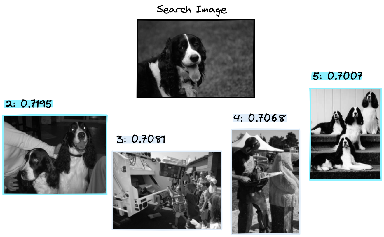
Here we get a good first result, followed by irrelevant images and a final good result in fifth position, a 50% success rate.
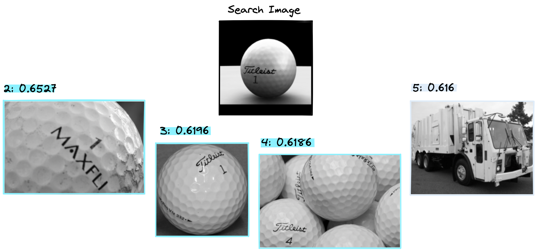
Bag of visual words seems to work well with golf balls, identifying 3/4 of relevant images.
If you’re interested in seeing more results, check out the Colab notebook here.
That’s it for this article on bag of visual words, one of the most successful methods for image classification and retrieval without the use of neural networks or other deep learning methods.
One great aspect of this approach is that it is fairly reliable and interpretable. There is no black box of AI here, so when applied to a lot of data we will rarely get too many surprising results.
We know that images with similar edges, textures, and colors are likely to be identified as similar; the features being identified are set by the SIFT (or other) algorithms.
All of this makes bag of visual words a good option for image retrieval or classification, where we need to focus on the features that we know algorithms like SIFT can deal with, i.e. we’re focused on finding similar object edges (that are resistant to scale, noise, and illumination changes). Finally, these well-defined algorithms give us a huge advantage when interpretability is important.
Resources
Code Notebook, GitHub Examples Repo
Next Chapter:
AlexNet and ImageNet: The Birth of Deep Learning
- 15 min read
- Data Visualization,
Design,
UX,
Guides
Data visualizations are everywhere; from the news to the nutritional info on cereal boxes, we’re constantly being presented with graphical representations of data. Why? Data visualization is a method of communication. Using the right type can help you quickly convey nuanced information to your audience in a visually appealing way. However, the diversity of styles used in both digital and print formats can be overwhelming. In this article, we will break down the most common visualization types to help guide you through selecting the best choice for your specific needs.
Before getting into the content of the article, let’s briefly address language usage. “Graph” and “chart” are often used interchangeably, but specificity is important. In this article, the term “graph” refers to visual representations of data on a Cartesian plane (they often look like a grid and have an x-, y-, and sometimes z-axis). “Chart” is used as a catchall word for visual representations of data. It’s like the relationship between squares (graphs) and rectangles (charts); all graphs are charts, but not all charts are graphs.
With this understanding, we can dive into the considerations involved in selecting a chart type.
How To Choose The Right Chart Type
There are some questions you should consider when choosing the right data visualization for your purposes, and we’ll dive into each of these in turn:
- What message am I trying to communicate with the data?
- What is the purpose of the data visualization?
- Who is the audience?
- What type and size of data set am I working with?
What Message Am I Trying To Communicate With The Data?
Each data visualization should have a primary message. Having a clear idea of what you want to communicate and focusing on that will increase the overall quality of your data visualization, and it will help you narrow down chart types based on the complexity of the message and/or the amount of information being communicated.
For instance, sometimes, a simple table is enough to communicate a singular idea. However, if the message is more complex and/or meant to empower or motivate the audience to take action, it is worth thinking about more dynamic chart types. The following example of this guidance is based on a dataset created by Stetson Done on Kaggle.
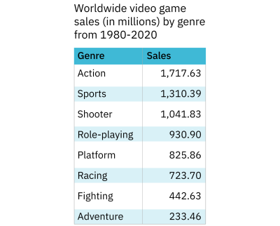
The pared-down dataset is shown as a table. In one column, there’s a categorical variable (genre) and in the other is a quantitative variable (sales). The categories are sorted by sales rather than alphabetically by genre. This makes it easy to glance at the table and get an idea of what the most popular genres are. As an added bonus, the table takes up relatively little space. If the purpose of the data visualization is to communicate simple information about the popularity of various video game genres from 1980-2020, the table in Figure 1 is a good choice. But what if the information is more complex?
The following chart shows a table created with the same dataset but which shows slightly different information. Instead of eight genres, this table shows five, and instead of the total worldwide sales for each genre, it presents sales figures for two regions: the European Union and North America. The message this table is trying to communicate is twofold: the data speaks to the sales of various video game genres in two regions and presents a comparison of the sales across these two regions.
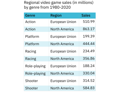
In this format, comparing sales for a genre between the two regions is very straightforward. However, comparing sales across all genres for each region is more complicated. The result is that the latter part of the message isn’t being communicated as effectively.
By changing the type of data visualization we use, we can effectively communicate more information. The following figure displays the same data and the table but in the form of a grouped bar graph.

The bar graph allows the audience to compare each genre across the two regions and to compare sales of all the genres for each region. Because the bar graph communicates more information than the table in Figure 2, it’s a better choice for this data.
Keep in mind that less is more. When selecting a chart type, try to create a data visualization that’s as simple as possible while effectively communicating your intended message(s) to your audience.
More after jump! Continue reading below ↓
What Is The Purpose Of The Data Visualization?
In the field of data visualization, there are four largely accepted categories of data visualization that relate to different purposes:
- Comparison
- Composition
- Distribution
- Relationship
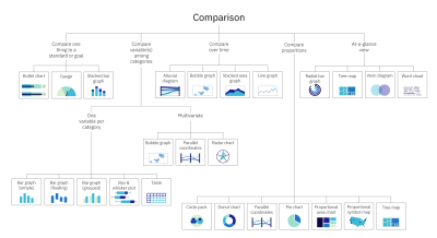
Comparison
How are the elements similar or different? This can be among items and/or over time.
Example: Comparing the sales of two different brands of dog food in a single retail location.
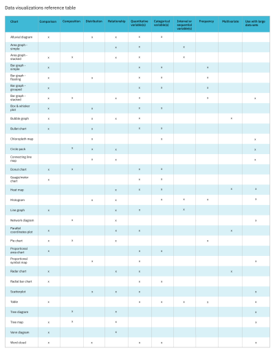
Comparison charts include alluvial diagrams, area graphs (stacked), bar graphs (simple, floating, grouped, and stacked), box and whisker plots, bubble graphs, bullet charts, donut charts, gauge charts, line graphs, parallel coordinates, pie charts, proportional area charts, proportional symbol maps, radar charts, radial bar charts, tree maps, Venn diagrams, and word clouds. To learn more about each of these charts, check out the Chart reference guide, one of two resources provided as a companion to this article.
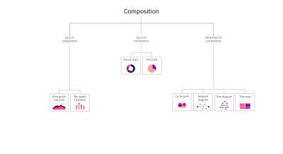
Composition
What parts make up the whole? The composition can be static or change over time.
Example: Showing the breakdown of the diet of Pallas cats.
Composition charts include area graphs (stacked), bar graphs (stacked), circle packs, donut charts, network diagrams, pie charts, tree diagrams, and tree maps. To learn more about each of these charts, check out the Chart reference guide.
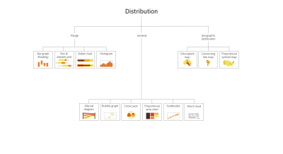
Distribution
Where do the values in a data set fall? Are there outliers?
Example: Communicating the distribution of grades within a middle school class, including the average and outliers.
Distribution charts include alluvial diagrams, bar graphs (floating), box and whisker plots, bubble graphs, bullet charts, circle packs, choropleth maps, connecting line maps, histograms, proportional area charts, proportional symbol maps, scatterplots, and word clouds. To learn more about each of these charts, check out the Chart reference guide.
Relationship
How do the elements relate to each other? Is there a correlation?
Example: Showing how colder temperatures are correlated to fewer ice cream sales.
Relationship charts include alluvial diagrams, bubble graphs, circle packs, connecting line maps, heat maps, histograms, line graphs, network diagrams, parallel coordinates, radar charts, scatterplots, tree diagrams, and venn diagrams. To learn more about each of these charts, check out the Chart reference guide.
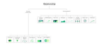
Some chart types fall into multiple categories. For instance, tree diagrams can provide information both on what elements make up a category and on the relationships between those elements. A classic example is a site map. Site maps communicate a list of the pages within a site (composition) and the relationships between the pages.
A donut chart is another good example. Figure 5 shows the results of a second-grade class being asked what their favorite animal is.
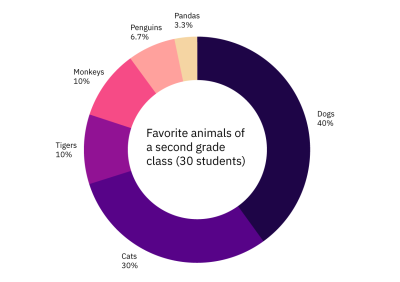
Not only does Figure 5 give you a complete listing of the favorite animals selected by the class, but it also allows you to compare the popularity of those animals. Thus, it achieves both comparison and composition.
Multi-purpose charts don’t have to be used for multiple purposes, but when you do want a single chart that can do more than one thing, these types of charts can be a good choice. You can learn more about which chart types are multi-purpose, including what types of variables they use in the Data visualizations table, one of two resources provided as a companion to this article (reference Figure 12).
Knowing what the purpose of the data visualization is will help narrow the options down significantly. If you find that you have multiple purposes and/or messages that can’t be communicated in a single multi-purpose chart, consider using multiple charts, especially if your audience is less familiar with data visualizations and may have trouble reading a more complex chart type. For more information on different chart types, including their purpose, when to use each, and an example, refer to the Chart reference guide.
That brings us to the next consideration in choosing a chart type — audience.
Who Is The Audience?
Knowing your audience is key to effective communication. For our purposes, knowledge about your audience will be immensely helpful in both selecting the type of data visualization you’ll use as well as deciding various aspects of the design.
When considering your audience, it’s important to think about things like:
- How familiar they are with the subject matter of your data.
- How much context they already have versus what you should supply.
- Their familiarity with various methods of data visualization.
This information should help inform your selection of chart type. For instance, some data visualization types are quite complex and should only be used with high-level experts in the field and/or individuals who are very familiar with data visualizations. For more information on which chart should only be used with this type of audience, refer to the “When to use” sections of the reference guide. The following is an example of one set of data communicated with two different chart types.
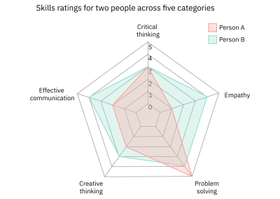
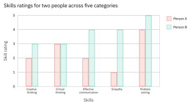
Both charts communicate the same skill ratings for two individuals across five categories. Figure 6 uses a radar chart. While these can be a good tool to communicate comparative data, many audiences aren’t familiar with this chart type or with the circular format in which they present the data. As such, Figure 6 may be more difficult for many people to read than Figure 7.
Figure 7, on the other hand, uses a grouped bar graph to display the same data. Since grouped bar graphs are familiar to most people regardless of their familiarity with data visualization, it’s more likely to be easier to understand by a larger audience.
If you’re wondering, “Why not always opt for the simpler chart type,” you’re not alone. Simplicity is key, but it should be looked at from the perspective of the bigger picture. Some chart types, while more complicated for a general lay audience to understand, communicate information more successfully for audiences that are familiar with them. This is evident in Figures 6 and 7. While radar charts are likely more difficult for a random person to read, in this case, the radar chart, for someone who can easily read it, does a better job of allowing for a comparison across the two people.
Considering your audience will be important after you’ve selected your chart type as well. For a general audience — not composed of experts — you should use simple, straightforward language and avoid using jargon or technical terminology. Additionally, for general audiences without a lot of background knowledge on the topic of your data, you may want to include more contextual information before introducing the data visualization or provide context and additional information within the visualization.
A stacked area graph is a good example of this. Stacked area graphs are like simple area graphs. The difference is that they show two or more data series stacked on one another. Each data series after the first one starts where the one before it ends. In other words, if point A for data series 1 stops at $18 million, then point A for data series 2 will begin at $18 million.
For this reason, they can be a bit confusing if you’re not familiar with them, and if they aren’t labeled, reading them can require some math. However, the benefit of using them is that they show the values for each series as well as the totals (for each point, the top of the stack is the total). Figures 8 and 9 demonstrate this.
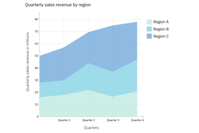
 Stacked area graph: Quarterly sales revenue. (Large preview)
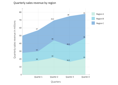
Both Figures 8 and 9 show a stacked area graph with the same data. However, Figure 9 provides additional information by labeling the values for each region for each quarter. This not only eliminates the need for the audience to calculate the figures, but it also helps to illuminate a characteristic of stacked area graphs. Because of the way they’re laid out, it can be difficult to compare the values for the different data series (in this case, regions) at a single point, for instance, Quarter 1. Adding the values to the graph helps with that. However, it’s not always a good idea to label every element in a graph. Doing so with large data sets often results in a graph that’s overcrowded and harder to read (see Figure 10).
By this point, the types of charts still under consideration should have narrowed significantly based on your message, purpose, and audience. Based on your remaining options, it’s now largely a matter of matching up the details of your data set, including the type and number of variables for the remaining options.
What Type And Size Of Data Am I Working With?
There are different types of data and variables:
- Quantitative: numerical (like population size or temperature).
- Continuous: numerical data can take any value between two numbers (ex: weight or temperature).
- Discrete: numerical data that, unlike continuous data, has a limited number of possible values and includes finite, numeric, countable, non-negative integers (ex: the number of people who have been to space).
- Ordinal: non-numerical data that has a natural order (ex: days of the week or spiciness levels on a menu (mild, spicy, very spicy)).
- Categorical (aka nominal): categories that don’t have an inherent order or numerical values (ex: oak, ash, and elm trees; pink, purple, and blue).
Knowing what type of data you plan to use in your data visualization will help you eliminate some chart types. For instance, if your data consists of a categorical and a quantitative variable, you can’t use a histogram because they show frequency and quantitative variables split into intervals.
Similarly, the size of your data set can help you to eliminate some chart types. Certain data visualization types like bar graphs and pie charts only lend themselves to being used with a small set of data. The reason is that charts should communicate a message in a way that’s easy to understand. A bar graph with eighteen bars or a pie chart with twenty slices is not going to be easy to read. However, there are chart types that can be used with large data sets. Figures 10 and 11 demonstrate this.
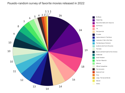
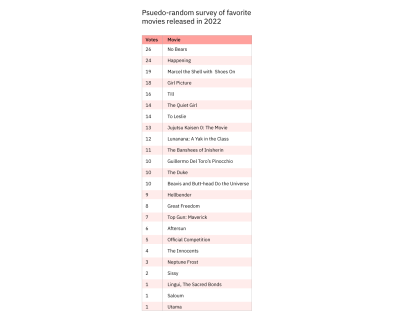
Both charts are based on the same data, but when presented as a pie chart, the information takes longer to process than when presented in a table. Because the pie chart has so many slices, it’s not possible to label each one with the movie title, so we have to use a key. This means that the audience will have to keep scanning from right to left over and over again to look from the key to the pie chart. The table, on the other hand, has the number of votes presented beside the movie title, making it easy to understand not only the popularity of the movies but the exact number of votes each one received.
For more information on which charts work with large data sets and other information about over 30 of the most popular chart types, refer to Figure 12.
Conclusion
We’ve covered the most important considerations when choosing a chart type, as well as what to look out for. To learn more about data visualizations, refer to the resources linked at the bottom of the article.
Hopefully, you now feel empowered with the knowledge you need to create a stellar data visualization! If you want to try out some of the tips in the article and don’t have a data set to work with, you can browse sites like Kaggle, World Bank Open Data, and Google Public Data Explorer. As a final reminder, keep it simple and focus on your message — you’ve got this!
Resources
- Chart Reference Guide
- Data Visualizations Table
General Info
- The Data Visualisation Catalogue
- Data Viz Project
- Interaction Design Foundation, Data Visualization
Narratives And Data Visualization
- “Designing experiences through data stories”, Marion Hekeler
- “Data Storytelling: How to Effectively Tell a Story with Data”, Catherine Cote
How To Choose A Chart
- The Extreme Presentation Method
- “Data Visualization 101: How to Choose a Chart Type”, Sara A. Metwalli
- From Data to Viz
- “How to Choose the Right Data Visualization”, Mike Yi, Mel Restori
Design Tips For Data Visualizations
- “Data Visualization Tips For More Effective And Engaging Design”, Tableau
- “Which fonts to use for your charts and tables”, Lisa Charlotte Muth
Data Visualization Inspiration
- The Pudding
- Dataviz Inspiration
- Datawrapper River
- Flowing Data
Ethics And Data
- “The Ethics of Data Visualization”, Peter Haferl
- “Bad Data Visualizations: 5 Examples of Misleading Data”, Tim Stobierski
- “Ethical Data Viz”, Jo Hardin
- Inculcating ethics in data visualization dashboards, Abhinay Gupta Somisetty (Thesis)
![]()
(ah, yk, il)
Filters
Filter by Part of speech
noun
phrase
Suggest
If you know synonyms for Visual representation, then you can share it or put your rating in listed similar words.
Suggest synonym
Menu
Visual representation Thesaurus
External Links
Other usefull source with synonyms of this word:
![]() Synonym.tech
Synonym.tech
![]() Thesaurus.com
Thesaurus.com
Image search results for Visual representation


Cite this Source
- APA
- MLA
- CMS
Synonyms for Visual representation. (2016). Retrieved 2023, April 14, from https://thesaurus.plus/synonyms/visual_representation
Synonyms for Visual representation. N.p., 2016. Web. 14 Apr. 2023. <https://thesaurus.plus/synonyms/visual_representation>.
Synonyms for Visual representation. 2016. Accessed April 14, 2023. https://thesaurus.plus/synonyms/visual_representation.

Wiki User
∙ 5y ago
Want this question answered?
Be notified when an answer is posted
Study guides
Add your answer:
![]() Earn +
Earn +
20
pts
Q: What is another word for visual representations?
Write your answer…
Submit
Still have questions?
![]()
![]()
Related questions
People also asked
In a previous post, we explored techniques for visualizing high-dimensional data. Trying to visualize high dimensional data is, by itself, very interesting, but my real goal is something else. I think these techniques form a set of basic building blocks to try and understand machine learning, and specifically to understand the internal operations of deep neural networks.
Deep neural networks are an approach to machine learning that has revolutionized computer vision and speech recognition in the last few years, blowing the previous state of the art results out of the water. They’ve also brought promising results to many other areas, including language understanding and machine translation. Despite this, it remains challenging to understand what, exactly, these networks are doing.
I think that dimensionality reduction, thoughtfully applied, can give us a lot of traction on understanding neural networks.
Understanding neural networks is just scratching the surface, however, because understanding the network is fundamentally tied to understanding the data it operates on. The combination of neural networks and dimensionality reduction turns out to be a very interesting tool for visualizing high-dimensional data – a much more powerful tool than dimensionality reduction on its own.
As we dig into this, we’ll observe what I believe to be an important connection between neural networks, visualization, and user interface.
Neural Networks Transform Space
Not all neural networks are hard to understand. In fact, low-dimensional neural networks – networks which have only two or three neurons in each layer – are quite easy to understand.
Consider the following dataset, consisting of two curves on the plane. Given a point on one of the curves, our network should predict which curve it came from.
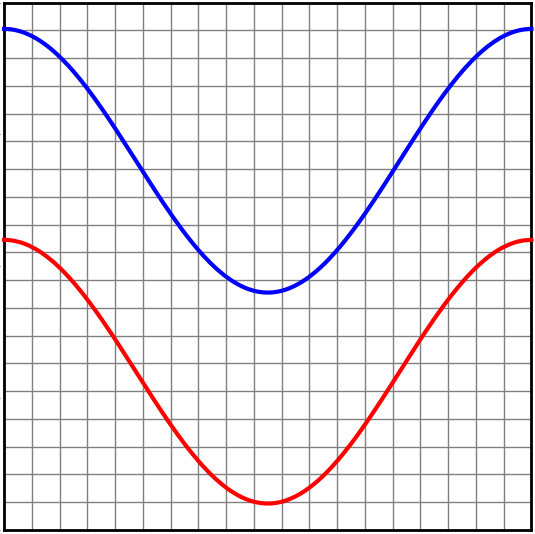
A network with just an input layer and an output layer tries to divide the two classes with a straight line.
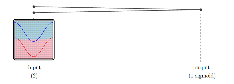
In the case of this dataset, it is not possible to classify it perfectly by dividing it with a straight line. And so, a network with only an input layer and an output layer can not classify it perfectly.
But, in practice, neural networks have additional layers in the middle, called “hidden” layers. These layers warp and reshape the data to make it easier to classify.
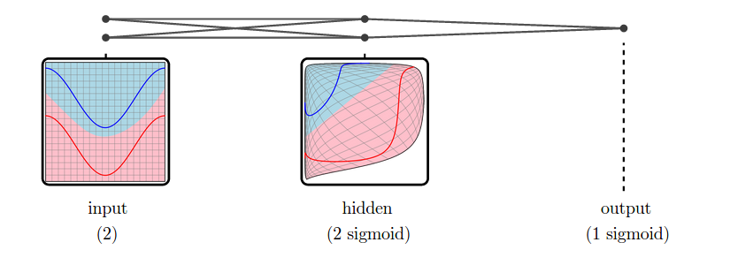
We call the versions of the data corresponding to different layers representations.1 The input layer’s representation is the raw data. The middle “hidden” layer’s representation is a warped, easier to classify, version of the raw data.
Low-dimensional neural networks are really easy to reason about because we can just look at their representations, and at how one representation transforms into another. If we have a question about what it is doing, we can just look. (There’s quite a bit we can learn from low-dimensional neural networks, as explored in my post Neural Networks, Manifolds, and Topology.)
Unfortunately, neural networks are usually not low-dimensional. The strength of neural networks is classifying high-dimensional data, like computer vision data, which often has tens or hundreds of thousands of dimensions. The hidden representations we learn are also of very high dimensionality.
For example, suppose we are trying to classify MNIST. The input representation, MNIST, is a collection of 784-dimensional vectors! And, even for a very simple network, we’ll have a high-dimensional hidden representation. To be concrete, let’s use one hidden layer with a hundred sigmoid neurons.
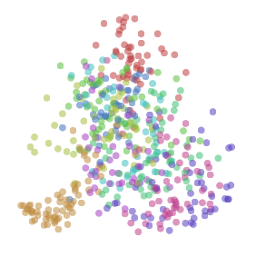
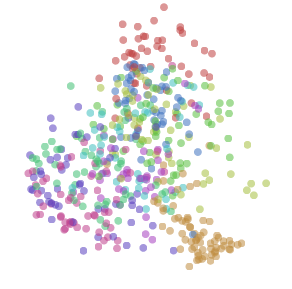
While we can’t visualize the high-dimensional representations directly, we can visualize them using dimensionality reduction. Below, we look at nearest neighbor graphs of MNIST in its raw form and in a hidden representation from a trained MNIST network.
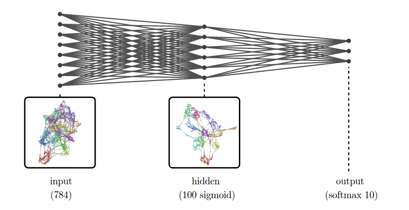
At the input layer, the classes are quite tangled. But, by the next layer, because the model has been trained to distinguish the digit classes, the hidden layer has learned to transform the data into a new representation in which the digit classes are much more separated.
This approach, visualizing high-dimensional representations using dimensionality reduction, is an extremely broadly applicable technique for inspecting models in deep learning.
In addition to helping us understand what a neural network is doing, inspecting representations allows us to understand the data itself. Even with sophisticated dimensionality reduction techniques, lots of real world data is incomprehensible – its structure is too complicated and chaotic. But higher level representations tend to be simpler and calmer, and much easier for humans to understand.
(To be clear, using dimensionality reduction on representations isn’t novel. In fact, they’ve become fairly common. One really beautiful example is Andrej Karpathy’s visualizations of a high-level ImageNet representation. My contribution here isn’t the basic idea, but taking it really seriously and seeing where it goes.)
Example 1: Word Embeddings
Word embeddings are a remarkable kind of representation. They form when we try to solve language tasks with neural networks.
For these tasks, the input to the network is typically a word, or multiple words. Each word can be thought of as a unit vector in a ridiculously high-dimensional space, with each dimension corresponding to a word in the vocabulary. The network warps and compresses this space, mapping words into a couple hundred dimensions. This is called a word embedding.
In a word embedding, every word is a couple hundred dimensional vector. These vectors have some really nice properties. The property we will visualize here is that words with similar meanings are close together.
(These embeddings have lots of other interesting properties, besides proximity. For example, directions in the embedding space seems to have semantic meaning. Further, difference vectors between words seem to encode analogies. For example, the difference between woman and man is approximately the same as the difference between queen and king: (v(«text{woman}!») — v(«text{man}!») ~simeq) (v(«text{queen}!») — v(«text{king}!»)). For more on word embeddings, see my post Deep Learning, NLP, and Representations.)
To visualize the word embedding in two dimensions, we need to choose a dimensionality reduction technique to use. t-SNE optimizes for keeping points close to their neighbors, so it is the natural tool if we want to visualize which words are close together in our word embedding.
Examining the t-SNE plot, we see that neighboring words tend to be related. But there’s so many words! To get a higher-level view, lets highlight a few kinds of words.2 We can see areas corresponding to cities, food, body parts, feelings, relatives and different “travel” verbs.
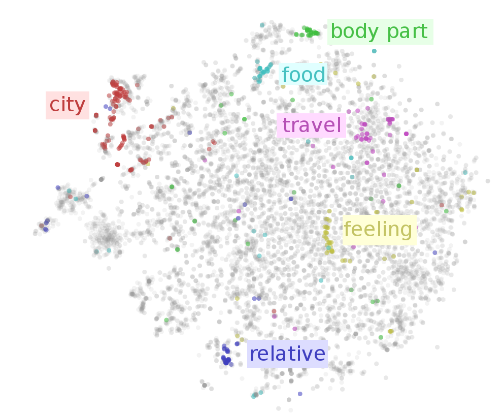
That’s just scratching the surface. In the following interactive visualization, you can choose lots of different categories to color the words by. You can also inspect points individually by hovering over them, revealing the corresponding word.
Color words by WordNet synset (eg. region.n.03):
Looking at the above visualization, we can see lots of clusters, from broad clusters like regions (region.n.03) and people (person.n.01), to smaller ones like body parts (body_part.n.01), units of distance (linear_unit.n.01) and food (food.n.01). The network successfully learned to put similar words close together.
Example 2: Paragraph Vectors of Wikipedia
Paragraph vectors, introduced by Le & Mikolov (2014), are vectors that represent chunks of text. Paragraph vectors come in a few variations but the simplest one, which we are using here, is basically some really nice features on top of a bag of words representation.
With word embeddings, we learn vectors in order to solve a language task involving the word. With paragraph vectors, we learn vectors in order to predict which words are in a paragraph.
Concretely, the neural network learns a low-dimensional approximation of word statistics for different paragraphs. In the hidden representation of this neural network, we get vectors representing each paragraph. These vectors have nice properties, in particular that similar paragraphs are close together.
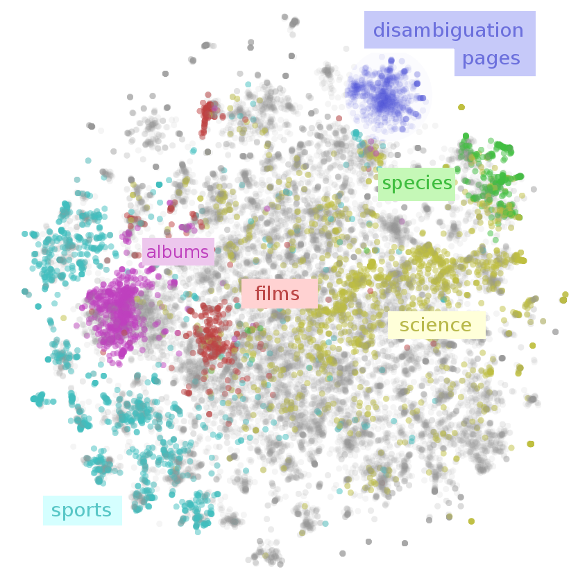
Now, Google has some pretty awesome people. Andrew Dai, Quoc Le, and Greg Corrado decided to create paragraph vectors for some very interesting data sets. One of those was Wikipedia, creating a vector for every English Wikipedia article. I was lucky enough to be there at the time, and make some neat visualizations. (See Dai, et al. (2014))
Since there are a very large number of Wikipedia articles, we visualize a random subset. Again, we use t-SNE, because we want to understand what is close together.
The result is that we get a visualization of the entirety of Wikipedia. A map of Wikipedia. A large fraction of Wikipedia’s articles fall into a few broad topics: sports, music (songs and albums), films, species, and science. I wouldn’t have guessed that! Why, for example, is sports so massive? Well, it seems like many individual athletes, teams, stadiums, seasons, tournaments and games end up with their own articles – that adds up to a lot of articles! Similar reasons lead to the large music, films and species clusters.
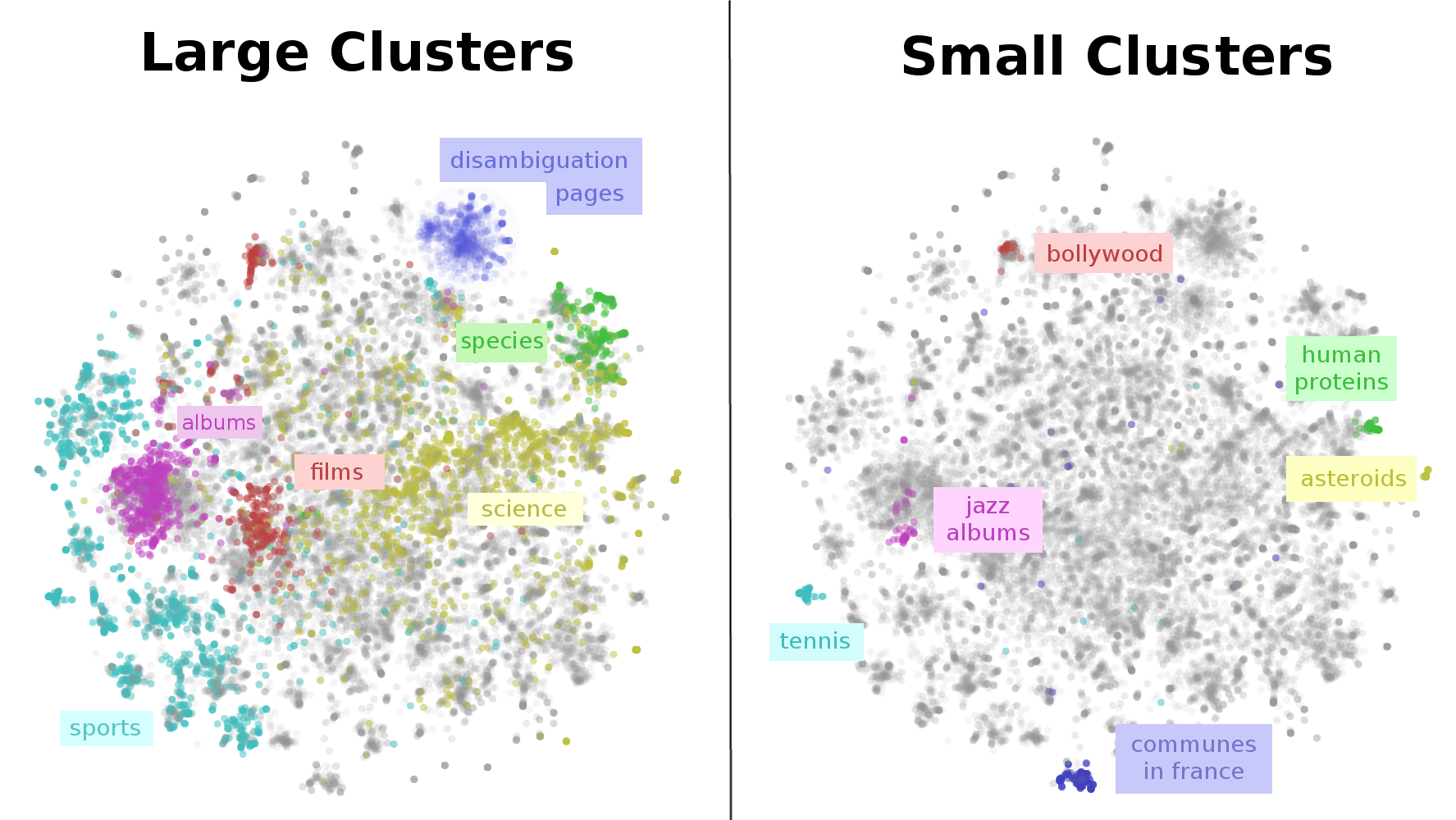
This map of Wikipedia presents important structure on multiple scales. While, there is a large cluster for sports, there are sub-clusters for individual sports like tennis. Films have a separate cluster for non-Western films, like bollywood. Even very fine grained topics, like human proteins, are separated out!
Again, this is only scratching the surface. In the following interactive visualization, you can explore for your self. You can color points by their Wikipedia categories, or inspect individual points by hovering to see the article title. Clicking on a point will open the article.
Color articles by Wikipedia category (eg. films):
Wikipedia Paragraph Vectors Visualized with t-SNE
(Hover over a point to see the title. Click to open article.)
(See this with 50,000 points!)
(Note: Wikipedia categories can be quite unintuitive and much broader than you expect. For example, every human is included in the category applied ethics because humans are in people which is in personhood which is in issues in ethics which is in applied ethics.)
Example 3: Translation Model
The previous two examples have been, while fun, kind of strange. They were both produced by networks doing simple contrived tasks that we don’t actually care about, with the goal of creating nice representations. The representations they produce are really cool and useful… But they don’t do too much to validate our approach to understanding neural networks.
Let’s look at a cutting edge network doing a real task: translating English to French.
Sutskever et al. (2014) translate English sentences into French sentences using two recurrent neural networks. The first consumes the English sentence, word by word, to produce a representation of it, and the second takes the representation of the English sentence and sequentially outputs translated words. The two are jointly trained, and use a multilayered Long Short Term Memory architecture.3
![]()
We can look at the representation right after the English “end of sentence” (EOS) symbol to get a representation of the English sentence. This representation is actually quite a remarkable thing. Somehow, from an English sentence, we’ve formed a vector that encodes the information we need to create a French version of that sentence.
Let’s give this representation a closer look with t-SNE.
Color sentences by first word (eg. The):
Translation representation of sentences visualized with t-SNE
(Hover over a point to see the sentence.)
This visualization revealed something that was fairly surprising to us: the representation is dominated by the first word.
If you look carefully, there’s a bit more structure than just that. In some places, we can see subclusters corresponding to the second word (for example, in the quotes cluster, we see subclusters for “I” and “We”). In other places we can see sentences with similar first words mix together (eg. “This” and “That”). But by and large, the sentence representation is controlled by the first word.
There are a few reasons this might be the case. The first is that, at the point we grab this representation, the network is giving the first translated word, and so the representation may strongly emphasize the information it needs at that instant. It’s also possible that the first word is much harder than the other words to translate because, for the other words, it is allowed to know what the previous word in the translation was and can kind of Markov chain along.
Still, while there are reasons for this to be the case, it was pretty surprising. I think there must be lots of cases like this, where a quick visualization would reveal surprising insights into the models we work with. But, because visualization is inconvenient, we don’t end up seeing them.
Aside: Patterns for Visualizing High-Dimensional Data
There are a lot of established best practices for visualizing low dimensional data. Many of these are even taught in school. “Label your axes.” “Put units on the axes.” And so on. These are excellent practices for visualizing and communicating low-dimensional data.
Unfortunately, they aren’t as helpful when we visualize high-dimensional data. Label the axes of a t-SNE plot? The axes don’t really have any meaning, nor are the units very meaningful. The only really meaningful thing, in a t-SNE plot, is which points are close together.
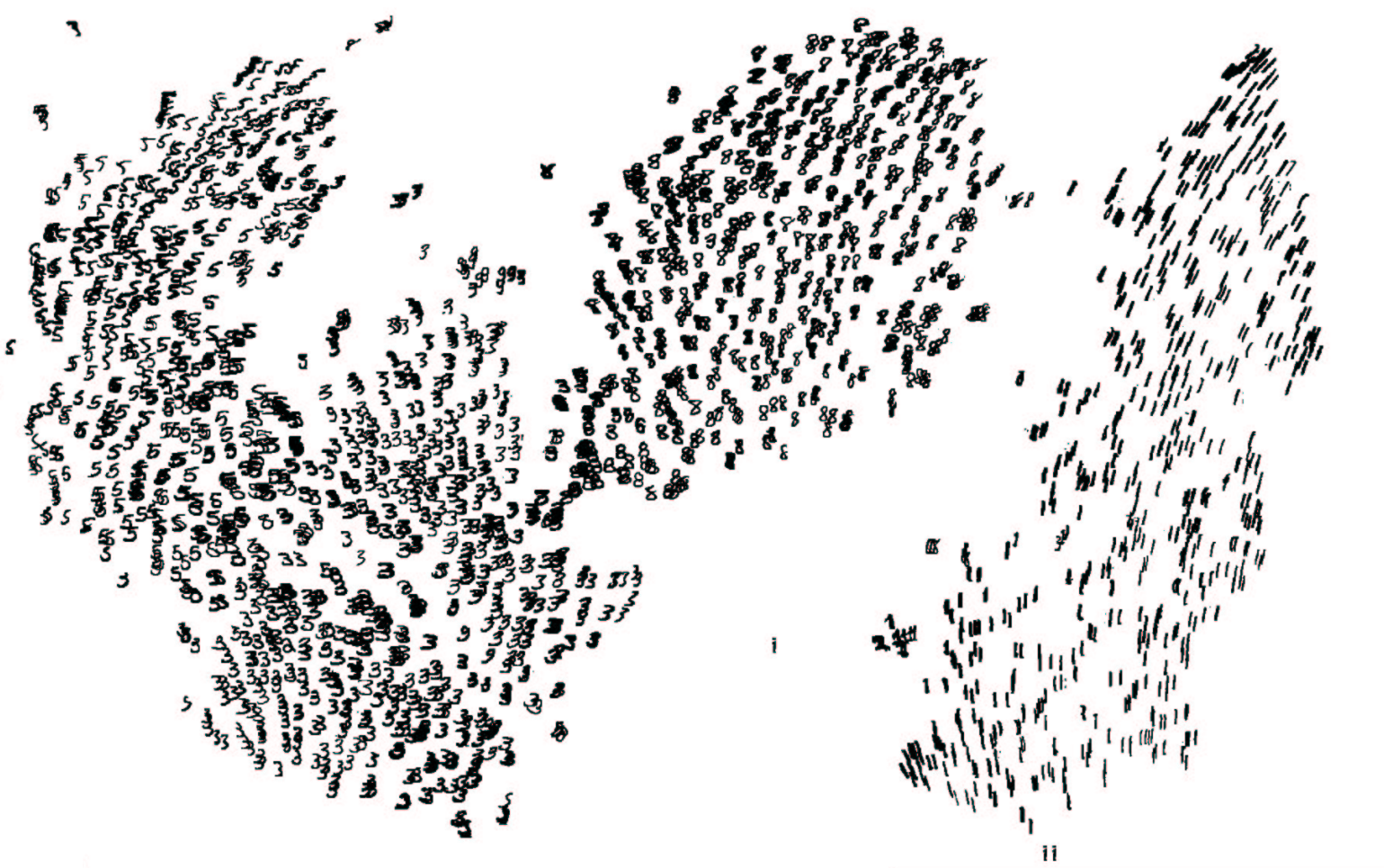
There are also some unusual challenges when doing t-SNE plots. Consider the following t-SNE visualization of word embeddings. Look at the cluster of male names on the left hand side…
A Word Embedding Visualized with t-SNE
(This visualization is deliberately terrible.)
… but you can’t look at the cluster of male names on the left hand side. (It’s frustrating not to be able to hover, isn’t it?) While the points are in the exact same positions as in our earlier visualization, without the ability to look at which words correspond to points, this plot is essentially useless. At best, we can look at it and say that the data probably isn’t random.
The problem is that in dimensionality reduced plots of high-dimensional data, position doesn’t explain the data points. This is true even if you understand precisely what the plot you are looking at is.
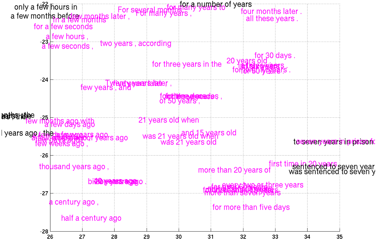
Well, we can fix that. Let’s add back in the tooltip. Now, by hovering over points you can see what word the correspond to. Why don’t you look at the body part cluster?
A Word Embedding Visualized with t-SNE
(This visualization is deliberately terrible, but less than the previous one.)
You are forgiven if you didn’t have the patience to look at several hundred data points in order to find the body part cluster. And, unless you remembered where it was from before, that’s the effort one would expect it to take you.
The ability to inspect points is not sufficient. When dealing with thousands of points, one needs a way to quickly get a high-level view of the data, and then drill in on the parts that are interesting.
This brings us to my personal theory of visualizing high dimensional data (based on my whole three months of working on visualizing it):
- There must be a way to interrogate individual data points.
- There must be a way to get a high-level view of the data.
Interactive visualizations are a really easy way to get both of these properties. But they aren’t the only way. There’s a really beautiful visualization of MNIST in the original t-SNE paper, Maaten & Hinton (2008), on the page labeled 2596:
By directly embedding every MNIST digit’s image in the visualization, Maaten and Hinton made it very easy to inspect individual points. Further, from the ‘texture’ of clusters, one can also quickly recognize their nature.
Unfortunately, that approach only works because MNIST images are small and simple. In their exciting paper on phrase representations, Cho et al. (2014) include some very small subsections of a t-SNE visualization of phrases:
Unfortunately, embedding the phrases directly in the visualization just doesn’t work. They’re too large and clunky. Actually, I just don’t see any good way to visualize this data without using interactive media.
Geometric Fingerprints
Now that we’ve looked at a bunch of exciting representations, let’s return to our simple MNIST networks and examine the representations they form. We’ll use PCA for dimensionality reduction now, since it will allow us to observe some interesting geometric properties of these representations, and because it is less stochastic than the other dimensionality reduction algorithms we’ve discussed.
The following network has a 5 unit sigmoid layer. Such a network would never be used in practice, but is a bit fun to look at.
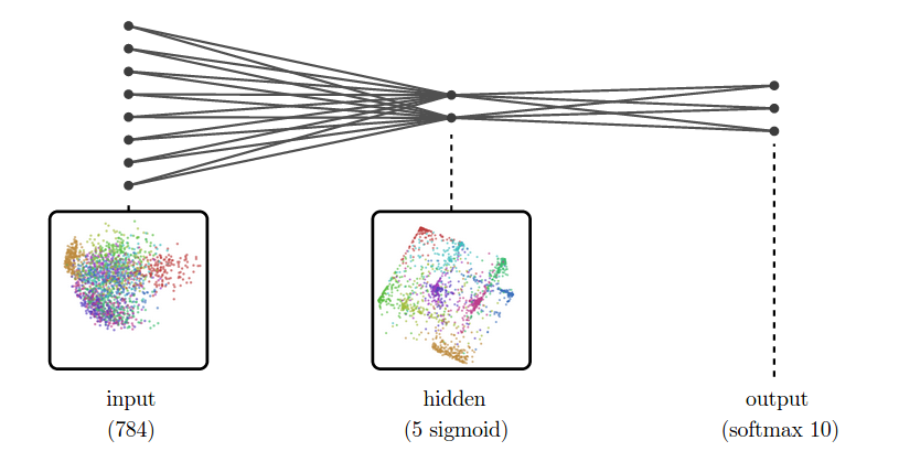
Then network’s hidden representation looks like a projection of a high-dimensional cube. Why? Well, sigmoid units tend to give values close to 0 or 1, and less frequently anything in the middle. If you do that in a bunch of dimensions, you end up with concentration at the corners of a high-dimensional cube and, to a lesser extent, along its edges. PCA then projects this down into two dimensions.
This cube-like structure is a kind of geometric fingerprint of sigmoid layers. Do other activation functions have a similar geometric fingerprint? Let’s look at a ReLU layer.
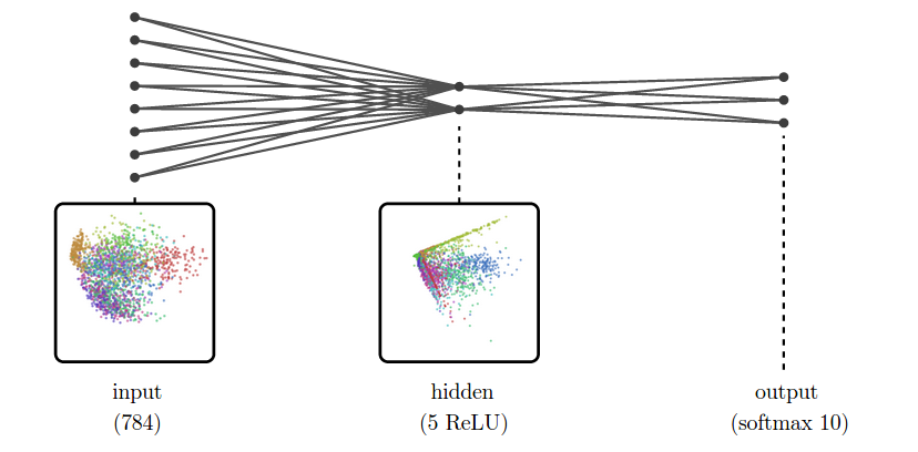
Because ReLU’s have a high probability of being zero, lots of points concentrate on the origin, and along axes. Projected into two dimensions, it looks like a bunch of “spouts” shooting out from the origin.
These geometric properties are much more visible when there are only a few neurons.
The Space of Representations
Every time we train a neural net, we get new representations. This is true even if we train the same network multiple times. The result is that it is very easy to end up with lots of representations of a dataset.
We rarely look at any of these representations, but if we want to, it’s pretty easy to make visualizations of all of them. Here’s a bunch to look at.
The Many Representations of MNIST
Now, while we can visualize a lot of representations like this, it isn’t terribly helpful. What do we learn from it? Not much. We have lots of particular representations, but it’s hard to compare them or get a big picture view.
Let’s focus on comparing representations for a moment. The tricky thing about this is that fundamentally similar neural networks can be very different in ways we don’t care about. Two neurons might be switched. The representation could be rotated or flipped.
Two very similar representations, except for a flip
We want to, somehow, forget about these unimportant differences and focus only on the important differences. We want a canonical form for representations, that encodes only meaningful differences.
Distance seems fundamental, here. All of these unimportant differences are isometries – that is, transformations like rotation or switching two dimensions do not change the distances between points. On the other hand, distance between points is really important: things being close together is a representations way of saying that they are similar, and things being far apart is a representation saying they are different.
Thankfully, there’s an easy way to forget about isometries. For a representation (X), there’s an associated metric function, (d_X), which gives us the distance between pairs of points within that representation. For another representation (Y), (d_X = d_Y) if and only if (X) is isometric to (Y). The metric functions encode precisely the information we want!
We can’t really work with (d_X) because it is actually a function on a very high-dimensional continuous space.4 We need to discretize it for it to be useful.
[D_X = left[begin{array}{cccc}
d_X(x_0, x_0) & d_X(x_1, x_0) & d_X(x_2, x_0) & … \
d_X(x_0, x_1) & d_X(x_1, x_1) & d_X(x_2, x_1) & … \
d_X(x_0, x_2) & d_X(x_1, x_2) & d_X(x_2, x_2) & … \
… & … & … & … \
end{array} right]]
One thing we can do with (D_X) is flatten it to get a vector encoding the properties of the representation (X). We can do this for a lot of representations, and we get a collection of high-dimensional vectors.
The natural thing to do, of course, is to apply dimensionality reduction, such as t-SNE, to our representations. Geoff Hinton dubbed this use of t-SNE “meta-SNE”. But one can also use other kinds of dimensionality reduction.5 6
In the following visualization, there are three boxes. The largest one, on the left, visualizes the space of representations, with every point corresponding to a representation. The points are positioned by dimensionality reduction of the flattened distance matrices, as above. One way to think about this that distance between representations in the visualization represents how much they disagree on which points are similar and which points are different.
Next, the middle box is a regular visualization of a representation of MNIST, like the many we’ve seen previously. It displays which ever representation you hover over in left box. Finally, the right most box displays particular MNIST digits, depending on which point you hover over in the middle box.
The Space of MNIST Representations
Left: Visualization of representations with meta-SNE, points are representations. Middle: Visualization of a particular representation, points are MNIST data points. Right: Image of a particular data point.
This visualization shifts us from looking at trees to seeing the forest. It moves us from looking at representations, to looking at the space of representations. It’s a step up the ladder of abstraction.
Imagine training a neural network and watching its representations wander through this space. You can see how your representations compare to other “landmark” representations from past experiments. If your model’s first layer representation is in the same place a really successful model’s was during training, that’s a good sign! If it’s veering off towards a cluster you know had too high learning rates, you know you should lower it. This can give us qualitative feedback during neural network training.
It also allows us to ask whether two models which achieve comparable results are doing similar things internally or not.
Deep Learning for Visualization
All of the examples above visualize not only the neural network, but the data it operates on. This is because the network is inextricably tied to the data it operates on.7
The visualizations are a bit like looking through a telescope. Just like a telescope transforms the sky into something we can see, the neural network transforms the data into a more accessible form. One learns about the telescope by observing how it magnifies the night sky, but the really remarkable thing is what one learns about the stars. Similarly, visualizing representations teaches us about neural networks, but it teaches us just as much, perhaps more, about the data itself.
(If the telescope is doing a good job, it fades from the consciousness of the person looking through it. But if there’s a scratch on one of the telescope’s lenses, the scratch is highly visible. If one has an example of a better telescope, the flaws in the worse one will suddenly stand out. Similarly, most of what we learn about neural networks from representations is in unexpected behavior, or by comparing representations.)
Understanding data and understanding models that work on that data are intimately linked. In fact, I think that understanding your model has to imply understanding the data it works on. 8
While the idea that we should try to visualize neural networks has existed in our community for a while, this converse idea – that we can use neural networks for visualization – seems equally important is almost entirely unexplored.
Let’s explore it.
Unthinkable Thoughts, Incomprehensible Data
In his talk ‘Media for Thinking the Unthinkable’, Bret Victor raises a really beautiful quote from Richard Hamming:
Just as there are odors that dogs can smell and we cannot, as well as sounds that dogs can hear and we cannot, so too there are wavelengths of light we cannot see and flavors we cannot taste.
Why then, given our brains wired the way they are, does the remark “Perhaps there are thoughts we cannot think,” surprise you?
Evolution, so far, may possibly have blocked us from being able to think in some directions; there could be unthinkable thoughts.
— Richard Hamming, The Unreasonable Effectiveness of Mathematics
Victor continues with his own thoughts:
These sounds that we can’t hear, this light that we can’t see, how do we even know about these things in the first place? Well, we built tools. We built tools that adapt these things that are outside of our senses, to our human bodies, our human senses.
We can’t hear ultrasonic sound, but you hook a microphone up to an oscilloscope and there it is. You’re seeing that sound with your plain old monkey eyes. We can’t see cells and we can’t see galaxies, but we build microscopes and telescopes and these tools adapt the world to our human bodies, to our human senses.
When Hamming says there could be unthinkable thoughts, we have to take that as “Yes, but we build tools that adapt these unthinkable thoughts to the way that our minds work and allow us to think these thoughts that were previously unthinkable.”
— Bret Victor, Media for Thinking the Unthinkable
This quote really resonates with me. As a machine learning researcher, my job is basically to struggle with data that is incomprehensible – literally impossible for the human mind to comprehend – and try to build tools to think about it and work with it.9
However, from the representation perspective, there’s a further natural step to go with this idea…
Representations in Human Vision
Lets consider human vision for a moment. Our ability to see is amazing. The amazing part isn’t our eyes detecting photons, though. That’s the easy, simple part. The amazing thing is the ability of our brain to transform the mess of swirling high-dimensional data into something we can understand. To present it to us so well that it seems simple! We can do this because our brains have highly specialized pathways for processing visual data.
Just as neural networks transform data from the original raw representations into nice representations, the brain transforms our senses from complicated high-dimensional data into nice representations, from the incomprehensible to the comprehensible. My eye detects photons, but before I even become consciously aware of what my eye sees, the data goes through incredibly sophisticated transformations, turning it into something I can reason about.10 The brain does such a good job that vision seems easy! It’s only when you try to understand visual data without using your visual system that you realize how incredibly complicated and difficult to understand it is.
Senses We Don’t Have
Unfortunately, for every sense we have, there are countless others we don’t. Countless modes of experience lost to us. This is a tragedy. Imagine the senses we could have! There are vast collections of text out there: libraries, wikipedia, the Internet as a whole – imagine having a sense that allowed you to see a whole corpus at once, which parts are similar and which are different! Every collision at the Large Hadron Collider is monitored by a battery of different sensors – imagine having a sense that allowed us to ‘see’ collisions as clearly as we can see images! The barrier between us and these potential senses isn’t getting the data, it’s getting the data to our brain in a nice representation.
The easiest way to get new kinds of data into the brain is to simply project it into existing senses. In some very particular cases, this works really well. For example, microscopes and telescopes are extremely good at making a new kind of data accessible by projecting it into our normal visual sense. They work because macroscopic visual data and microscopic visual data are just visual data on different scales, with very similar structure to normal visual data, and are well handled by the same visual processing systems. Much more often, projecting data into an existing sense (for example, with PCA) throws away all but the crudest facets of the data. It’s like taking an image and throwing away everything except the average color. It’s something… but not much.
We can also try to get this data to us symbolically. Of course, rattling off 10,000-dimensional vectors to people is hopeless. But traditional statistics gives us some simple models we can fit, and then discuss using language of means, variance, covariance and so on. Unfortunately, fitting gaussians is like describing clouds as ovals. Talking about the covariance of two variables is like talking about the slope, in a particular direction, of a high-dimensional surface. Even very sophisticated models from statistics seem unable to cope with the complicated, swirling, high-dimensional data we see in problems like vision.
Deep learning gives us models that can work with this data. More that that, it gives us new representations of the data. The representations it produces aren’t optimized to be nice representations for the human brain – I have no idea how one would optimize for that, or even what it would mean – but they are much nicer than the original data. I think that learning representations, with deep learning or other powerful models, is essential to helping humans understand new forms of data.
A Map of Wikipedia
The best example I can give is the visualization of Wikipedia from earlier. Wikipedia is a repository of human knowledge. By combining deep learning and dimensionality reduction, we can make a map of it, as we saw earlier:
Map of Wikipedia
(paragraph vectors and t-SNE – see Example 2 above)
This style of visualization feels important to me. Using deep learning, we’ve made a visualization, an interface, for humans to interact with Wikipedia as a whole. I’m not claiming that it’s a great interface. I’m not even sure I think it is terribly useful. But it’s a starting point and a proof of concept.
Why not just use dimensionality reduction by itself? If we had just used dimensionality reduction, we would be visualizing geometric or topological features of the Wikipedia data. Using deep learning to transform the data allows us to visualize the underlying structure, the important variations – in some cases, the very meaning of the data11 – instead.
I think that high-quality representations have a lot of potential for users interacting with complicated data, going far beyond what is explored here. The most natural direction is machine learning: once you are in a high-quality representation, many normally difficult tasks can be accomplished with very simple techniques and comparatively little data.12 With a curated collection of representations, one could make some really exciting machine learning accessible,13 although it would carry with it challenges for end users14 and the producers of representations.15
Quantifying the Subjective
Reasoning about data through representations can be useful even for kinds of data the human mind understands really well, because it can make explicit and quantifiable things that are normally tacit and subjective.
You probably understand English very well, but much of this knowledge is subjective. The meaning of words is socially constructed, arising from what people mean by them and how they use them. It’s canonicalized in dictionaries, but only to a limited extent. But the subtleties in usage and meaning are very interesting because of how they reflect culture and society. Unfortunately, these things are kind of fuzzy, and one typically needs to rely on anecdotes and personal impressions.
One remarkable property of high-quality word embeddings is that they seem to reify these fuzzy properties into concrete mathematical structures! As mentioned earlier, directions in word embeddings correspond to particular kinds of differences in meaning. For example, there is some direction corresponding to gender. (For more details, see my post Deep Learning, NLP, and Representations.)
By taking the difference of two word vectors, we can get directions for gender. For example, we can get a masculine direction (eg. “man” — “woman”) or a feminine direction (eg. “woman” — “man”). We can also get age directions. For example, we can get an adult direction (eg. “woman” — “girl”) or a child direction (eg. “boy” — “man”).
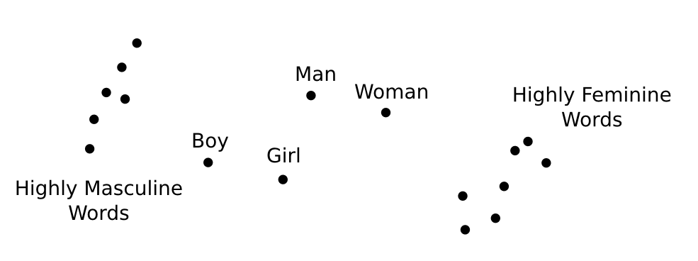
Once we have these directions, there’s a very natural question to ask: which words are furthest in these directions? What are the most masculine or feminine words? The most adult, the most childish? Well, let’s look at the Wikipedia GloVe vectors, from Pennington, et al. at Stanford:
- Masculine words tend to be related to military/extremism (eg. aresenal, tactical, al qaeda), leadership (eg. boss, manager), and sports (eg. game, midfielder).
- Female words tend to be related to reproduction (eg. pregnancy, birth), romance (eg. couples, marriages), healthcare (eg. nurse, patients), and entertainment (eg. actress).
- Adult words tend to be related to power (eg. victory, win), importance (eg. decisive, formidable), politics (eg. political, senate) and tradition (eg. roots, churches).
- Childish words tend to be related to young families (eg. adoption, infant), activities (eg. choir, scouts), items (eg. songs, guitar, comics) and sometimes inheritance (eg. heir, throne).
Of course, these results depend on a lot of details. 16
I’d like to emphasize that which words are feminine or masculine, young or adult, isn’t intrinsic. It’s a reflection of our culture, through our use of language in a cultural artifact. What this might say about our culture is beyond the scope of this essay. My hope is that this trick, and machine learning more broadly, might be a useful tool in sociology, and especially subjects like gender, race, and disability studies.
The Future
Right now machine learning research is mostly about getting computers to be able to understand data that humans do: images, sounds, text, and so on. But the focus is going to shift to getting computers to understand things that humans don’t. We can either figure out how to use this as a bridge to allow humans to understand these things, or we can surrender entire modalities – as rich, perhaps more rich, than vision or sound – to be the sole domain of computers. I think user interface could be the difference between powerful machine learning tools – artificial intelligence – being a black box or a cognitive tool that extends the human mind.
There’s actually two kinds of black boxes we need to avoid. Two slightly different, but closely connected problems. The first problem is that deep learning itself is presently a kind of black box. The second is that tools using deep learning to solve particular problems might be black boxes.
We need to figure out how to open the deep learning black box. One powerful approach is visualizing representations. In this essay, we used interactive media to visualize and explore some powerful models from Google’s deep learning research group. We then observed that particular neural network architectures leave geometric signatures in their representations. Finally, we created the meta-SNE algorithm, in order to step up the ladder of abstraction, and think about the space of neural networks, instead of particular ones.
The problem of particular tools being black boxes is, in some ways, harder, because there’s so much diversity. But a common problem is that humans can’t think about the sort of high-dimensional structures machine learning problems typically involve. We observed that visualizing representations can also be a tool to help humans understand and reason about these structures. We saw that representations can be helpful even for data we understand really well.
These are problems we’re only beginning to attack. I think there’s a lot more for us to uncover here. It’s an odd kind of work, at the intersection of machine learning, mathematics, and user interface. But I think it’s important.
If you enjoyed this post, consider subscribing to my rss feed.
(I would be delighted to hear your comments and thoughts: you can comment inline or at the end. For typos, technical errors, or clarifications you would like to see added, you are encouraged to make a pull request on github.)
Acknowledgements
I’m grateful for the hospitality of Google’s deep learning research group, which had me as an intern while I did most of the work this post is based on. I’m especially grateful to my internship host, Jeff Dean.
I was greatly helped by the comments, advice, and encouragement of many Googlers, both in the deep learning group and outside of it. These include: Greg Corrado, Jon Shlens, Matthieu Devin, Andrew Dai, Quoc Le, Anelia Angelova, Oriol Vinyals, Ilya Sutskever, Ian Goodfellow, Jutta Degener, and Anna Goldie.
I was strongly influenced by the thoughts, comments and notes of Michael Nielsen, especially his notes on Bret Victor’s work. Michael’s thoughts persuaded me that I should think seriously about interactive visualizations for understanding deep learning. The section “Unthinkable Thoughts, Incomprehensible Data” was particularily influenced by him.
I was also helped by the support and comments of a number of other non-Googler friends, including Yoshua Bengio, Laura Ball, Rob Gilson, Henry de Valence, Yomna Nasser, and James Koppel.
This blog post was made possible by a number of wonderful Javascript libraries, including D3.js, MathJax, and jQuery. A big thank you to everyone who contributed to these libraries.
-
The representation perspective is an abstraction over inputs. Instead of trying to understand what the neural network does to a single input, we try to understand what it does to the space of inputs, to the data manifold. It’s a step up the ladder of abstraction. Later, we will take a second step, allowing us to look at the space of neural networks, instead of a single one.↩
-
We categorize words using WordNet synsets. Each synset is labeled something like “region.n.03” (region, noun, meaning 3) or “travel.v.01” (travel, verb, meaning 1).↩
-
It should be noted that, later, Sutskever et al. switched to reversing the order of the input sentence, finding this improved their results.
 ↩
↩ -
The natural way to think about distance between functions is to consider them as infinite dimensional vectors ((f(0), ~ f(1),~ f(2)…)). In the case of a function on the real numbers or on (mathbb{R}^n), it’s a (2^{aleph_0}) dimensional vector! While we can actually represent the function finitely (because we know it’s based on a neural network, which has a finite number of paramaters) it’s really hard to actually calculate distances.↩
-
I’ve heard that some similar techniques may be used in neuroscience, where one often needs to compare different representations of the same data. Further, in a previous post, John MacCuish commented that one could use the Mantel Test on the distance matrices to compare representations – this gets at a very similar idea!↩
-
There are some variations you can do on the basic meta-SNE algorithm. For example, meta-SNE analyzes how much representations agree on which data points are similar, by comparing distance between the points in different representations. But we can also compare how much representations agree on analogies, on the manner in which things are different, by comparing the distance between differences of vectors in different representations. In principle, this information is encoded in the distances between data points, but one can make it much more explicit. It may also be the case that we care more about which networks are very similar, in which case we could apply some non-linearity pointwise to the distance matrix, to exaggerate the difference between close and not-close data points.↩
-
The neural network is a function with the domain of the data manifold it was trained on.↩
-
People sometimes complain: “Neural networks are so hard to understand! Why can’t we use understandable models, like SVMs?” Well, you understand SVMs, and you don’t understand visual pattern recognition. If SVMs could solve visual pattern recognition, you would understand it. Therefore, SVMs are not capable of this, nor is any other model you can really understand. (I don’t mean this to be a ‘proof’ obviously, but I am pretty serious about this view.)↩
-
You could imagine defining a field this way, as attempting to build tools for thinking about and working with the complicated high-dimensional probability distributions we see in the real world. The field you get isn’t quite machine learning, but it has a lot of overlap. It actually feels more compelling to me. Perhaps this is “data science”?↩
-
As someone without a neuroscience background, I feel a bit nervous making remarks like this. That said, I think what I’m mostly saying is an interpretation, an abstraction, over some fairly basic facts about how human vision works. I also know that at least some neuroscientists subscribe to this interpretation and seriously look at things through this sort of lens. For example, see DiCarlo and Cox’s paper ‘Untangling invariant object recognition’.↩
-
This is a very bold claim. My defense is this: word embedding models seem to encode semantic meaning in directions, creating a “semantic vector space.” Paragraph vectors (at least the kind that we’re using) do the same. Somehow, these models seem to discover human meaning while learning the structure of the space. The results of the DeViSE paper suggest that this may be somewhat general in good high-level representations.↩
-
This is some combination of transfer learning, pretraining, and multi-task learning. How well it works varies, but there’s certainly a lot of successes. Obviously, the ideal is to have a lot of data to train a representation specifically for your task. But failing that, we can also try to make very transferable representations, possibly by training them for a bunch of different tasks.↩
-
Curating large collections of structured data has lead to some really interesting tools (for example, Wolfram Alpha). My intuition is that curating a collection of high-quality representations for different kinds of data could also be really interesting. I think MetaMind is the closest thing I know of to this, right now.↩
-
It seems like a lot of the problems that exist with proprietary file formats could end up happening here. An end user could very easily end up tied to a particular representation. Do we need open or standardized representations?↩
-
The problem with just releasing representations, from the perspective of the model producer, is what Geoff Hinton calls “Dark Knowledge”. Representations subtly encode a lot of the knowledge of your model. By releasing representations, organizations are implicitly releasing a significant amount of information about their model.↩
-
The answer depends a lot on the corpus you train on. If you train your word embedding on a news corpus, that will be different than if you train it on Wikipedia. And I assume if you trained on a corpus of 19th century literature, that would be very different again. It also depends on your model, and how well you trained it. The precise interpretation is obviously sensitive to the model. But, generally, it will be something like this: There is a certain difference in how language is used around the word “man” and the word “woman”; which words cause language around them to change most in that manner? (Replace “man” and “woman” for whatever you want.)↩
Presentation on theme: «Bag of Visual Words for Image Representation & Visual Search Jianping Fan Dept of Computer Science UNC-Charlotte.»— Presentation transcript:
1
Bag of Visual Words for Image Representation & Visual Search Jianping Fan Dept of Computer Science UNC-Charlotte
2
1. Interest Point Extraction & SIFT 2. Clustering for Dictionary Learning 3. Bag of Visual Words 4. Image Representation & Applications Bag-of-Visual-Words
3
Interest Point Extraction Scale-space extrema detection –Uses difference-of-Gaussian function Keypoint localization –Sub-pixel location and scale fit to a model Orientation assignment –1 or more for each keypoint Keypoint descriptor –Created from local image gradients
4
Scale space Definition: where Interest Point Extraction
5
Scale space Keypoints are detected using scale-space extrema in difference-of-Gaussian function D D definition: Efficient to compute
6
Relationship of D to Close approximation to scale-normalized Laplacian of Gaussian, Diffusion equation: Approximate ∂G/∂σ: –giving, When D has scales differing by a constant factor it already incorporates the σ 2 scale normalization required for scale-invariance
7
Interest Point Extraction
8
Difference-of-Gaussian images … first octave … … second octave … … third octave … fourth octave … …
9
Finding extrema Sample point is selected only if it is a minimum or a maximum of these points DoG scale space Extrema in this image
10
Localization 3D quadratic function is fit to the local sample points Start with Taylor expansion with sample point as the origin –where Take the derivative with respect to X, and set it to 0, giving is the location of the keypoint This is a 3×3 linear system
11
Localization Derivatives approximated by finite differences, –example: If X is > 0.5 in any dimension, process repeated
12
Filtering Contrast (use prev. equation): –If | D(X) | < 0.03, throw it out Edge-iness: –Use ratio of principal curvatures to throw out poorly defined peaks –Curvatures come from Hessian: –Ratio of Trace(H) 2 and Determinant(H) –If ratio > (r+1) 2 /(r), throw it out (SIFT uses r=10)
13
Orientation assignment Descriptor computed relative to keypoint’s orientation achieves rotation invariance Precomputed along with mag. for all levels (useful in descriptor computation) Multiple orientations assigned to keypoints from an orientation histogram –Significantly improve stability of matching
14
Keypoint images
15
Descriptor Descriptor has 3 dimensions (x,y,θ) Orientation histogram of gradient magnitudes Position and orientation of each gradient sample rotated relative to keypoint orientation
16
Descriptor Best results achieved with 4x4x8 = 128 descriptor size Normalize to unit length –Reduces effect of illumination change Cap each element to 0.2, normalize again –Reduces non-linear illumination changes –0.2 determined experimentally
17
PCA-SIFT Different descriptor (same keypoints) Apply PCA to the gradient patch Descriptor size is 20 (instead of 128) More robust, faster
18
Interest Points & SIFT Features
19
Summary Scale space Difference-of-Gaussian Localization Filtering Orientation assignment Descriptor, 128 elements
20
Dictionary Learning
21
22
23
24
25
26
27
Quantization for Identification
28
28 Sparse Coding & Dictionary Learning Dictionary learning and sparse coding Sparse factor analysis model (Factor/feature/dish/dictionary atom) Indian Buffet process and beta process
29
Dictionary Learning
30
31
32
33
34
Image Representation via Bag-of-Visual-Words Dictionary
35
36
37
38
39
40
Application for Visual Search
41
How to do database indexing?
42
Application for Visual Search Visual Phrases & Contexts?
43
Multi-Resolution SIFT
44
45
46
47
48
49
50
51
52
53
54
55
56
57
58
59
60
61
62
Become a DeepAI PRO


500 generated images per month
Private image generation
Complete styles library
API access
Ad-free experience
AI Chat access with Genius Mode
*
This is a recurring payment that will happen monthly
*
If you exceed more than 500 images, they will be charged at a rate of $5 per 500 images
Pay as you go
Private image generation
Complete styles library
API access
Ad-free experience