
14 May 2019
In this post, I take an in-depth look at word embeddings produced by Google’s BERT and show you how to get started with BERT by producing your own word embeddings.
This post is presented in two forms–as a blog post here and as a Colab notebook here.
The content is identical in both, but:
- The blog post format may be easier to read, and includes a comments section for discussion.
- The Colab Notebook will allow you to run the code and inspect it as you read through.
Update 5/27/20 — I’ve updated this post to use the new transformers library from huggingface in place of the old pytorch-pretrained-bert library. You can still find the old post / Notebook here if you need it.
By Chris McCormick and Nick Ryan
Contents
- Contents
- Introduction
- History
- What is BERT?
- Why BERT embeddings?
- 1. Loading Pre-Trained BERT
- 2. Input Formatting
- 2.1. Special Tokens
- 2.2. Tokenization
- 2.3. Segment ID
- 3. Extracting Embeddings
- 3.1. Running BERT on our text
- 3.2. Understanding the Output
- 3.3. Creating word and sentence vectors from hidden states
- Word Vectors
- Sentence Vectors
- 3.4. Confirming contextually dependent vectors
- 3.5. Pooling Strategy & Layer Choice
- 4. Appendix
- 4.1. Special tokens
- 4.2. Out of vocabulary words
- 4.3. Similarity metrics
- 4.4. Implementations
- Cite
Introduction
History
2018 was a breakthrough year in NLP. Transfer learning, particularly models like Allen AI’s ELMO, OpenAI’s Open-GPT, and Google’s BERT allowed researchers to smash multiple benchmarks with minimal task-specific fine-tuning and provided the rest of the NLP community with pretrained models that could easily (with less data and less compute time) be fine-tuned and implemented to produce state of the art results. Unfortunately, for many starting out in NLP and even for some experienced practicioners, the theory and practical application of these powerful models is still not well understood.
What is BERT?
BERT (Bidirectional Encoder Representations from Transformers), released in late 2018, is the model we will use in this tutorial to provide readers with a better understanding of and practical guidance for using transfer learning models in NLP. BERT is a method of pretraining language representations that was used to create models that NLP practicioners can then download and use for free. You can either use these models to extract high quality language features from your text data, or you can fine-tune these models on a specific task (classification, entity recognition, question answering, etc.) with your own data to produce state of the art predictions.
Why BERT embeddings?
In this tutorial, we will use BERT to extract features, namely word and sentence embedding vectors, from text data. What can we do with these word and sentence embedding vectors? First, these embeddings are useful for keyword/search expansion, semantic search and information retrieval. For example, if you want to match customer questions or searches against already answered questions or well documented searches, these representations will help you accuratley retrieve results matching the customer’s intent and contextual meaning, even if there’s no keyword or phrase overlap.
Second, and perhaps more importantly, these vectors are used as high-quality feature inputs to downstream models. NLP models such as LSTMs or CNNs require inputs in the form of numerical vectors, and this typically means translating features like the vocabulary and parts of speech into numerical representations. In the past, words have been represented either as uniquely indexed values (one-hot encoding), or more helpfully as neural word embeddings where vocabulary words are matched against the fixed-length feature embeddings that result from models like Word2Vec or Fasttext. BERT offers an advantage over models like Word2Vec, because while each word has a fixed representation under Word2Vec regardless of the context within which the word appears, BERT produces word representations that are dynamically informed by the words around them. For example, given two sentences:
“The man was accused of robbing a bank.”
“The man went fishing by the bank of the river.”
Word2Vec would produce the same word embedding for the word “bank” in both sentences, while under BERT the word embedding for “bank” would be different for each sentence. Aside from capturing obvious differences like polysemy, the context-informed word embeddings capture other forms of information that result in more accurate feature representations, which in turn results in better model performance.
From an educational standpoint, a close examination of BERT word embeddings is a good way to get your feet wet with BERT and its family of transfer learning models, and sets us up with some practical knowledge and context to better understand the inner details of the model in later tutorials.
Onward!

1. Loading Pre-Trained BERT
Install the pytorch interface for BERT by Hugging Face. (This library contains interfaces for other pretrained language models like OpenAI’s GPT and GPT-2.)
We’ve selected the pytorch interface because it strikes a nice balance between the high-level APIs (which are easy to use but don’t provide insight into how things work) and tensorflow code (which contains lots of details but often sidetracks us into lessons about tensorflow, when the purpose here is BERT!).
If you’re running this code on Google Colab, you will have to install this library each time you reconnect; the following cell will take care of that for you.
!pip install transformers
Now let’s import pytorch, the pretrained BERT model, and a BERT tokenizer.
We’ll explain the BERT model in detail in a later tutorial, but this is the pre-trained model released by Google that ran for many, many hours on Wikipedia and Book Corpus, a dataset containing +10,000 books of different genres. This model is responsible (with a little modification) for beating NLP benchmarks across a range of tasks. Google released a few variations of BERT models, but the one we’ll use here is the smaller of the two available sizes (“base” and “large”) and ignores casing, hence “uncased.””
transformers provides a number of classes for applying BERT to different tasks (token classification, text classification, …). Here, we’re using the basic BertModel which has no specific output task–it’s a good choice for using BERT just to extract embeddings.
import torch
from transformers import BertTokenizer, BertModel

# OPTIONAL: if you want to have more information on what's happening, activate the logger as follows
import logging
#logging.basicConfig(level=logging.INFO)

import matplotlib.pyplot as plt
% matplotlib inline

# Load pre-trained model tokenizer (vocabulary)
tokenizer = BertTokenizer.from_pretrained('bert-base-uncased')
2. Input Formatting
Because BERT is a pretrained model that expects input data in a specific format, we will need:
- A special token,
[SEP], to mark the end of a sentence, or the separation between two sentences - A special token,
[CLS], at the beginning of our text. This token is used for classification tasks, but BERT expects it no matter what your application is. - Tokens that conform with the fixed vocabulary used in BERT
- The Token IDs for the tokens, from BERT’s tokenizer
- Mask IDs to indicate which elements in the sequence are tokens and which are padding elements
- Segment IDs used to distinguish different sentences
- Positional Embeddings used to show token position within the sequence
Luckily, the transformers interface takes care of all of the above requirements (using the tokenizer.encode_plus function).
Since this is intended as an introduction to working with BERT, though, we’re going to perform these steps in a (mostly) manual way.
For an example of using
tokenizer.encode_plus, see the next post on Sentence Classification here.
2.1. Special Tokens
BERT can take as input either one or two sentences, and uses the special token [SEP] to differentiate them. The [CLS] token always appears at the start of the text, and is specific to classification tasks.
Both tokens are always required, however, even if we only have one sentence, and even if we are not using BERT for classification. That’s how BERT was pre-trained, and so that’s what BERT expects to see.
2 Sentence Input:
[CLS] The man went to the store. [SEP] He bought a gallon of milk.
1 Sentence Input:
[CLS] The man went to the store. [SEP]
2.2. Tokenization
BERT provides its own tokenizer, which we imported above. Let’s see how it handles the below sentence.
text = "Here is the sentence I want embeddings for."
marked_text = "[CLS] " + text + " [SEP]"

# Tokenize our sentence with the BERT tokenizer.
tokenized_text = tokenizer.tokenize(marked_text)

# Print out the tokens.
print (tokenized_text)
['[CLS]', 'here', 'is', 'the', 'sentence', 'i', 'want', 'em', '##bed', '##ding', '##s', 'for', '.', '[SEP]']
Notice how the word “embeddings” is represented:
['em', '##bed', '##ding', '##s']
The original word has been split into smaller subwords and characters. The two hash signs preceding some of these subwords are just our tokenizer’s way to denote that this subword or character is part of a larger word and preceded by another subword. So, for example, the ‘##bed’ token is separate from the ‘bed’ token; the first is used whenever the subword ‘bed’ occurs within a larger word and the second is used explicitly for when the standalone token ‘thing you sleep on’ occurs.
Why does it look this way? This is because the BERT tokenizer was created with a WordPiece model. This model greedily creates a fixed-size vocabulary of individual characters, subwords, and words that best fits our language data. Since the vocabulary limit size of our BERT tokenizer model is 30,000, the WordPiece model generated a vocabulary that contains all English characters plus the ~30,000 most common words and subwords found in the English language corpus the model is trained on. This vocabulary contains four things:
- Whole words
- Subwords occuring at the front of a word or in isolation (“em” as in “embeddings” is assigned the same vector as the standalone sequence of characters “em” as in “go get em” )
- Subwords not at the front of a word, which are preceded by ‘##’ to denote this case
- Individual characters
To tokenize a word under this model, the tokenizer first checks if the whole word is in the vocabulary. If not, it tries to break the word into the largest possible subwords contained in the vocabulary, and as a last resort will decompose the word into individual characters. Note that because of this, we can always represent a word as, at the very least, the collection of its individual characters.
As a result, rather than assigning out of vocabulary words to a catch-all token like ‘OOV’ or ‘UNK,’ words that are not in the vocabulary are decomposed into subword and character tokens that we can then generate embeddings for.
So, rather than assigning “embeddings” and every other out of vocabulary word to an overloaded unknown vocabulary token, we split it into subword tokens [‘em’, ‘##bed’, ‘##ding’, ‘##s’] that will retain some of the contextual meaning of the original word. We can even average these subword embedding vectors to generate an approximate vector for the original word.
(For more information about WordPiece, see the original paper and further disucssion in Google’s Neural Machine Translation System.)
Here are some examples of the tokens contained in our vocabulary. Tokens beginning with two hashes are subwords or individual characters.
For an exploration of the contents of BERT’s vocabulary, see this notebook I created and the accompanying YouTube video here.
list(tokenizer.vocab.keys())[5000:5020]
['knight',
 'lap',
 'survey',
 'ma',
 '##ow',
 'noise',
 'billy',
 '##ium',
 'shooting',
 'guide',
 'bedroom',
 'priest',
 'resistance',
 'motor',
 'homes',
 'sounded',
 'giant',
 '##mer',
 '150',
 'scenes']
After breaking the text into tokens, we then have to convert the sentence from a list of strings to a list of vocabulary indeces.
From here on, we’ll use the below example sentence, which contains two instances of the word “bank” with different meanings.
# Define a new example sentence with multiple meanings of the word "bank"
text = "After stealing money from the bank vault, the bank robber was seen "
       "fishing on the Mississippi river bank."

# Add the special tokens.
marked_text = "[CLS] " + text + " [SEP]"

# Split the sentence into tokens.
tokenized_text = tokenizer.tokenize(marked_text)

# Map the token strings to their vocabulary indeces.
indexed_tokens = tokenizer.convert_tokens_to_ids(tokenized_text)

# Display the words with their indeces.
for tup in zip(tokenized_text, indexed_tokens):
    print('{:<12} {:>6,}'.format(tup[0], tup[1]))
[CLS]           101
after         2,044
stealing     11,065
money         2,769
from          2,013
the           1,996
bank          2,924
vault        11,632
,             1,010
the           1,996
bank          2,924
robber       27,307
was           2,001
seen          2,464
fishing       5,645
on            2,006
the           1,996
mississippi   5,900
river         2,314
bank          2,924
.             1,012
[SEP]           102
2.3. Segment ID
BERT is trained on and expects sentence pairs, using 1s and 0s to distinguish between the two sentences. That is, for each token in “tokenized_text,” we must specify which sentence it belongs to: sentence 0 (a series of 0s) or sentence 1 (a series of 1s). For our purposes, single-sentence inputs only require a series of 1s, so we will create a vector of 1s for each token in our input sentence.
If you want to process two sentences, assign each word in the first sentence plus the ‘[SEP]’ token a 0, and all tokens of the second sentence a 1.
# Mark each of the 22 tokens as belonging to sentence "1".
segments_ids = [1] * len(tokenized_text)

print (segments_ids)
[1, 1, 1, 1, 1, 1, 1, 1, 1, 1, 1, 1, 1, 1, 1, 1, 1, 1, 1, 1, 1, 1]
3.1. Running BERT on our text
Next we need to convert our data to torch tensors and call the BERT model. The BERT PyTorch interface requires that the data be in torch tensors rather than Python lists, so we convert the lists here — this does not change the shape or the data.
# Convert inputs to PyTorch tensors
tokens_tensor = torch.tensor([indexed_tokens])
segments_tensors = torch.tensor([segments_ids])
Calling from_pretrained will fetch the model from the internet. When we load the bert-base-uncased, we see the definition of the model printed in the logging. The model is a deep neural network with 12 layers! Explaining the layers and their functions is outside the scope of this post, and you can skip over this output for now.
model.eval() puts our model in evaluation mode as opposed to training mode. In this case, evaluation mode turns off dropout regularization which is used in training.
# Load pre-trained model (weights)
model = BertModel.from_pretrained('bert-base-uncased',
                                  output_hidden_states = True, # Whether the model returns all hidden-states.
                                  )

# Put the model in "evaluation" mode, meaning feed-forward operation.
model.eval()
Note: I’ve removed the output from the blog post since it is so lengthy. You can find it in the Colab Notebook here if you are interested.
Next, let’s evaluate BERT on our example text, and fetch the hidden states of the network!
Side note: torch.no_grad tells PyTorch not to construct the compute graph during this forward pass (since we won’t be running backprop here)–this just reduces memory consumption and speeds things up a little.
# Run the text through BERT, and collect all of the hidden states produced
# from all 12 layers.
with torch.no_grad():

    outputs = model(tokens_tensor, segments_tensors)

    # Evaluating the model will return a different number of objects based on
    # how it's  configured in the `from_pretrained` call earlier. In this case,
    # becase we set `output_hidden_states = True`, the third item will be the
    # hidden states from all layers. See the documentation for more details:
    # https://huggingface.co/transformers/model_doc/bert.html#bertmodel
    hidden_states = outputs[2]
3.2. Understanding the Output
The full set of hidden states for this model, stored in the object hidden_states, is a little dizzying. This object has four dimensions, in the following order:
- The layer number (13 layers)
- The batch number (1 sentence)
- The word / token number (22 tokens in our sentence)
- The hidden unit / feature number (768 features)
Wait, 13 layers? Doesn’t BERT only have 12? It’s 13 because the first element is the input embeddings, the rest is the outputs of each of BERT’s 12 layers.
That’s 219,648 unique values just to represent our one sentence!
The second dimension, the batch size, is used when submitting multiple sentences to the model at once; here, though, we just have one example sentence.
print ("Number of layers:", len(hidden_states), "  (initial embeddings + 12 BERT layers)")
layer_i = 0

print ("Number of batches:", len(hidden_states[layer_i]))
batch_i = 0

print ("Number of tokens:", len(hidden_states[layer_i][batch_i]))
token_i = 0

print ("Number of hidden units:", len(hidden_states[layer_i][batch_i][token_i]))
Number of layers: 13   (initial embeddings + 12 BERT layers)
Number of batches: 1
Number of tokens: 22
Number of hidden units: 768
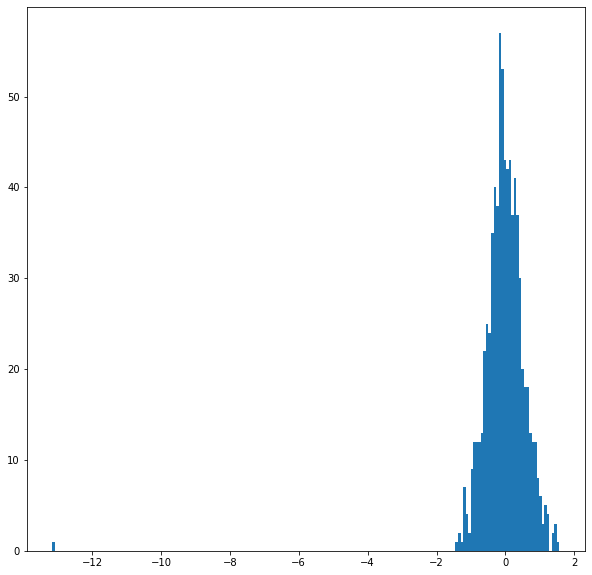
Let’s take a quick look at the range of values for a given layer and token.
You’ll find that the range is fairly similar for all layers and tokens, with the majority of values falling between [-2, 2], and a small smattering of values around -10.
# For the 5th token in our sentence, select its feature values from layer 5.
token_i = 5
layer_i = 5
vec = hidden_states[layer_i][batch_i][token_i]

# Plot the values as a histogram to show their distribution.
plt.figure(figsize=(10,10))
plt.hist(vec, bins=200)
plt.show()
Grouping the values by layer makes sense for the model, but for our purposes we want it grouped by token.
Current dimensions:
[# layers, # batches, # tokens, # features]
Desired dimensions:
[# tokens, # layers, # features]
Luckily, PyTorch includes the permute function for easily rearranging the dimensions of a tensor.
However, the first dimension is currently a Python list!
# `hidden_states` is a Python list.
print('      Type of hidden_states: ', type(hidden_states))

# Each layer in the list is a torch tensor.
print('Tensor shape for each layer: ', hidden_states[0].size())
      Type of hidden_states:  <class 'tuple'>
Tensor shape for each layer:  torch.Size([1, 22, 768])
Let’s combine the layers to make this one whole big tensor.
# Concatenate the tensors for all layers. We use `stack` here to
# create a new dimension in the tensor.
token_embeddings = torch.stack(hidden_states, dim=0)

token_embeddings.size()
torch.Size([13, 1, 22, 768])
Let’s get rid of the “batches” dimension since we don’t need it.
# Remove dimension 1, the "batches".
token_embeddings = torch.squeeze(token_embeddings, dim=1)

token_embeddings.size()
torch.Size([13, 22, 768])
Finally, we can switch around the “layers” and “tokens” dimensions with permute.
# Swap dimensions 0 and 1.
token_embeddings = token_embeddings.permute(1,0,2)

token_embeddings.size()
torch.Size([22, 13, 768])
Now, what do we do with these hidden states? We would like to get individual vectors for each of our tokens, or perhaps a single vector representation of the whole sentence, but for each token of our input we have 13 separate vectors each of length 768.
In order to get the individual vectors we will need to combine some of the layer vectors…but which layer or combination of layers provides the best representation?
Unfortunately, there’s no single easy answer… Let’s try a couple reasonable approaches, though. Afterwards, I’ll point you to some helpful resources which look into this question further.
Word Vectors
To give you some examples, let’s create word vectors two ways.
First, let’s concatenate the last four layers, giving us a single word vector per token. Each vector will have length 4 x 768 = 3,072.
# Stores the token vectors, with shape [22 x 3,072]
token_vecs_cat = []

# `token_embeddings` is a [22 x 12 x 768] tensor.

# For each token in the sentence...
for token in token_embeddings:

    # `token` is a [12 x 768] tensor

    # Concatenate the vectors (that is, append them together) from the last
    # four layers.
    # Each layer vector is 768 values, so `cat_vec` is length 3,072.
    cat_vec = torch.cat((token[-1], token[-2], token[-3], token[-4]), dim=0)

    # Use `cat_vec` to represent `token`.
    token_vecs_cat.append(cat_vec)

print ('Shape is: %d x %d' % (len(token_vecs_cat), len(token_vecs_cat[0])))
As an alternative method, let’s try creating the word vectors by summing together the last four layers.
# Stores the token vectors, with shape [22 x 768]
token_vecs_sum = []

# `token_embeddings` is a [22 x 12 x 768] tensor.

# For each token in the sentence...
for token in token_embeddings:

    # `token` is a [12 x 768] tensor

    # Sum the vectors from the last four layers.
    sum_vec = torch.sum(token[-4:], dim=0)

    # Use `sum_vec` to represent `token`.
    token_vecs_sum.append(sum_vec)

print ('Shape is: %d x %d' % (len(token_vecs_sum), len(token_vecs_sum[0])))
Sentence Vectors
To get a single vector for our entire sentence we have multiple application-dependent strategies, but a simple approach is to average the second to last hiden layer of each token producing a single 768 length vector.
# `hidden_states` has shape [13 x 1 x 22 x 768]

# `token_vecs` is a tensor with shape [22 x 768]
token_vecs = hidden_states[-2][0]

# Calculate the average of all 22 token vectors.
sentence_embedding = torch.mean(token_vecs, dim=0)
print ("Our final sentence embedding vector of shape:", sentence_embedding.size())
Our final sentence embedding vector of shape: torch.Size([768])
3.4. Confirming contextually dependent vectors
To confirm that the value of these vectors are in fact contextually dependent, let’s look at the different instances of the word “bank” in our example sentence:
“After stealing money from the bank vault, the bank robber was seen fishing on the Mississippi river bank.”
Let’s find the index of those three instances of the word “bank” in the example sentence.
for i, token_str in enumerate(tokenized_text):
  print (i, token_str)
0 [CLS]
1 after
2 stealing
3 money
4 from
5 the
6 bank
7 vault
8 ,
9 the
10 bank
11 robber
12 was
13 seen
14 fishing
15 on
16 the
17 mississippi
18 river
19 bank
20 .
21 [SEP]
They are at 6, 10, and 19.
For this analysis, we’ll use the word vectors that we created by summing the last four layers.
We can try printing out their vectors to compare them.
print('First 5 vector values for each instance of "bank".')
print('')
print("bank vault   ", str(token_vecs_sum[6][:5]))
print("bank robber  ", str(token_vecs_sum[10][:5]))
print("river bank   ", str(token_vecs_sum[19][:5]))
First 5 vector values for each instance of "bank".

bank vault    tensor([ 3.3596, -2.9805, -1.5421,  0.7065,  2.0031])
bank robber   tensor([ 2.7359, -2.5577, -1.3094,  0.6797,  1.6633])
river bank    tensor([ 1.5266, -0.8895, -0.5152, -0.9298,  2.8334])
We can see that the values differ, but let’s calculate the cosine similarity between the vectors to make a more precise comparison.
from scipy.spatial.distance import cosine

# Calculate the cosine similarity between the word bank
# in "bank robber" vs "river bank" (different meanings).
diff_bank = 1 - cosine(token_vecs_sum[10], token_vecs_sum[19])

# Calculate the cosine similarity between the word bank
# in "bank robber" vs "bank vault" (same meaning).
same_bank = 1 - cosine(token_vecs_sum[10], token_vecs_sum[6])

print('Vector similarity for  *similar*  meanings:  %.2f' % same_bank)
print('Vector similarity for *different* meanings:  %.2f' % diff_bank)
Vector similarity for  *similar*  meanings:  0.94
Vector similarity for *different* meanings:  0.69
This looks pretty good!
3.5. Pooling Strategy & Layer Choice
Below are a couple additional resources for exploring this topic.
BERT Authors
The BERT authors tested word-embedding strategies by feeding different vector combinations as input features to a BiLSTM used on a named entity recognition task and observing the resulting F1 scores.
(Image from Jay Allamar’s blog)
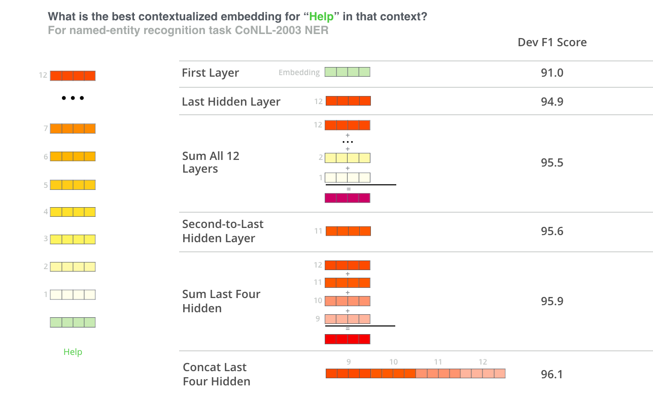
While concatenation of the last four layers produced the best results on this specific task, many of the other methods come in a close second and in general it is advisable to test different versions for your specific application: results may vary.
This is partially demonstrated by noting that the different layers of BERT encode very different kinds of information, so the appropriate pooling strategy will change depending on the application because different layers encode different kinds of information.
Han Xiao’s BERT-as-service
Han Xiao created an open-source project named bert-as-service on GitHub which is intended to create word embeddings for your text using BERT. Han experimented with different approaches to combining these embeddings, and shared some conclusions and rationale on the FAQ page of the project.
bert-as-service, by default, uses the outputs from the second-to-last layer of the model.
I would summarize Han’s perspective by the following:
- The embeddings start out in the first layer as having no contextual information (i.e., the meaning of the initial ‘bank’ embedding isn’t specific to river bank or financial bank).
- As the embeddings move deeper into the network, they pick up more and more contextual information with each layer.
- As you approach the final layer, however, you start picking up information that is specific to BERT’s pre-training tasks (the “Masked Language Model” (MLM) and “Next Sentence Prediction” (NSP)).
- What we want is embeddings that encode the word meaning well…
- BERT is motivated to do this, but it is also motivated to encode anything else that would help it determine what a missing word is (MLM), or whether the second sentence came after the first (NSP).
- The second-to-last layer is what Han settled on as a reasonable sweet-spot.
4. Appendix
4.1. Special tokens
It should be noted that although the [CLS] acts as an “aggregate representation” for classification tasks, this is not the best choice for a high quality sentence embedding vector. According to BERT author Jacob Devlin: “I’m not sure what these vectors are, since BERT does not generate meaningful sentence vectors. It seems that this is is doing average pooling over the word tokens to get a sentence vector, but we never suggested that this will generate meaningful sentence representations.”
(However, the [CLS] token does become meaningful if the model has been fine-tuned, where the last hidden layer of this token is used as the “sentence vector” for sequence classification.)
4.2. Out of vocabulary words
For out of vocabulary words that are composed of multiple sentence and character-level embeddings, there is a further issue of how best to recover this embedding. Averaging the embeddings is the most straightforward solution (one that is relied upon in similar embedding models with subword vocabularies like fasttext), but summation of subword embeddings and simply taking the last token embedding (remember that the vectors are context sensitive) are acceptable alternative strategies.
4.3. Similarity metrics
It is worth noting that word-level similarity comparisons are not appropriate with BERT embeddings because these embeddings are contextually dependent, meaning that the word vector changes depending on the sentence it appears in. This allows wonderful things like polysemy so that e.g. your representation encodes river “bank” and not a financial institution “bank”, but makes direct word-to-word similarity comparisons less valuable. However, for sentence embeddings similarity comparison is still valid such that one can query, for example, a single sentence against a dataset of other sentences in order to find the most similar. Depending on the similarity metric used, the resulting similarity values will be less informative than the relative ranking of similarity outputs since many similarity metrics make assumptions about the vector space (equally-weighted dimensions, for example) that do not hold for our 768-dimensional vector space.
4.4. Implementations
You can use the code in this notebook as the foundation of your own application to extract BERT features from text. However, official tensorflow and well-regarded pytorch implementations already exist that do this for you. Additionally, bert-as-a-service is an excellent tool designed specifically for running this task with high performance, and is the one I would recommend for production applications. The author has taken great care in the tool’s implementation and provides excellent documentation (some of which was used to help create this tutorial) to help users understand the more nuanced details the user faces, like resource management and pooling strategy.
Cite
Chris McCormick and Nick Ryan. (2019, May 14). BERT Word Embeddings Tutorial. Retrieved from http://www.mccormickml.com
@engrsfi
import tensorflow as tf
from transformers import BertTokenizer, TFBertModeltokenizer = BertTokenizer.from_pretrained(‘bert-base-uncased’)
model = TFBertModel.from_pretrained(‘bert-base-uncased’)
input_ids = tf.constant(tokenizer.encode(«Hello, my dog is cute»))[None, :] # Batch size 1
outputs = model(input_ids)
last_hidden_states = outputs[0] # The last hidden-state is the first element of the output tuple
It stops with errors on model = TFBertModel.from_pretrained(‘bert-base-uncased’):
model = TFBertModel.from_pretrained(‘bert-base-uncased’)
File «/usr/local/lib/python3.7/dist-packages/transformers/modeling_tf_utils.py», line 484, in from_pretrained
model(model.dummy_inputs, training=False) # build the network with dummy inputs
File «/usr/local/lib/python3.7/dist-packages/tensorflow/python/keras/engine/base_layer.py», line 712, in call
outputs = self.call(inputs, *args, **kwargs)
File «/usr/local/lib/python3.7/dist-packages/transformers/modeling_tf_bert.py», line 739, in call
outputs = self.bert(inputs, **kwargs)
File «/usr/local/lib/python3.7/dist-packages/tensorflow/python/keras/engine/base_layer.py», line 712, in call
outputs = self.call(inputs, *args, **kwargs)
File «/usr/local/lib/python3.7/dist-packages/transformers/modeling_tf_bert.py», line 606, in call
embedding_output = self.embeddings([input_ids, position_ids, token_type_ids, inputs_embeds], training=training)
File «/usr/local/lib/python3.7/dist-packages/tensorflow/python/keras/engine/base_layer.py», line 709, in call
self._maybe_build(inputs)
File «/usr/local/lib/python3.7/dist-packages/tensorflow/python/keras/engine/base_layer.py», line 1966, in _maybe_build
self.build(input_shapes)
File «/usr/local/lib/python3.7/dist-packages/transformers/modeling_tf_bert.py», line 146, in build
initializer=get_initializer(self.initializer_range),
File «/usr/local/lib/python3.7/dist-packages/tensorflow/python/keras/engine/base_layer.py», line 389, in add_weight
aggregation=aggregation)
File «/usr/local/lib/python3.7/dist-packages/tensorflow/python/training/tracking/base.py», line 713, in _add_variable_with_custom_getter
**kwargs_for_getter)
File «/usr/local/lib/python3.7/dist-packages/tensorflow/python/keras/engine/base_layer_utils.py», line 154, in make_variable
shape=variable_shape if variable_shape else None)
File «/usr/local/lib/python3.7/dist-packages/tensorflow/python/ops/variables.py», line 260, in call
return cls._variable_v1_call(*args, **kwargs)
File «/usr/local/lib/python3.7/dist-packages/tensorflow/python/ops/variables.py», line 221, in _variable_v1_call
shape=shape)
File «/usr/local/lib/python3.7/dist-packages/tensorflow/python/ops/variables.py», line 199, in
previous_getter = lambda **kwargs: default_variable_creator(None, **kwargs)
File «/usr/local/lib/python3.7/dist-packages/tensorflow/python/ops/variable_scope.py», line 2502, in default_variable_creator
shape=shape)
File «/usr/local/lib/python3.7/dist-packages/tensorflow/python/ops/variables.py», line 264, in call
return super(VariableMetaclass, cls).call(*args, **kwargs)
File «/usr/local/lib/python3.7/dist-packages/tensorflow/python/ops/resource_variable_ops.py», line 464, in init
shape=shape)
File «/usr/local/lib/python3.7/dist-packages/tensorflow/python/ops/resource_variable_ops.py», line 608, in _init_from_args
initial_value() if init_from_fn else initial_value,
File «/usr/local/lib/python3.7/dist-packages/tensorflow/python/keras/engine/base_layer_utils.py», line 134, in
init_val = lambda: initializer(shape, dtype=dtype)
File «/usr/local/lib/python3.7/dist-packages/tensorflow/python/ops/init_ops_v2.py», line 341, in call
dtype = _assert_float_dtype(dtype)
File «/usr/local/lib/python3.7/dist-packages/tensorflow/python/ops/init_ops_v2.py», line 769, in _assert_float_dtype
raise ValueError(«Expected floating point type, got %s.» % dtype)
ValueError: Expected floating point type, got <dtype: ‘int32’>.
Before going further, we just need to know what is word embedding. The idea is just that we need words being just a list of characters are of letters. We want a vector out of it, so the idea is that computers and algorithms are way more compatible with vectors.
Only numbers don’t make any sense, so we need vectors representations of words to make it the most powerful possible so now we have a connection between words and get meaning out of it.
Word Embedding
If we say we have a vocabulary of 10,000 words, then each word will be a vector of that size. We will have unique representations for each of our 10,000 words but there is absolutely no relation between them. There is no meaning, no mathematical relation between the words.
So instead of having 10,000 vectors, we would like to have a smaller size like example 70, now it has less liberty and that forces our system to create a relationship link.
For example, we have a vector dog, instead of being a vector of size 10,000 with all the zeros but now it will be the size of 64 and it won’t be binary anymore. It will take numbers from 0 to 1.
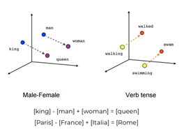
Now we have meaning between the vector so sending vectors means sending meaning in our embedded space. Let’s see an example to make it clear, here as we see if
king – man + woman = queen
In the above picture as we see the words having similar meanings are close to each other in embedded space. As we see in the example data is close to information as both carry similar information.
Word embedding mathematical works
We will take the input vector as a one-hot encoding vector. The product of input and embedding matrix and have an embedding vector.
How to train the model to have semantic relations between input and output vectors?
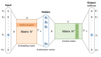
We will use a skip grant model where basically for an input word, we will pick several other words, which we called context and we want them to appear in the output vectors.
To create an output we need to have a large stack of sentences we will split the vectors. for each word, we will take two previous words and two next words as context.
Let’s take an example “In spite of everything. I still believe people are good at heart”. Word good produces pairs like (“good”, “are”), (“good”, “really”), (“good”, “at”), (“good”, “heart”) as a context.
Old fashioned sequence2sequence
Working
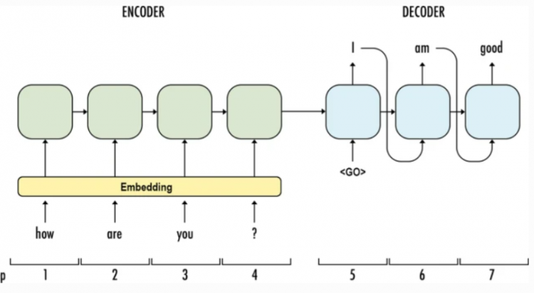
The encoder will summarize all the information that we want to use from the input sentences and the decoder will use it as inputs to create an output of the encoder in order to create the right output. The old method to do this with the help of Recurrent Neural Network RNN.
Steps to perform RNN
- First we will embed the words into vectors so they can be used more efficiently by algorithms.
- Each new state of the encoder is computed from the previous one and next word.
- The final stage of encoder passes the information to start decoding that we want to have from input sequence.
- Now we will apply decoders which uses the previous hidden state and output word to compute a new hidden state or word; in easy terms it’s like unrolling the information which we get from the encoder.
Limitations
- As we are not passing the whole sentence but only passing the words the essence of the sentence is not there or we will certainly loose the information from the begining of the sentence to each words we add.
- We could also loose the infomation which we loose at the encoding phase. To address this issue what we do is add attention mechanism.
Attention Mechanism in RNN
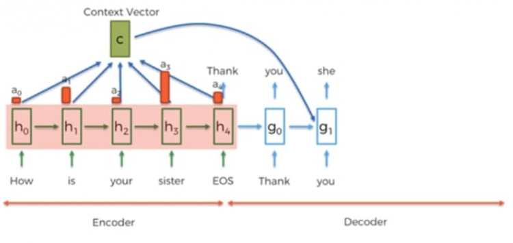
During the decoding phase, we add a new input to our cells in the RNN and then call the context vector and that’s vector will convey the information about the whole input sequence.
Let’s see an example suppose we are in the decoding phase at 2nd last word and we predicted the word she. We have a hidden state g1 and in parallel, we will compute the g2 by using a g1 hidden state and previous predicted word she and get the new word is.
But here, we added a new input, which is vector C that is created by hidden states of the encoder.
Now comes the question of how to send those hidden states? It’s represented by the coefficient, a zero and one, and so on. Hidden states, so how our current decoding phases is related to each of the encoding phases. So just having declared the subject is related to each of those hidden states and naturally. So that’s how the attention mechanism works in the RNN.
The mathematical equation for attention mechanism
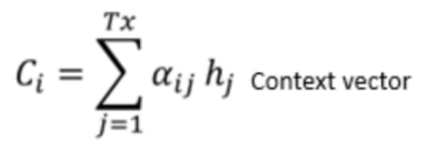
We use a softmax function in order to create weights for a weight. So the coefficients of being the similarity, for instance, between the state of our decoder and the hidden state of our encoder being those coefficients. Now we just need them to compute the alpha order to keep the relation between E.
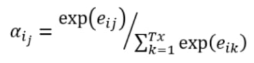
There is a direct proportion to the coefficients and alpha as one increases others one too increase. But as we are using softmax, the sum will be equal to one and each number will be between 0 and 1.
To see the similarity between the words we use a similarity function between the current hidden state and all of the hidden states of the encoder. As now we have similarity weights, we just need to apply a softmax function in order to have a real weight that we can use for weighted sums.
And we apply those weights to all the hidden states of the encoder to finally have a vector that is mostly made of the hidden states from the encoder that are related to our current state in the coding phase.
Transformers – Intutions
We saw how the attention mechanism works in RNN. There are some disadvantages too. The RNN is sequential processing so, it doesn’t have global behaviors concerning the input sequence and so we lose the important information along the coding process.
The fact that the large hidden state of the encoder, which is the final output of the encoder, has not seen the beginning of the sentences for quite a long time could make a disturbance in the model.
So for very long sentences or very long sequences, we lose a lot of information and that’s a huge demerit. Attention mechanism added the global behaviors to the coding phase, but the audience still has the weakness of not being global enough. Google introduced a paper called Attention which is most helpful here.
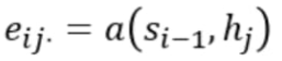
In the above picture, we have two main blocks; one on the left is an encoder and another one on right is the decoder. The change in the architecture is that our input for the encoder will be the whole sentences, so we don’t feed the input of the encoder single words.
The second main change is that the output of our decoders is a new input as we did before but now with the whole sentences. Here is the key we use inputs for our decoders is the one that we already had the previous iterations in the decoders. Additionally, the new words that we will predict at the end of this sequence
Summarizing the working
For example, when you have two sequences, it just composes the first sentence to how each element of the first sentence is related to the elements of the second sentence. Here, we use the same sentences three times, and actually that they call self-attention which is the key of the encoder in the transformer.
Before RNN we use standard neural networks, we have the information of the beginning of the sentences and then we add new words. We do the computation and we get the new information about the sentences.
But now we have whole sentences and we will see how each word of its sentences is related to the other words of the sentences then we will recompose these sentences according to that.
Let’s take an example “The animals didn’t cross the street because it was too tired”, here when we apply the attention mechanism it computes how each word of the sentence is related to the others. Here the word ‘it’ refers to animals that was too tired. When we see the output then the word it will produce a combination of strong words related to the sentence.
The goal of applying the self-protection mechanism is to combine everything so that each element doesn’t only represent the words but also represents the relation between the different words of sequences. This is the whole process of how self-attention works.
Mixing the information from the encoder according to how each element is related to this sequence from the decoder. We will see this in detail in the attention mechanism.
Attention in Tranformer
Till now we saw a general idea about transformers which is the base of the bert model.
Let’s say we have two sentences that can be equal in the case of self-attention, B will be the context and A will be the sequence that we want to really work with. This is the sequence that conveys the information that we want to rearrange in a certain way.
This can depend on the use case as supposing we are working with a translator there are changes that one sentence in is English another one is in French and another one in any other language. Now we want to apply the attention mechanism and check how sentence A is related to sentence B.
- So we want to arrange the information according to how each element of it is related to the elements from B. How to do it?
- Before doing the attention mechanism we have a beginning of sequence A and context B that will let us know how we manipulate N and outputs. We have a new sequence where each element will be a mix of elements from A sentence that are related to the B elements and not B words.
- So generally speaking B tells us how we will combine elments from A or in the case of the self attention and A tells us how we recobine a sentnece.
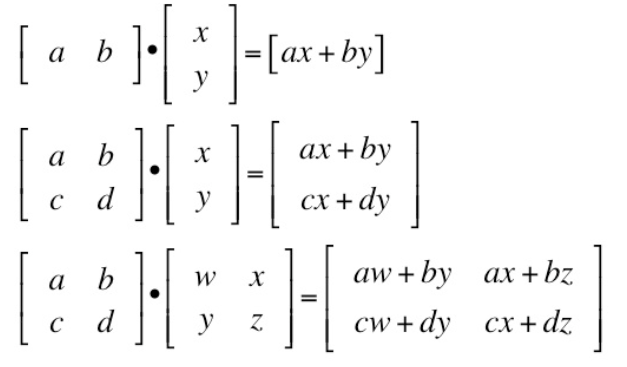
Dot product
The dot product is very useful to capture the similarities between two words. The way of computing the similarities focuses on the directions of the vectors.
- If the product = 1, there will be No correlation
- If the product = 0, there will be collated in an opposite manner if the other product is -ve one.
See in the below image the word joy and despair are the opposite words so they are in the opposite direction. so the dot product between joy and despair will be -1 and we see the word tree is not particularly related to joy and despair that’s why it’s perpendicular.

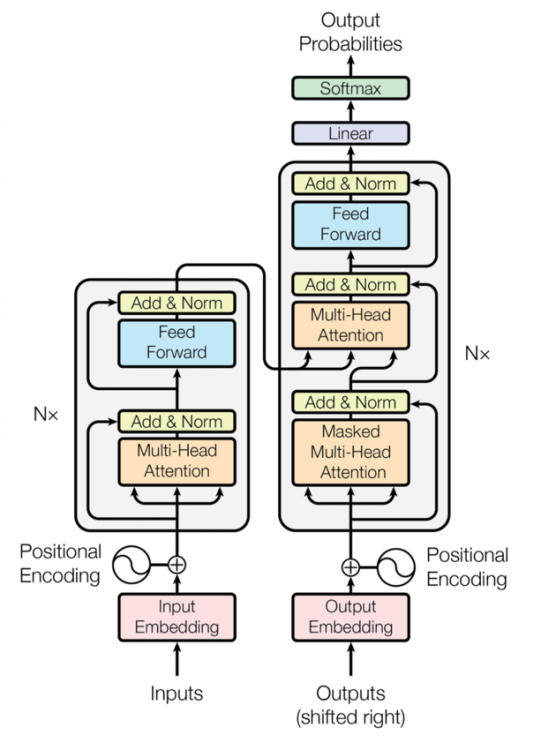
Now we see how the Dot product works, so we will be doing dot product of the A and B sentences. The below attached image explanation.
- Exmaple 1: Here, as we see left vector is horizontal and the right vector is vertical, and do the dot product.
- Exmaple 2: Here, as we see left is a matrix and the right vector is vertical, and doing the dot product we get whole matrix.
- Exmaple 3: Here, as we see left and right both are matrix, while doing dot product we get a matrix. This type of calculation is done when we want to compute many products at a time.
How to do scale dot product?
Let’s understand the formula first then moves to architecture.
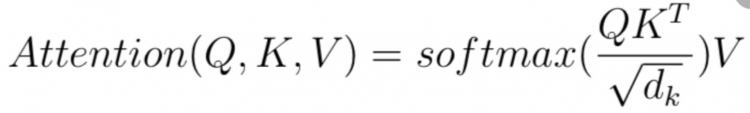
We have two sequences A and B which are K and V and Q will be the context.
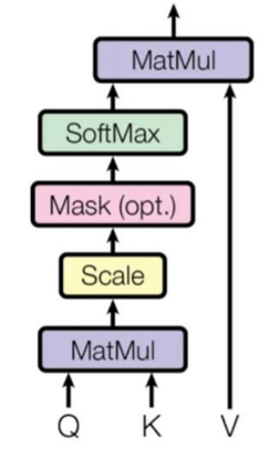
Steps to do
- Product of two Q and A where Q which is the context of the sentences with the A which is sequence and after the embedding, each sentence being a matrix, we get all the products that we wanted.
- Now we will do small scale it’s just something we need to do to improve the model and it stabilizes the whole process.
The next step is to apply softmax; softmax takes input as a vector and gives a vector with the same dimensions but each element will be between 0 and 1. The most important thing is we keep the relations between each element of the initial vectors.
- So now if element two was lower, then element three will be the same after the softmax.
- The second point of softmax is we just keep half each element is greater or lower than the others.
- The third point is that the sum of all the elements from the output of such max should be equal to 1, the reason fits the weights in mathematics.
- This shows that no information get out of hands just because the sum of quals 1. So this softmax is neceesary in order to get valid weights
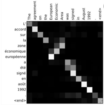
The below picture shows the A and B sentences similarity between the two words. As the range of black color increases the similarity between the words decreases, the whiter the color is, the more important the similarity between the words.
As we saw how the self-attention mechanism works.
So in this case, C and U would be equal to K and V, so the initial sentence and the context sentence are the same, which means that we will compose the sentence according to how each word of this sentence is related to the other words of this other sentences.
We repeat this process several times in the paper they say we do that eight times in order to make sure that we get the most out of this recomposition of the information. So in the training, we will have a pair of text or a pair of sentences.
Look ahead mask
During training, we feed a whole output sentence to the decoder, but to predict the word N, he must not look at the word N. Let’s change the attention matrix. We will change the self-protection mechanism when we compose the sentences there we will use the elements from the sentence, which are actually the starting token and the first AI minus one word.
Multi-head attention layer
Let’s understand how the mechanism works, scale dot product is not directly applied to the sentences. They first completed linear projects and after that they do concatenations. So instead of applying skills that predict attention to the whole sentences, they split each factor from the sentences.
Let’s take an example like each word after embedding has 12 dimensions, we will split into four sequences having three dimensions then we compute the scale that attention and can get the result in order to get back. Now attention mechanism can focus on these 3 dimensions so that the information is not faded into the 12 initial dimensions of the embedding.
Splitting the space into spaces allows the attention mechanism to attend to more information and to be able to get more relations between the elements of a sequence.
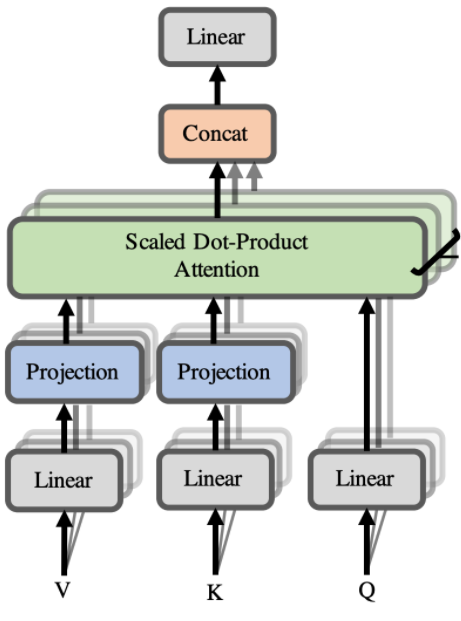
Mathematically
One big linear function is applied first and then a splitting allows each subspace to compose with the full original vector. Splitting and then applying a linear function restricts the possibilities.
Architecture
Bert is just a stack of simple encoder layers of the transformer which allows it to encode the sentences, encodes a language in the most effective way. So be composing information between every word of the sentence according to the relations between each other.
In the paper, Google talks about two different models that the choice that they implemented, the first one that they called Bert Base, and the second one which is bigger called Bert Large.
Hyperparameters used are:
- L – Number of encoder layers
- H – Hidden size
- A – Number of self-attention heads
The two models configuration
- Bert base: L=12, H=768, A=12, parameters: 110M
- Bert large: L=24, H=1024, A=16, parameters: 340M
The large module uses twice as many layers compares to the base model.
Bert’s input flexibility
We want our input to go in 2 ways; in single sentences and pairs of sentences. So instead of having one vector per word, we would like to have a vector that could be directly used for classification, that can summarize the whole sentences.
We want to have easy access to a classification tool: [CLS] + Sent A + [SEP] + Sent B
CLS: classification token
SEP: separation token between 2 sentences
How to give input to the best? We will convert the sentences into tokenization; here each token will be related to a number so our computer can understand easily. We can deal with the new words by combining known words and it will try to process the biggest word possible in order to decompose an unknown word.
If the word is just a bunch of nonsense, random letters, or numbers it will split the word into random letters.
tokenizer.tokenize('I am learning Transformer')

# Output
['i', 'am', 'learning', 'transform', '##er']
In the above code, the tokenization is done by splitting the words as we see the last word transformer; it’s not a common word that’s why the tokenizer splits the word into two words transform and er.
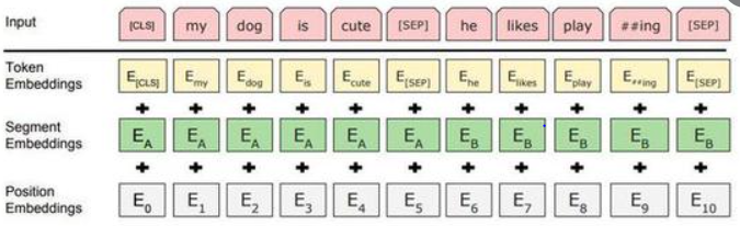
As we see in the above picture, taking input sentences and converting them into token embedding + segment embedding + position embedding.
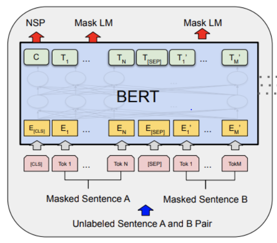
Outputs
We have two types of outputs one is single token C and another one is T the whole sequence.
- C is used for classification, trained during next sentence prediction. Classification task like spam detectors or sentimental analysis.
- T is used for the word-level tasks.
Final Conclusion
To conclude we saw that a single word in one hot encoding inversion gets a smaller vector and from the smaller vector, we get several words that are often close to the initial words of the corpus. We saw word embedding with the skip-gram module. The tokenizer which we used is a WordPiece tokenizer
Saw working on the Attention Mechanism of RNN and its advantages and disadvantages.
Transformer-intuitions here we are taking whole sentences and not words and their composing sequences, and making different sequences and see how they are related to each other, it’s just a way to extract global information from the sentences.
Trending Posts You Might Like
2020-02-11
11 minutes read
views
2276 words
How BERT works
BERT makes use of Transformer, an attention mechanism that learns contextual relations between words (or sub-words) in a text. In its vanilla form, Transformer includes two separate mechanisms — an encoder that reads the text input and a decoder that produces a prediction for the task. Since BERT’s goal is to generate a language model, only the encoder mechanism is necessary.
As opposed to directional models, which read the text input sequentially (left-to-right or right-to-left), the Transformer encoder reads the entire sequence of words at once. Therefore it is considered bidirectional, though it would be more accurate to say that it’s non-directional. This characteristic allows the model to learn the context of a word based on all of its surroundings (left and right of the word).
Bert + SQuAD

In Question Answering tasks (e.g. SQuAD v1.1), the software receives a question regarding a text sequence and is required to mark the answer in the sequence. Using BERT, a Q&A model can be trained by learning two extra vectors that mark the beginning and the end of the answer.

SQuAD v1.1:给定一个句子(通常是一个问题)和一段描述文本, 输出这个问题的答案, 类似于做阅读理解的简答题. 如图©表示的, SQuAD的输入是问题和描述文本的句子对. 输出是特征向量, 通过在描述文本上接一层激活函数为softmax的全连接来获得输出文本的条件概率, 全连接的输出节点个数是语料中Token的个数.
$P_i = frac{e^{V cdot C_i}}{sum^4_{j=1}e^{V cdot C_i}}$
Performance
On SQuAD v1.1, BERT achieves 93.2% F1 score (a measure of accuracy), surpassing the previous state-of-the-art score of 91.6% and human-level score of 91.2%:

For SQuAD2.0:

Input Formatting
Because BERT is a pretrained model that expects input data in a specific format, we will need:
- special tokens to mark the beginning ([CLS]) and separation/end of sentences ([SEP])
- tokens that conforms with the fixed vocabulary used in BERT
- token IDs from BERT’s tokenizer
- mask IDs to indicate which elements in the sequence are tokens and which are padding elements
- segment IDs used to distinguish different sentences
- positional embeddings used to show token position within the sequence

Special Tokens
BERT can take as input either one or two sentences, and expects special tokens to mark the beginning and end of each one:
- 2 Sentence Input:
[CLS] The man went to the store. [SEP] He bought a gallon of milk. [SEP]
- 1 Sentence Input:
[CLS] The man went to the store. [SEP]
Tokenization
BERT provides its own tokenizer. Let’s see how it handles the below sentence.
text = "Here is the sentence I want embeddings for."
marked_text = "[CLS] " + text + " [SEP]"

# Tokenize our sentence with the BERT tokenizer.
tokenized_text = tokenizer.tokenize(marked_text)

# Print out the tokens.
print (tokenized_text)
['[CLS]', 'here', 'is', 'the', 'sentence', 'i', 'want', 'em', '##bed', '##ding', '##s', 'for', '.', '[SEP]']
Notice how the word “embeddings” is represented:
['em', '##bed', '##ding', '##s']
The original word has been split into smaller subwords and characters. The two hash signs preceding some of these subwords are just our tokenizer’s way to denote that this subword or character is part of a larger word and preceded by another subword. So, for example, the ‘##bed’ token is separate from the ‘bed’ token; the first is used whenever the subword ‘bed’ occurs within a larger word and the second is used explicitly for when the standalone token ‘thing you sleep on’ occurs.
WordPiece
Why does it look this way? This is because the BERT tokenizer was created with a WordPiece model.
WordPiece原理

现在基本性能好一些的NLP模型,例如OpenAI GPT,google的BERT,在数据预处理的时候都会有WordPiece的过程.

WordPiece字面理解是把word拆成piece一片一片.

WordPiece的一种主要的实现方式叫做BPE(Byte-Pair Encoding)双字节编码.

BPE的过程可以理解为把一个单词再拆分,使得词表会变得精简,并且寓意更加清晰. 比如"loved","loving","loves"这三个单词. 其实本身的语义都是“爱”的意思,但是如果以单词为单位,那它们就算不一样的词,在英语中不同后缀的词非常的多,就会使得词表变的很大,训练速度变慢,训练的效果也不是太好。BPE算法通过训练,能够把上面的3个单词拆分成"lov","ed","ing","es"几部分,这样可以把词的本身的意思和时态分开,有效的减少了词表的数量.
This model greedily creates a fixed-size vocabulary of individual characters, subwords, and words that best fits our language data. Since the vocabulary limit size of our BERT tokenizer model is 30,000, the WordPiece model generated a vocabulary that contains all English characters plus the ~30,000 most common words and subwords found in the English language corpus the model is trained on. This vocabulary contains four things:
- Whole words
- Subwords occuring at the front of a word or in isolation (“em” as in “embeddings” is assigned the same vector as the standalone sequence of characters “em” as in “go get em” )
- Subwords not at the front of a word, which are preceded by ‘##’ to denote this case
- Individual characters
To tokenize a word under this model, the tokenizer first checks if the whole word is in the vocabulary. If not, it tries to break the word into the largest possible subwords contained in the vocabulary, and as a last resort will decompose the word into individual characters. Note that because of this, we can always represent a word as, at the very least, the collection of its individual characters.
As a result, rather than assigning out of vocabulary words to a catch-all token like ‘OOV’(Out-of-vocabulary) or ‘UNK’(Unknown), words that are not in the vocabulary are decomposed into subword and character tokens that we can then generate embeddings for.
So, rather than assigning “embeddings” and every other out of vocabulary word to an overloaded unknown vocabulary token, we split it into subword tokens [‘em’, ‘##bed’, ‘##ding’, ‘##s’] that will retain some of the contextual meaning of the original word. We can even average these subword embedding vectors to generate an approximate vector for the original word.
Here are some examples of the tokens contained in our vocabulary. Tokens beginning with two hashes are subwords or individual characters.
list(tokenizer.vocab.keys())[5000:5020]
['knight',
 'lap',
 'survey',
 'ma',
 '##ow',
 'noise',
 'billy',
 '##ium',
 'shooting',
 'guide',
 'bedroom',
 'priest',
 'resistance',
 'motor',
 'homes',
 'sounded',
 'giant',
 '##mer',
 '150',
 'scenes']
After breaking the text into tokens, we then have to convert the sentence from a list of strings to a list of vocabulary indeces.
Example
From here on, we’ll use the below example sentence, which contains two instances of the word “bank” with different meanings.
# Define a new example sentence with multiple meanings of the word "bank"
text = "After stealing money from the bank vault, the bank robber was seen "
       "fishing on the Mississippi river bank."

# Add the special tokens.
marked_text = "[CLS] " + text + " [SEP]"

# Split the sentence into tokens.
tokenized_text = tokenizer.tokenize(marked_text)

# Map the token strings to their vocabulary indeces.
indexed_tokens = tokenizer.convert_tokens_to_ids(tokenized_text)

# Display the words with their indeces.
for tup in zip(tokenized_text, indexed_tokens):
    print('{:<12} {:>6,}'.format(tup[0], tup[1]))
[CLS] 101 after 2,044 stealing 11,065 money 2,769 from 2,013 the 1,996 bank 2,924 vault 11,632 , 1,010 the 1,996 bank 2,924 robber 27,307 was 2,001 seen 2,464 fishing 5,645 on 2,006 the 1,996 mississippi 5,900 river 2,314 bank 2,924 . 1,012 [SEP] 102
Segment ID
BERT is trained on and expects sentence pairs, using 1s and 0s to distinguish between the two sentences. That is, for each token in “tokenized_text,” we must specify which sentence it belongs to: sentence 0 (a series of 0s) or sentence 1 (a series of 1s). For our purposes, single-sentence inputs only require a series of 1s, so we will create a vector of 1s for each token in our input sentence.
If you want to process two sentences, assign each word in the first sentence plus the ‘[SEP]’ token a 0, and all tokens of the second sentence a 1.
# Mark each of the 22 tokens as belonging to sentence "1".
segments_ids = [1] * len(tokenized_text)

print (segments_ids)
[1, 1, 1, 1, 1, 1, 1, 1, 1, 1, 1, 1, 1, 1, 1, 1, 1, 1, 1, 1, 1, 1]
Out-of-memory issues
All experiments in the paper were fine-tuned on a Cloud TPU, which has 64GB of device RAM. Therefore, when using a GPU with 12GB — 16GB of RAM, you are likely to encounter out-of-memory issues if you use the same hyperparameters described in the paper.
The factors that affect memory usage are:
- max_seq_length: The released models were trained with sequence lengths up to 512, but you can fine-tune with a shorter max sequence length to save substantial memory. This is controlled by the max_seq_length flag in our example code.
- train_batch_size: The memory usage is also directly proportional to the batch size.
- Model type, BERT-Base vs. BERT-Large: The BERT-Large model requires significantly more memory than BERT-Base.
- Optimizer: The default optimizer for BERT is Adam, which requires a lot of extra memory to store the m and v vectors. Switching to a more memory efficient optimizer can reduce memory usage, but can also affect the results. We have not experimented with other optimizers for fine-tuning.
Using the default training scripts (run_classifier.py and run_squad.py), we benchmarked the maximum batch size on single Titan X GPU (12GB RAM) with TensorFlow 1.11.0:

Unfortunately, these max batch sizes for BERT-Large are so small that they will actually harm the model accuracy, regardless of the learning rate used. We are working on adding code to this repository which will allow much larger effective batch sizes to be used on the GPU. The code will be based on one (or both) of the following techniques:
- Gradient accumulation: The samples in a minibatch are typically independent with respect to gradient computation (excluding batch normalization, which is not used here). This means that the gradients of multiple smaller minibatches can be accumulated before performing the weight update, and this will be exactly equivalent to a single larger update.
- Gradient checkpointing: The major use of GPU/TPU memory during DNN training is caching the intermediate activations in the forward pass that are necessary for efficient computation in the backward pass. “Gradient checkpointing” trades memory for compute time by re-computing the activations in an intelligent way.
Summary
SQuAD Example:
{
   "data":[
      {
         "title":"Super_Bowl_50",
         "paragraphs":[
            {
               "context":"Super Bowl 50 was an American football game to determine the champion of the National Football League (NFL) for the 2015 season. The American Football Conference (AFC) champion Denver Broncos defeated the National Football Conference (NFC) champion Carolina Panthers 24–10 to earn their third Super Bowl title. The game was played on February 7, 2016, at Levi\'s Stadium in the San Francisco Bay Area at Santa Clara, California. As this was the 50th Super Bowl, the league emphasized the "golden anniversary" with various gold-themed initiatives, as well as temporarily suspending the tradition of naming each Super Bowl game with Roman numerals (under which the game would have been known as "Super Bowl L"), so that the logo could prominently feature the Arabic numerals 50.",
               "qas":[
                  {
                     "answers":[
                        {
                           "answer_start":177,
                           "text":"Denver Broncos"
                        },
                        {
                           "answer_start":177,
                           "text":"Denver Broncos"
                        },
                        {
                           "answer_start":177,
                           "text":"Denver Broncos"
                        }
                     ],
                     "question":"Which NFL team represented the AFC at Super Bowl 50?",
                     "id":"56be4db0acb8001400a502ec"
                  }
               ]
            }
         ]
      }
   ],
   "version":"1.1"
}
Basic structure: [CLS]+query tokens+[SEP]+context tokens+[SEP]
- token_to_orig_map : Considering the index of each word as a feature integer
INFO:tensorflow:token_to_orig_map: 17:0 18:1 19:2 20:3 21:4 22:5 23:5 24:5 25:6 26:7 27:8 28:9 29:10 30:11 31:12 32:13 33:14 34:15 35:16 36:17 37:17 38:17 39:17 ...............................196:115 197:116 198:117 199:118 200:119 201:120 202:121 203:121 204:121 205:122 206:122 207:122 208:123 209:123
— 17 represents that the context tokens starts at 17th (before that, are [CLS]+query tokens+[SEP]
— 0 represents the first word, 1 represents the second word…
- token_is_max_context : A Boolean index to each word representing whether the word is important in the context or not.
INFO:tensorflow:token_is_max_context: 17:True 18:True 19:True 20:True 21:True 22:True 23:True 24:True 25:True 26:True 27:True 28:True 29:True 30:True 31:True 32:True ...........................202:True 203:True 204:True 205:True 206:True 207:True 208:True 209:True
— Boolean值表示该位置的token在当前span里面是否是最全上下文的
— E.g.Doc: the man went to the store and bought a gallon of milkbought在spanB和spanC里都有出现,但很显然span C里bought是语境最全的,既有上文也有下文
| Span A: the man went to the
| Span B: to the store and bought
| Span C: and bought a gallon of
- input_ids : Assigning word to vector ids to each word of context by considering the words dictionary data from pretrained BERT.
INFO:tensorflow:input_ids: 101 1134 183 2087 1233 1264 2533 1103 170 2087 1665 1120 7688 7329 1851 136 102 7688 7329 1851 1108 1126 1821 26237 1389 1709 1342 1106 4959 1103 3628 1104 1103 1569 1709 2074 113 183 2087 1233 114 1111 ............................ 0 0 0 0 0 0 0 0 0 0 0 0 0 0 0 0 0 0 0 0 0 0 0 0 0 0 0 0 0 0 0 0 0 0
- input_mask : Boolean mask to the context words based on their presence and followed by zero padding to meet the max word vector representation used for specific downloaded BERT model.
INFO:tensorflow:input_mask: 1 1 1 1 1 1 1 1 1 1 1 1 1 1 1 1 1 1 1 1 1 1 1 1 1 1 1 1 1 1 1 1 1 1 1 1 1 1 1 1 1 1 1 1 1 1 1 1 1 1 1 1 1 1 ............... 0 0 0 0 0 0 0 0 0 0 0 0 0 0 0 0 0 0 0 0 0 0 0 0 0 0 0 0 0 0 0 0 0 0 0 0 0 0 0 0 0 0 0 0 0 0 0
- segment_ids : segment ids to indicate whether a token belongs to the first sequence or the second sequence
INFO:tensorflow:segment_ids: 0 0 0 0 0 0 0 0 0 0 0 0 0 0 0 0 0 1 1 1 1 1 1 1 1 1 1 1 1 1 1 1 1 1 1 1 1 1 1 1 1 1 1 1 1 1 1 1 1 1 1 1 1 1 1 1 1 1 1 1 1 1 1 1 1 1 1 1 1 1 1 1 1 1 1 1 1 1 1 1 1 1 1 1 1 1 1 1 1 1 1 1 1 1 1 1 1 1 1 1 1 1 1 1 1 1 1 1 1 .............0 0 0 0 0 0 0 0 0 0 0 0 0 0 0 0 0 0 0 0 0 0 0 0 0 0 0 0 0 0
References
- SQuAD
- BERT-word-embeddings
- http://jalammar.github.io/a-visual-guide-to-using-bert-for-the-first-time/
- Bert+SQuAD_Chatbot
- https://www.jianshu.com/p/43e8f186e03a
- BERT-WordPiece
- SQuAD fine-tune source code analysis
- run_squad.py
- https://carlos9310.github.io/2019/09/27/MRC-squad2.0/
- cdqa
Перевод
Ссылка на автора

Несомненно, исследование Natural Language Processing (NLP) сделало огромный скачок после того, как оно оставалось относительно стационарным в течение нескольких лет. Во-первых, двунаправленные представления кодировщиков Google от Transformer (BERT) [1] стали основным моментом к концу 2018 года для достижения современного уровня производительности во многих задачах НЛП и не намного позже, GPA-2 OpenAI ворует гром, обещая еще более удивительные результаты, которые, по сообщениям, делают его слишком опасным для публикации! Принимая во внимание временные рамки и игроков, стоящих за этими публикациями, не требуется никаких усилий, чтобы понять, что в данный момент в пространстве много активности.
При этом мы сконцентрируемся на BERT для этого поста и попытаемся получить небольшой кусочек этого пирога путем извлечения предварительно обученных контекстуализированных вложений слов, таких как ELMo [3].
Чтобы дать вам краткое описание, я сначала немного расскажу о фоновом контексте, затем кратко расскажу об архитектуре BERT и расскажу о коде, объясняя некоторые хитрые части здесь и там.
Просто для большего удобства я буду использовать Colab от Google для кодирования, но этот код может также работать в вашей локальной среде без многих модификаций.
Если вы пришли только для части кода, перейдите к «BERT Word Embedded Извлечение» раздел. Найти готовый код ноутбука Вот,
Вложения слов
Для начала, вложения — это просто (умеренно) низкоразмерные представления точки в векторном пространстве более высокого измерения. Точно так же вложения слов представляют собой плотные векторные представления слов в пространстве нижних измерений. Первая модель внедрения слов с использованием нейронных сетей была опубликована в 2013 году [4] исследованием в Google. С тех пор вложения слов встречаются практически во всех моделях НЛП, используемых сегодня на практике. Конечно, причина такого массового усыновления — откровенно говоря, их эффективность. Переводя слово во вложение, становится возможным смоделировать семантическую значимость слова в числовой форме и, таким образом, выполнить математические операции над ним. Чтобы сделать это более ясным, я приведу наиболее распространенный пример, который вы можете найти в контексте встраивания слов

Когда это впервые стало возможным благодаря модели word2vec, это был удивительный прорыв. Оттуда появилось много более продвинутых моделей, которые не только уловили статический смыслконтекстуализированное значение, Например, рассмотрим два предложения ниже:
Я люблю яблоки.
Мне нравятся яблочные макбуки
Обратите внимание, что слово «яблоко» имеет различное семантическое значение в каждом предложении. Теперь с контекстуализированной языковой моделью встраивание слова apple будет иметь другое векторное представление, что делает его еще более мощным для задач НЛП.
Тем не менее, я оставлю детали того, как это работает, за рамками этого поста, просто чтобы он был кратким и точным.
трансформеры
Честно говоря, большая часть прогресса в области НЛП может быть приписана успехам общих исследований в области глубокого обучения. В частности, Google (снова!) Представил новую архитектуру нейронной сети, названную трансформатором в оригинальной статье [5], которая имела много преимуществ по сравнению с обычными последовательными моделями (LSTM, RNN, GRU и т. Д.). Преимущества включали, но не ограничивались, более эффективное моделирование долгосрочных зависимостей между токенами во временной последовательности и более эффективное обучение модели в целом за счет устранения последовательной зависимости от предыдущих токенов.
В двух словах, преобразователь — это модель архитектуры кодер-декодер, которая использует механизмы внимания, чтобы направлять более полное изображение всей последовательности сразу в декодер, а не последовательно, как показано на рисунках ниже.

Опять же, я не буду описывать детали того, как работает внимание, поскольку это сделает тему более запутанной и более трудной для восприятия. Не стесняйтесь следовать соответствующей статье в ссылках.
GPT OpenAI был первым, кто создал модель языка на основе преобразователя с тонкой настройкой, но, если быть более точным, он использовал только декодер преобразователя. Поэтому, делаямоделирование языка однонаправленное, Техническая причина отказа от кодера заключалась в том, что моделирование языка стало бы тривиальной задачей, так как слово, которое было предсказано, могло в конечном итоге увидеть себя.
Двунаправленные представления кодировщика от Transformer (BERT)
К настоящему времени название модели, вероятно, должно иметь больше смысла и дать вам приблизительное представление о том, что это такое. BERT свел все воедино, чтобы построить двунаправленную языковую модель на основе преобразователя, используя кодеры, а не декодеры! Чтобы преодолеть проблему «видеть себя», у ребят из Google была гениальная идея. Они работалимоделирование языка масок Другими словами, они спрятали 15% слов и использовали информацию о своем положении, чтобы вывести их. Наконец, они также немного перепутали, чтобы сделать процесс обучения более эффективным.
Хотя эта методология оказала негативное влияние на время конвергенции,это превзошло современные моделиеще до конвергенции, которая опечатала успех модели.
Обычно BERT представляет собой общее языковое моделирование, которое поддерживает трансферное обучение и тонкую настройку для конкретных задач, однако в этом постемы только коснемся стороны извлечения возможностей BERT, просто получив из нее ELMo-подобные вложения слов, используя Keras и TensorFlow.
Но держи лошадей! Прежде чем мы углубимся в код, давайте очень быстро исследуем архитектуру BERT, чтобы у нас было немного опыта во время реализации. Поверьте мне, это намного облегчит понимание.
Фактически разработчики BERT создали две основные модели:
- БАЗА:Количество блоков трансформатора (L): 12, Размер скрытого слоя (H): 768 и Внимание внимание (A): 12
- LARGE:Количество блоков трансформатора (L): 24, Размер скрытого слоя (H): 1024 и Внимание (A): 16
В этом посте я буду использовать модель BASE, поскольку ее более чем достаточно (и намного меньше!).
С точки зрения очень высокого уровня архитектура BERT выглядит следующим образом:

Это может показаться простым, но помните, что каждый блок кодера содержит более сложную модель архитектуры.
На этом этапе, чтобы прояснить ситуацию, важно понимать специальные токены, которые авторы BERT использовали для тонкой настройки и обучения конкретным задачам. Это следующие:
- [ЦБС]: Первый токен каждой последовательности. Жетон классификации, который обычно используется вместе со слоем softmax для задач классификации. Для всего остального это можно смело игнорировать.
- [Сентября]: Токен разделителя последовательностей, который использовался при предварительном обучении для задач пары последовательностей (т. Е. Предсказание следующего предложения). Должен использоваться, когда требуются пары последовательностей. Когда используется одна последовательность, она просто добавляется в конце.
- [МАСКА]:Токен используется для замаскированных слов. Используется только для предварительной подготовки.
Далее, формат ввода, который ожидает BERT, показан ниже:

Таким образом, любой ввод, который будет использоваться с BERT, должен быть отформатирован в соответствии с вышеприведенным.
входной слойэто просто вектор последовательности токенов вместе со специальными токенами. «## ИНГ»токен в приведенном выше примере может поднять некоторые брови, поэтому, чтобы уточнить, BERT использует WordPiece [6] для токенизации, которая в действительности разделяет токен, например, «игра» на «игра» и «## ing». Это в основном для охвата более широкого спектраВне Словаря (OOV)слова.
Встраивание токеновявляются словарными идентификаторами для каждого из токенов.
Предложения вложенияэто просто числовой класс, чтобы различать предложения A и B.
И наконец,Трансформаторные позиционные вложенияуказать положение каждого слова в последовательности. Более подробную информацию об этом можно найти в [5].
Наконец, есть еще одна вещь. Все отлично, это мягко, но как я могу получить вложения слов от этого?!? Как уже говорилось, базовая модель BERT использует 12 уровней трансформаторных кодеров,каждый вывод для каждого токена из каждого их слоя может использоваться как вложение слова!Вы, наверное, удивляетесь,какой из них лучший хотя?Ну, я думаю, это зависит от задачи, но эмпирически авторы определили, что одним из лучших вариантов выбора былосуммировать последние 4 слоя,что мы будем делать,

Как показано, наиболее эффективный вариант — объединить последние 4 слоя, но в этом посте подход суммирования используется для удобства. В частности,разница в производительности не так уж много, а также естьбольше гибкости для дальнейшего усечения размеров,не теряя много информации.
BERT Word Embedded Извлечение
Хватит теории. Давайте перейдем к практике.
Во-первых, создать новый Google Colab блокнот. Перейти кEdit-> НоутбукиНастройте и убедитесь, что аппаратный ускоритель установлен на TPU.

Теперь первая задача — клонировать официальный репозиторий BERT, добавить его каталог в путь и импортировать оттуда соответствующие модули.
!rm -rf bert
!git clone https://github.com/google-research/bertimport syssys.path.append('bert/')from __future__ import absolute_import
from __future__ import division
from __future__ import print_functionimport codecs
import collections
import json
import re
import os
import pprint
import numpy as np
import tensorflow as tfimport modeling
import tokenization
Два модуля, импортированные из BERT,моделированиеа такжелексический анализ, Моделирование включает в себя реализацию модели BERT, и токенизация, очевидно, предназначена для токенизации последовательностей.
В дополнение к этому мы получаем наш адрес TPU из colab и инициализируем новый сеанс тензорного потока. (Обратите внимание, что это относится только к Colab. При локальном запуске это не требуется). Если вы видите какие-либо ошибки при запуске блока ниже, убедитесь, что вы используете TPU в качестве аппаратного ускорителя (см. Выше)
Двигаясь дальше, мы выбираем, какую модель BERT мы хотим использовать
Как вы можете видеть, есть три доступные модели, которые мы можем выбрать, но на самом деле, есть еще больше предварительно обученных моделей, доступных для загрузки в официальном репозитории BERT GitHub. Это только те модели, которые уже были загружены и размещены Google в открытом ведре, так что к ним можно получить доступ из Colab Laboratory. (Для локального использования вам необходимо скачать и извлечь предварительно обученную модель).
Напомним параметры из ранее: 12 л (блоки трансформатора) 768 H (размер скрытого слоя) 12 A (головы внимания). «Uncased» только для строчных последовательностей. В этом примере мы будем использовать необработанную модель BERT BASE.
Кроме того, мы определяем некоторые глобальные параметры для модели:
Большинство приведенных выше параметров говорят сами за себя. На мой взгляд, единственное, что может быть немного сложнее, это массив LAYERS. Напомним, что мы используем на последних 4 слоях из 12 скрытых кодеров. Следовательно, LAYERS сохраняет свои индексы.
Следующая часть предназначена исключительно для определения классов-оболочек для ввода перед обработкой и после обработки (Возможности).
вInputExampleкласс, мы установилиtext_bвНиктопо умолчанию, поскольку мы стремимся использовать отдельные последовательности, а не пары последовательностей.
Кроме того,InputFeaturesКласс инкапсулирует функции, которые нужны BERT для ввода (см. схему ввода выше).жетонысвойство явно вектор входных токенов,input_idsявляются идентификаторы, которые соответствуют токену из словаря,Маска вводааннотирует реальную последовательность токенов от заполнения и, наконец,input_type_idsотделяет сегмент A от сегмента B, так что это не очень важно здесь.
Теперь добавьте следующий код:
Это настроить наш оценщик. Оценщик — это просто абстракция для модели, которую предоставляет тензорный поток вместе с API для обучения, оценки и прогнозирования. Таким образом, наша пользовательская оценка — это обертка вокруг BertModel. По общему признанию есть части кода, которые могут быть удалены из вышеупомянутого, но я придерживаюсь примера, который Google предоставил только для последовательности. Важные части есть линия 60 — где определена модель Берта — илиния 100где прогнозы из верхних 4 слоев извлекаются.
Продолжите, добавив также следующее:
Это функция, которая заботится о обработке ввода. Другими словами, это превращаетInputExamplesвInputFeatures,
В дополнение к этому мы создаем функцию для преобразования нормальной последовательности строк вInputExample:
Теперь для последнего бита кода мы определим функцию, которая принимает массив строк в качестве параметра и желаемое измерение (максимум 768) выходных данных для встраивания и возвращает словарь с токеном в качестве ключа и вектором встраивания в качестве значения.
Приведенный выше фрагмент кода просто строит оценщик и вызывает прогноз на основе заданных входных данных.
Давайте продолжим и протестируем нашу модель, выполнив это:
embeddings = get_features([“This is a test sentence”], dim=50)
print(embeddings)
Если все пойдет хорошо, у вас будет словарь, содержащий вложения размером 50 на токен. Помните, что это контекстные вложения, поэтому, если у вас есть дубликаты токенов на разных последовательностях, в словаре останется только вложение последнего токена. Чтобы сохранить оба, замените словарь другой структурой данных.
Вы можете найти полный блокнот Вот,
Будущая работа
Теперь эти вложения можно использовать в качестве входных данных для других моделей, созданных для пользовательских задач. Тем не менее, я оставлю это для другого поста. Или даже возможно реализовать BERT Keras Layer для бесшовной интеграции встраивания.
Вывод
Это все от меня, ребята. Надеюсь, вам понравился пост и, надеюсь, вы получили более четкое представление о BERT. Не стесняйтесь оставлять свои отзывы или вопросы в разделе комментариев.
Ссылки:
[1] Дж. Девлин, М. Чанг, К. Ли и К. Тутанова, BERT: предварительная подготовка глубинных двунаправленных трансформаторов для понимания языка (2018)
[2] Рэдфорд, Алек, Ву, Джефф, Чайлд, Ревон, Луан, Дэвид, Амодей, Дарио, Суцкевер, Илья, Языковые модели являются многозадачными учениками без присмотра (2019)
[3] М. Петерс, М. Нейман, М. Айер, М. Гарднер, К. Кларк, К. Ли и Л. Цеттлемойер, Глубокие контекстуальные представления слов (2018), Североамериканское отделение Ассоциации компьютерной лингвистики
[4] Т. Миколов, И. Сутскевер, К. Чен, Г. Коррадо и Дж. Дин, Распределенные представления слов и фраз и их композиционность (2013)
[5]. Васвани, Н. Шазир, Н. Пармар, Дж. Ускорейт, Л. Джонс, А. Гомес, Л. Кайзер и И. Полосухин, Внимание это все что вам нужно (2017)
[6] Й. У, М. Шустер, З. Чен, К. Ле, М. Норузи, В. Мачери, М. Крикун, Ю. Цао, К. Гао, К. Мачери, Дж. Клингнер, А. Шах , М. Джонсон, X. Лю, Ł. Кайзер, С. Гоус, Ю. Като, Т. Кудо, Х. Казава, К. Стивенс, Г. Курьян, Н. Патил, В. Ван, С. Янг, Дж. Смит, Дж. Риза, А. Рудник, О. Виньялс, Г. Коррадо, М. Хьюз и Дж. декан Система нейронного машинного перевода Google: преодоление разрыва между человеком и машинным переводом (2016)