
Пакет Wordcloud в Python помогает нам узнать частоту появления слова в текстовом контенте с помощью визуализации.
Чтобы реализовать это, нам нужно сначала установить некоторые пакеты, такие как pandas, matplotlib и Wordcloud. Давайте посмотрим на этапы установки каждого.
Установка Pandas
Pandas – отличный инструмент для реализации анализа и визуализации данных в Jupyter Notebook. Его можно импортировать в наш исходный код следующим образом:
import pandas as pd
PD относится к процессу создания псевдонимов, с помощью которого могут быть созданы фреймы данных, и это упрощает читаемость кода.
Pandas можно установить двумя способами:
- Использование командной строки.
Давайте посмотрим, как мы можем установить pandas с помощью командной строки:
- Открыть командную строку.
- Ввести данную команду:pip install pandas
- После нажатия «Enter» пакеты начнут загружаться в систему.
Эту же команду можно использовать в Linux в терминале для установки pandas в нашей системе.
- С помощью Anaconda Navigator.
Второй способ установить pandas – использовать Anaconda Navigator.
- Откройте Anaconda Navigator.
- Щелкните вкладку «Среда» и перейдите к параметру создания, чтобы настроить Pandas в вашей системе.
- Нажмите на кнопку «Создать» для среды Pandas.
- В списке пакетов выберите «Все», чтобы получить фильтры.
- Перейдите в строку поиска, найдите «Pandas» и выберите «Pandas package».
- Щелкните правой кнопкой мыши флажок и выберите «Отметить для установки определенной версии».
- Выберите версию, которую хотите установить, и нажмите кнопку «Применить», чтобы установить пакеты.

Установка Matplotlib
Matplotlib – обширная и интересная библиотека для людей, которые с энтузиазмом относятся к выводам результатов из данных, включает в себя диаграммы рассеяния, гистограммы, коробчатые диаграммы и многое другое, что упрощает нам понимание.
Matplotlib можно установить, выполнив следующие действия:
- Использование командной строки.
Matplotlib можно установить в нашей системе с помощью данной команды в командной строке:
pip install matplotlib
- Использование Anaconda.
Мы можем установить matplotlib с помощью Anaconda, набрав следующую команду в Anaconda Prompt:
conda install matplotlib

Проверка установки
Мы можем проверить, успешно ли установлен matplotlib в нашей системе или нет, набрав данную программу в терминале.
import matplotlib
matplotlib.__version__
Как обсуждалось ранее, это дает нам представление о наиболее часто встречающихся словах в тексте с помощью визуального элемента.
WordCloud можно установить, выполнив следующие действия:
- с помощью данной команды в командной строке:
pip install wordcloud
- Используя Anaconda, ввести следующую команду в строке:
conda install -c conda-forge wordcloud
Теперь давайте посмотрим на простую программу, которая показывает, как wordcloud можно использовать в Python.
Мы взяли этот фрагмент текста с веб-сайта и сохранили как файл sunflowers1.txt.
sunflowers1.txt
"Sunflowers are heliotropic, which means that they turn their flowers to follow the movement of the Sun across the sky east to west, and then returns at night to face the east, ready again for the morning sun. Heliotropism happens during the earlier stages before the flower grows heavy with seeds.
There are tons of varieties of sunflowers available today, so there's bound to be one that fits your garden. Choose between those with branching stems or single stems, those that produce ample pollen for pollinators or are pollen-free(best for bouquets), those that stay small or tower above the rest of the garden, or those that produce edible seeds! "
Реализация кода:
import re
import matplotlib.pyplot as plt
from wordcloud import WordCloud, STOPWORDS
text = open("/content/sunflowers1.txt", "r").read()
# Clean text
text = re.sub(r'==.*?==+', '', text)
text = text.replace('n', '')
# Define a function to plot word cloud
def plot_cloud(wordcloud):
    # Set figure size
    plt.figure(figsize=(40, 30))
    # Display image
    plt.imshow(wordcloud)
    # No axis details
    plt.axis("off")
# Generate word cloud
wordcloud = WordCloud(width = 3000, height = 2000, random_state=1, background_color='salmon', colormap='Pastel1', collocations=False, stopwords = STOPWORDS).generate(text)
plot_cloud(wordcloud)
Выход:


Изучаю Python вместе с вами, читаю, собираю и записываю информацию опытных программистов.

word_cloud
A little word cloud generator in Python. Read more about it on the blog
post or the website.
The code is tested against Python 2.7, 3.4, 3.5, 3.6 and 3.7.
Installation
If you are using pip:
pip install wordcloud
If you are using conda, you can install from the conda-forge channel:
conda install -c conda-forge wordcloud
Installation notes
wordcloud depends on numpy and pillow.
To save the wordcloud into a file, matplotlib can also be installed. See examples below.
If there are no wheels available for your version of python, installing the
package requires having a C compiler set up. Before installing a compiler, report
an issue describing the version of python and operating system being used.
Examples
Check out examples/simple.py for a short intro. A sample output is:
Or run examples/masked.py to see more options. A sample output is:
Getting fancy with some colors:
Generating wordclouds for Arabic:
Command-line usage
The wordcloud_cli tool can be used to generate word clouds directly from the command-line:
$ wordcloud_cli --text mytext.txt --imagefile wordcloud.png
If you’re dealing with PDF files, then pdftotext, included by default with many Linux distribution, comes in handy:
$ pdftotext mydocument.pdf - | wordcloud_cli --imagefile wordcloud.png
In the previous example, the - argument orders pdftotext to write the resulting text to stdout, which is then piped to the stdin of wordcloud_cli.py.
Use wordcloud_cli --help so see all available options.
Licensing
The wordcloud library is MIT licenced, but contains DroidSansMono.ttf, a true type font by Google, that is apache licensed.
The font is by no means integral, and any other font can be used by setting the font_path variable when creating a WordCloud object.
Wordclouds are a quick, engaging way to visualise text data. In Python, the simplest and most effective way to generate wordclouds is through the use of the Wordcloud library. In this tutorial, I’ll explain how to generate wordclouds using the Wordcloud library, showing how to customise and improve your visualisations.
This tutorial was written using using Jupyter notebooks, Python 3.7.5 and Wordcloud 1.6.0; things might behave slightly differently if you’re in a different IDE or using different versions of the language/library.
You can find a complete copy of the code for this tutorial on Github, along with the text data and images used throughout.
Disclaimer
Every statistician I have ever met requires me to inform you that wordclouds are not useful for analysis because they are simplistic and often misleading; I recommend this excellent article which goes into more detail on the problems with the form.
The criticisms of wordclouds are absolutely valid, but that’s not to say that wordclouds are pointless. While I wouldn’t recommend them as a method of analysis or information extraction, they’re a useful tool for presentation — people seem to find them fun and engaging, and they’re a good thing to have on initial pages of presentations, etc. As long as you focus on using them for aesthetic, rather than analytic, reasons, they have a place.
Data source
In order to demonstrate the possibilities of wordclouds, some text data is required. For the purposes of this tutorial, I’ve chosen to use the text of Addie’s Husband or Through Clouds to Sunshine, a novel by Mrs. Gordon Smythies, one of the most popular and most forgotten of Victorian novelists.
You can find a copy of Addie’s Husband on Amazon or on Project Gutenberg. It’s the affecting story of Adelaide, a young woman with bad lungs but a good heart. I accessed the text from Project Gutenberg, using the excellent Gutenberg Python library.
In order that this tutorial can focus almost entirely on wordclouds, rather than text cleaning, I’ve already processed the novel’s full text into a more consistent form. To be specific, the following steps have been carried out:
- Removal of all metadata, including chapter headings, leaving just the prose
- Conversion of all text to lowercase
- Removal of all punctuation, special characters, and numeric values
- Removal of stopwords and all words with fewer than 3 letters
- Lemmatisation (converting each word to its dictionary form)
- Removal of all proper nouns I found on a cursory search
The end result of this process is a text file — adelaide.txt — containing a standardised and simplified form of Addie’s Husband.
Required libraries
In order to work with the Wordcloud library effectively, you require several imports. Obviously the Wordcloud library itself, but also it helps to have libraries to deal with text processing and images.
from collections import Counter  # Count the frequency of distinct strings
from wordcloud import WordCloud, ImageColorGenerator  # Generate wordclouds
from PIL import Image  # Load images from files
import numpy as np  # Convert images to numbers
Enter fullscreen mode
Exit fullscreen mode
Loading and preparing the data
As already mentioned, the data for this tutorial is stored in a .txt file. The first step is simply to load the file’s data.
# Load the data from a file
with open("./resources/adelaide.txt", "r") as file:
    text = file.read()

# View the first 200 characters of the text

text[:200]
Enter fullscreen mode
Exit fullscreen mode
‘soldier sailor tinker tailor policeman plowboy gentleman lift lovely head dear marry gentleman miss absorbed enjoyment ruddy ribstone pippin turn blooming freckle face speaker answer pleasantly though’
Our current text is perfectly suitable for wordcloud generation — given raw text, the Wordcloud library will automatically process it and generate a wordcloud.
However, text can also be provided in the form of a frequency dictionary, in which the key:value pairs have the form word:frequency. I find this conceptually neater, as it allows you more explicit control over the processing steps before generating the cloud.
# Split the text into a list of individual words

tokens = text.split(" ")

# Count the frequency of each word

word_counts = Counter(tokens)

# Display the count for a single word.

word_counts["love"]
Enter fullscreen mode
Exit fullscreen mode
133
Basic wordclouds
In order to generate and display the most basic of wordclouds, very little is required. You need a WordCloud object, and then to call .generate() on it, passing a string as an argument.
Finally, to display the cloud, .to_image().
fog_machine = WordCloud()  # Create a wordcloud generator

fog_machine.generate(text)  # Generate the cloud using raw text

fog_machine.to_image()
Enter fullscreen mode
Exit fullscreen mode

Our basic wordcloud is rather small, and will require some customisation to improve.
In the code below, I’ve generated a slightly better one, by using the following parameters:
-
widthandheightto increase the size of the cloud’s canvas area, and thus image quality -
min_font_sizeto ensure that no words are too small to read -
background_colorto demonstrate that it doesn’t have to be black if you don’t want it to -
colormapto choose a specific colour palette. Any valid Matplotlib colormap name is acceptable.
I’ve also chosen to generate the cloud using the frequency dictionary this time, not the raw text; that doesn’t really have an effect on the style, it’s just to demonstrate how you would do it.
# Create a wordcloud generator with some better defaults

fog_machine = WordCloud(width=800,
                        height=600,
                        min_font_size=14,
                        background_color="#333333",
                        colormap="spring")

# Generate the cloud using a frequency dictionary

fog_machine.generate_from_frequencies(word_counts)

fog_machine.to_image()  # Display the cloud
Enter fullscreen mode
Exit fullscreen mode

It’s not the best thing ever — I don’t really have much of a talent for visual design — but I think it’s clearly an improvement.
Shaped wordclouds
Once you can create wordclouds with whatever colours you like, the next step is to shape the wordcloud, changing it from a boring rectangle into something appropriate to the content.
This is done by using an image as a mask; you provide the WordCloud object a numerical representation of an image with a white background, and the wordcloud will only draw words in positions where the image is not white.
As Addie’s Husband is a romance, it seems appropriate that the mask we use should be a heart. The image I’m using was sourced from Template Trove.
image = Image.open("./resources/heart.jpg")  # Load the image from a file

image  # Display the image
Enter fullscreen mode
Exit fullscreen mode

Once the image is loaded in, we need to convert it into a numeric form, in which each pixel is represented as an array of three integers; the WordCloud object will then only draw words on top of pixels in the image which are not equal to [255, 255, 255].
mask = np.array(image)  # Convert the image to a numeric representation (a 3D array)

mask[0][0]  # Display the top left pixel of the mask, which is white
Enter fullscreen mode
Exit fullscreen mode
array([255, 255, 255], dtype=uint8)
After creating the mask, you create the wordcloud almost exactly as before, just passing in the mask parameter.
One key point to note is that masked wordclouds ignore the width and height parameters, instead sizing themselves based on the dimensions of the mask, so there is no need to include them.
# Create a wordcloud generator with a mask

fog_machine = WordCloud(mask=mask,
                        min_font_size=14,
                        colormap="Reds")

# Generate the cloud using a frequency dictionary

fog_machine.generate_from_frequencies(word_counts)

fog_machine.to_image()  # Display the cloud
Enter fullscreen mode
Exit fullscreen mode

Shaping wordclouds like this works best with simple images, as otherwise the core shape is not clear. By default, it also only works with images that have a fully white background — transparent backgrounds, for example, are treated as non-masked, and the wordcloud occupies the full rectangle again.
It is possible to convert any image so that it has the correct structure for wordclouds, but doing so is rather beyond the scope of this tutorial; we’re focused on wordclouds today, not image processing.
Shaped & Coloured wordclouds
We can both shape and colour a wordcloud based on an image, so that the words not only form the rough shape, but that each word is coloured as the image is in the same place. For this task, we’ll use another heart, this one rainbow-coloured, and sourced from PNGfuel.
It’s important to note here that this is a relatively crude fitting — a word that spans across several colour changes on the image will still only be in one colour, and you’re not going to get lines as crisp and clear as the image itself. Again, this works best with simple images, ideally with clearly contrasting colours.
The first step is to load in an image, as before.
image = Image.open("./resources/rainbow_heart.jpeg")  # Load the image from a file

mask = np.array(image)  # Convert the image to a numeric representation

image  # Display the image
Enter fullscreen mode
Exit fullscreen mode

Once you’ve created the mask, you can then use it as an input to the ImageColorGenerator class, which is also part of the WordCloud library. This generates colours based on an image, and then can be used to colour words to match.
image_colours = ImageColorGenerator(mask)
Enter fullscreen mode
Exit fullscreen mode
You can then pass the ImageColorGenerator to a WordCloud object using the color_func parameter.
In order to ensure that our wordcloud roughly matches the colours of the image, I’ve set the max_words argument to 2000. This means that the WordCloud object will use more words than the default of 200, which will result in smaller words and — hopefully — clearer bands of colour.
# Create a wordcloud generator with a mask

fog_machine = WordCloud(mask=mask,
                        max_words=2000,
                        color_func=image_colours)

# Generate the cloud using a frequency dictionary

fog_machine.generate_from_frequencies(word_counts)

fog_machine.to_image()  # Display the cloud
Enter fullscreen mode
Exit fullscreen mode

Custom colour functions
It is sometimes useful to have full control over the colours of words, so that you can highlight particular words or groups of word; you might, for example, wish to show positive words in one colour and negative words in another.
We can define a custom colour function to do this, passing it to the color_func parameter just as for mask colours. In the code below, I’ve defined a very simple one — return gold for words with the letter «o» in, grey for every other word — but you can customise this function to do whatever you want.
When the WordCloud object calls the function, it passes it a lot of information; this means that — when defining your custom function — it’s better to have the parameters as *args, *kwargs, as then you can pick and choose which arguments to later care about. The word itself is always passed as the first argument, or args[0].
# The custom function

def custom_colours(*args, **kwargs):
    word = args[0]  # First argument is the word itself
    if "o" in word:
        return "#FFD700"
    return "#CCCCCC"

# Create a wordcloud generator with a custom color_func

fog_machine = WordCloud(width=800,
                        height=600,
                        min_font_size=14,
                        color_func=custom_colours)

# Generate the cloud using a frequency dictionary

fog_machine.generate_from_frequencies(word_counts)

fog_machine.to_image()  # Display the cloud
Enter fullscreen mode
Exit fullscreen mode
Saving wordclouds
You can save a wordcloud to a file with a single line of code.
fog_machine.to_file("wordcloud.png")
Enter fullscreen mode
Exit fullscreen mode
The header image
The header image for this tutorial was generated using Python and the techniques we’ve so far discussed. The code to create that wordcloud is below.
# One more wordcloud for Addie - the book does have a happy ending.
# The image is sourced from freepik.com.

image = Image.open("./resources/romance.jpeg")  # Load the image from a file

mask = np.array(image)  # Convert the image to a numeric representation

image_colors = ImageColorGenerator(mask)

# Create a wordcloud generator with a mask & colour function

fog_machine = WordCloud(mask=mask,
                        background_color="white",
                        max_font_size=28,
                        max_words=6000,
                        color_func=image_colors)

# Generate the cloud using a frequency dictionary

fog_machine.generate_from_frequencies(word_counts)

fog_machine.to_image()
Enter fullscreen mode
Exit fullscreen mode

Conclusions
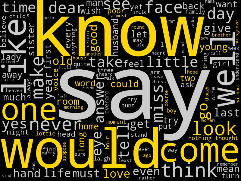
The final wordcloud we’ve created is a lot more complex than the previous ones; with a max of 6000 words (almost as many as there are unique words in Addie’s Husband), it takes a lot longer to generate, and the text is noticeably smaller. However, the end result is (in my opinion) worth the effort. Though the words themselves are now somewhat hard to read (always an issue with big wordclouds), it’s an image that expresses one of the main ideas in Addie’s Husband, using words from Addie’s Husband, and I think that’s neat.
The Wordcloud library is stuffed with extra tweakable parameters, and there’s a lot more you can do to refine things than is covered in this tutorial. However, hopefully this gives some idea of the possibilities and the code to move towards them. The module documentation has many more examples.
There are a couple of caveats with wordclouds that should always be borne in mind. As already mentioned, it’s easy to make confusing or misleading word clouds, because the focus on frequency ignores any information from the text that was contained in more than one word; «not happy» and «happy» are both going to make the word «happy» appear larger.
Even if your wordclouds manage not to be misleading, that still doesn’t make them meaningful; again, the focus on frequency ignores context and significance. Even with stopwords removed, it’s clear from the wordclouds generated in this tutorial that not all words are equally informative about what’s actually happening in Addie’s Husband. The word «say» is frequent, but would be equally so in almost any long narrative text. Arguably, the elaborate style of Victorian prose means that you’ll get more frequent-but-not-significant words than a comparable modern text, but unless you do heavy cleaning, wordclouds will always contain some functional words that get in the way a bit.
With the above said though, I still think wordclouds are a useful thing to be able to generate; as long as you bear the caveats in mind, and don’t use them too heavily as actual analysis tools, they’re an accessible and appealing visualisation that people respond to well.
You can find a complete copy of the code for this tutorial on Github, along with the text data and images used throughout.
If you create any wordclouds using this tutorial, I’d love to see them. Send them to me via the links in my author bio, or tweet them to me at @peritract.
Improve Article
Save Article
Like Article
Improve Article
Save Article
Like Article
Word Cloud is a data visualization technique used for representing text data in which the size of each word indicates its frequency or importance. Significant textual data points can be highlighted using a word cloud. Word clouds are widely used for analyzing data from social network websites.
For generating word cloud in Python, modules needed are – matplotlib, pandas and wordcloud. To install these packages, run the following commands :
pip install matplotlib
pip install pandas
pip install wordcloud
The dataset used for generating word cloud is collected from UCI Machine Learning Repository. It consists of YouTube comments on videos of popular artists.
Dataset Link : https://archive.ics.uci.edu/ml/machine-learning-databases/00380/
Below is the implementation :
Python3
from wordcloud import WordCloud, STOPWORDS
import matplotlib.pyplot as plt
import pandas as pd
df = pd.read_csv(r"Youtube04-Eminem.csv", encoding ="latin-1")
comment_words = ''
stopwords = set(STOPWORDS)
for val in df.CONTENT:
val = str(val)
tokens = val.split()
for i in range(len(tokens)):
tokens[i] = tokens[i].lower()
comment_words += " ".join(tokens)+" "
wordcloud = WordCloud(width = 800, height = 800,
background_color ='white',
stopwords = stopwords,
min_font_size = 10).generate(comment_words)
plt.figure(figsize = (8, 8), facecolor = None)
plt.imshow(wordcloud)
plt.axis("off")
plt.tight_layout(pad = 0)
plt.show()
Output :
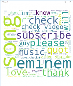
The above word cloud has been generated using Youtube04-Eminem.csv file in the dataset. One interesting task might be generating word clouds using other csv files available in the dataset.
Advantages of Word Clouds :
- Analyzing customer and employee feedback.
- Identifying new SEO keywords to target.
Drawbacks of Word Clouds :
- Word Clouds are not perfect for every situation.
- Data should be optimized for context.
Reference : https://en.wikipedia.org/wiki/Tag_cloud
Like Article
Save Article
#статьи
- 4 май 2021
-
15
Создаём простую и красивую инфографику из странички на «Википедии».

Кандидат философских наук, специалист по математическому моделированию. Пишет про Data Science, AI и программирование на Python.
В любой непонятной ситуации дата-сайентист визуализирует данные: это, среди прочего, облегчает поиск инсайтов и формулирование гипотез для проверки.
«Облако слов» — визуализация текстовых данных на стыке исследовательского анализа, инфографики и дата-дизайна. Это самый первый и быстрый взгляд на большие и слабо структурированные тексты: художественные, научные, информационные.
Главные причины использовать облако слов:
- Во-первых, это красиво — удачная визуализация украшает портфолио.
- Во-вторых, облако показывает самые популярные слова текста, что полезно для быстрой его оценки.
Например, для школьного сочинения или текста в разговорном стиле это могут оказаться слова-паразиты (от таких неплохо бы избавляться), а для научных или «инфостильных» текстов — слова, больше относящиеся к содержанию.
- В-третьих, сделать такую визуализацию совсем не сложно — и сейчас вы сами в этом убедитесь.
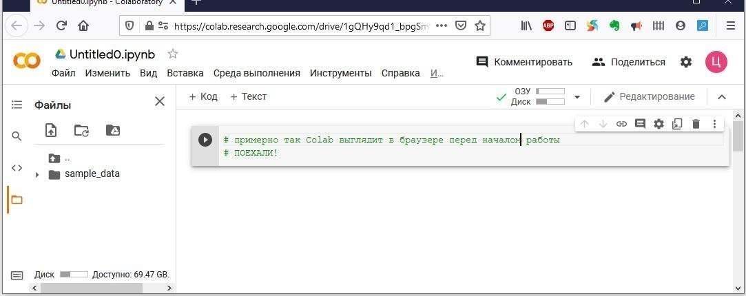
Мы будем работать в блокноте Google Colab — то есть прямо в браузере, код напишем на языке Python, а текст возьмём из «Википедии». Если что-то пойдёт не так — всегда можно свериться с нашим блокнотом: все ссылки есть в конце статьи.
Для начала работы в Colab достаточно войти в свой Gmail и запустить приветственный блокнот в браузере. Не помешает и прочитать пару наших статей: про Colab и про Python-минимум для дата-сайентиста.
После запуска колаба нужно установить библиотеку для работы с «Википедией» и библиотеку stop-words, в которой содержатся списки стоп-слов для анализа текстов на разных языках.
!pip install wikipedia
!pip install stop-words
Запустите каждую команду в отдельной кодовой ячейке: так проще отследить результат выполнения.
Сперва подготовим входной текст:
# Импортируем нужные библиотеки
import wikipedia
import re

# Выбираем язык Википедии и интересующую нас страницу
wikipedia.set_lang("ru")
wiki = wikipedia.page('Гарри Поттер')

# Извлекаем текст из полученной страницы
text = wiki.content

# Очищаем текст с помощью регулярных выражений
text = re.sub(r'==.*?==+', '', text) # удаляем лишние символы
text = text.replace('n', '') # удаляем знаки разделения на абзацы
Мы импортировали в проект только что установленную библиотеку wikipedia и библиотеку re для работы с регулярными выражениями. Затем указали язык «Википедии» и имя интересующей нас страницы (сохранили её в переменную wiki). Разумеется, вы можете взять любую другую страницу.

Текстовое содержимое страницы ушло в переменную text, после чего с помощью регулярных выражений мы удалили из него ненужные символы (знаки препинания, перевода абзацев, лишние разделители).
Теперь нам нужны библиотека и функция для визуализации текста. Библиотеку мы импортируем, а функцию напишем сами — она нам ещё пригодится.
# Импортируем библиотеку для визуализации
import matplotlib.pyplot as plt
%matplotlib inline

# Функция для визуализации облака слов
def plot_cloud(wordcloud):
    # Устанавливаем размер картинки
    plt.figure(figsize=(40, 30))
    # Показать изображение
    plt.imshow(wordcloud)
    # Без подписей на осях
    plt.axis("off")
Команда %matplotlib inline указывает, что графики будут отрисованы прямо в блокноте колаба, а не где-то в отдельном окне.
Что касается функции plot_cloud, то она принимает параметром облако слов (мы создадим его ниже), устанавливает размер картинки в дюймах и выводит её, а метод axis c аргументом «off» отключает подписи внизу и слева.
Всё почти готово, осталось главное.
# Импортируем инструменты для облака слов и списки стоп-слов
from wordcloud import WordCloud
from stop_words import get_stop_words

# Записываем в переменную стоп-слова русского языка
STOPWORDS_RU = get_stop_words('russian')

# Генерируем облако слов
wordcloud = WordCloud(width = 2000,
                      height = 1500,
                      random_state=1,
                      background_color='black',
                      margin=20,
                      colormap='Pastel1',
                      collocations=False,
                      stopwords = STOPWORDS_RU).generate(text)

# Рисуем картинку
plot_cloud(wordcloud)
Вы можете добавить свои стоп-слова в переменную STOPWORDS_RU с помощью метода .add (‘новое стоп-слово’).
Параметр random_state=1 — если не указать, то при каждом запуске функции облако слов будет отличаться от предыдущего.
Параметр collocations определяет, включать ли в итоговую картинку сочетания из двух слов (так называемые биграммы). У нас он отключён, поэтому фраз в облаке не будет.
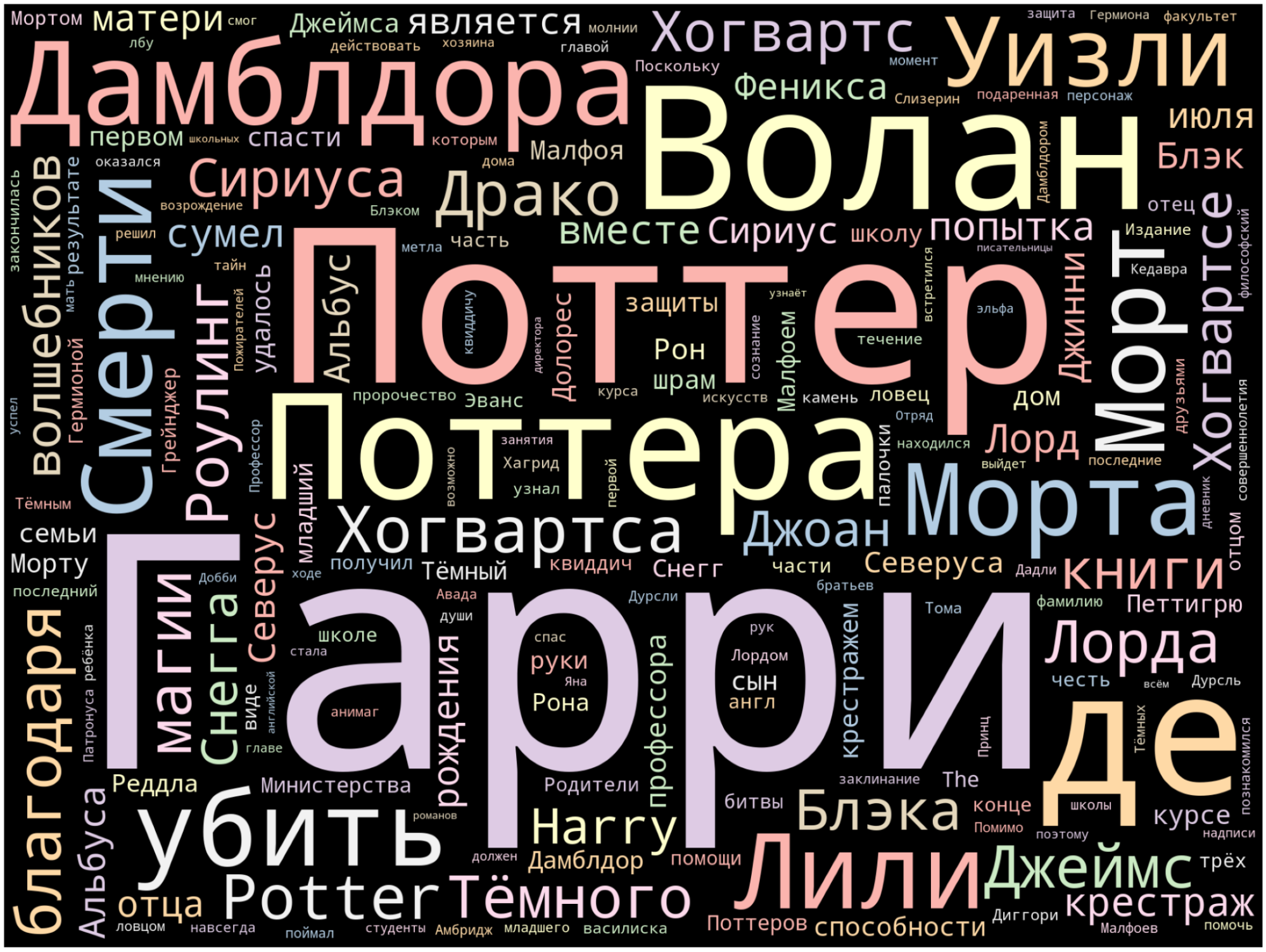
Сохраним получившуюся картинку в файл:
wordcloud.to_file('hp_cloud_simple.png')
Её можно будет найти в меню «Файлы» слева и скачать.
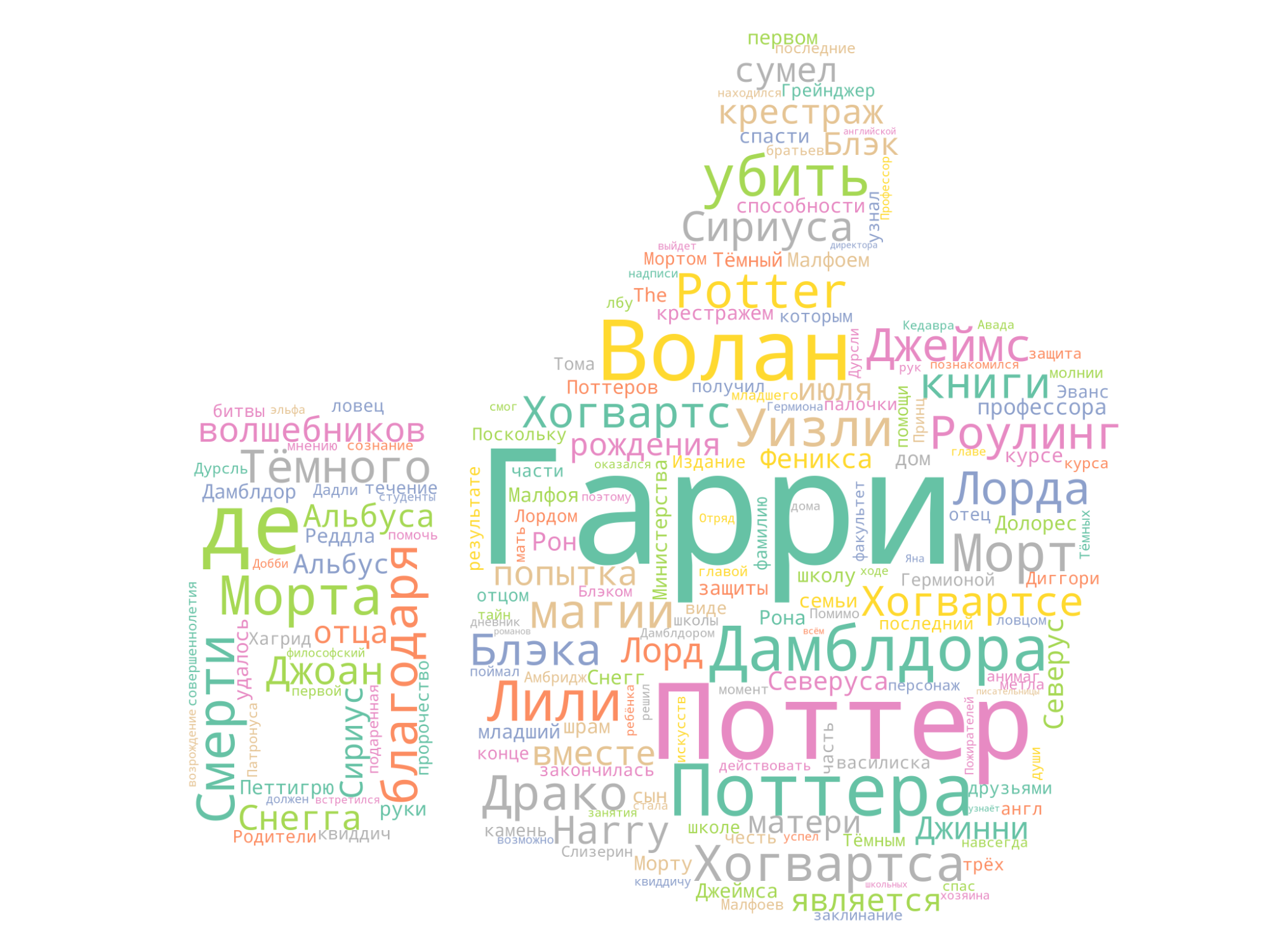
Чтобы сделать облако более замысловатой формы, чем прямоугольник, нам понадобится картинка. Она должна быть достаточно контрастной, лучше всего чёрно-белой, и без мелких деталей.
Я скачал картинку под названием upvote.png отсюда. Вы можете поступить так же. После этого перетащите её в список файлов и папок в левой части блокнота.
# Импортируем необходимое
import numpy as np
from PIL import Image

# Превращаем картинку в маску
mask = np.array(Image.open('/content/upvote.png'))

# Генерируем облако слов
wordcloud = WordCloud(width = 2000,
                      height = 1500,
                      random_state=1,
                      background_color='white',
                      colormap='Set2',
                      collocations=False,
                      stopwords = STOPWORDS_RU,
                      mask=mask).generate(text)

# Выводим его на экран
plot_cloud(wordcloud)
Импортировали библиотеку NumPy и нужную нам функцию Image из библиотеки PIL (Python Imaging Library). С их помощью мы считаем картинку из файла и превратим её в маску (переменная mask), по которой и будет отрисовываться облако слов.
Обратите внимание, что mask появилась и в параметрах функции WordCloud ().
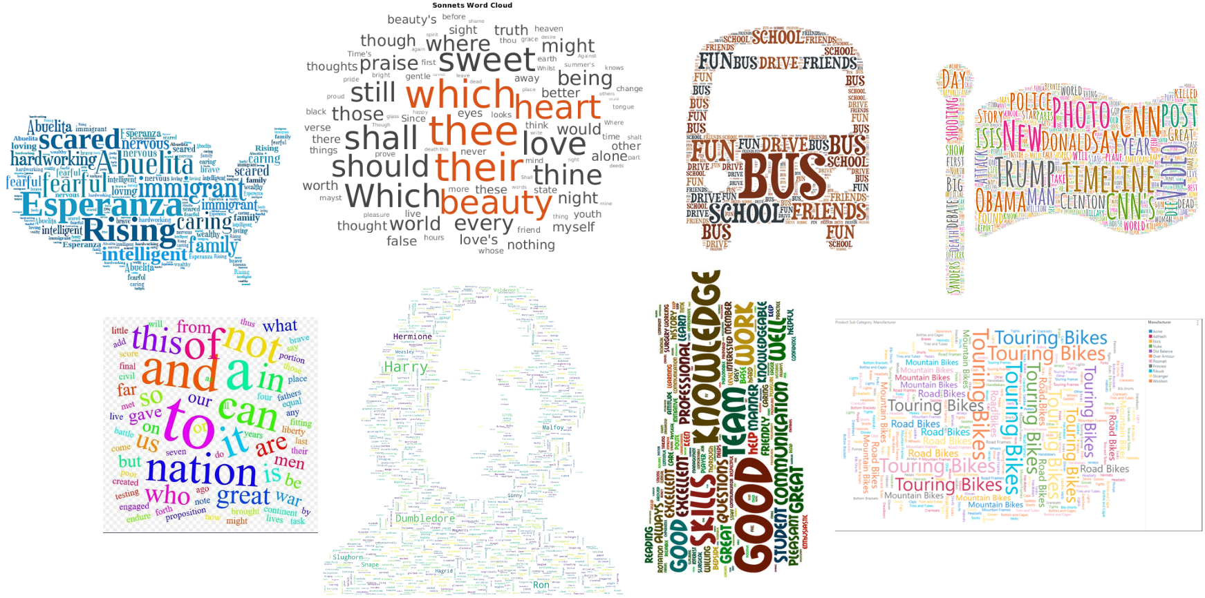
Вот что у нас вышло на этот раз:
Ссылка на наш ноутбук здесь. Скопируйте его на свой Google-диск через пункт меню «Файл» и начинайте экспериментировать: поиграйтесь с размерами и форматами картинки-маски и самого облака; выясните, как на него влияют параметры random_state, colormap и collocations.
Опирайтесь на документацию библиотеки, и да пребудут с вами Сила Питона и Дух Данных!
На курсе «Профессия Data Scientist» учат делать гораздо более продвинутые визуализации и обрабатывать самые запутанные данные. Опытные преподаватели и заряженные единомышленники ждут вас.

Научитесь: Профессия Data Scientist
Узнать больше
Время на прочтение
6 мин
Количество просмотров 48K
Частотный анализ является одним из сравнительно простых методов обработки текста на естественном языке (NLP). Его результатом является список слов, наиболее часто встречающихся в тексте. Частотный анализ также позволяет получить представление о тематике и основных понятиях текста. Визуализировать его результаты удобно в виде «облака слов». Эта диаграмма содержит слова, размер шрифта которых отражает их популярность в тексте.
Обработку текста на естественном языке удобно производить с помощью Python, поскольку он является достаточно высокоуровневым инструментом программирования, имеет развитую инфраструктуру, хорошо зарекомендовал себя в сфере анализа данных и машинного обучения. Сообществом разработано несколько библиотек и фреймворков для решения задач NLP на Python. Мы в своей работе будем использовать интерактивный веб-инструмент для разработки python-скриптов Jupyter Notebook, библиотеку NLTK для анализа текста и библиотеку wordcloud для построения облака слов.
В сети представлено достаточно большое количество материала по теме анализа текста, но во многих статьях (в том числе русскоязычных) предлагается анализировать текст на английском языке. Анализ русского текста имеет некоторую специфику применения инструментария NLP. В качестве примера рассмотрим частотный анализ текста повести «Метель» А. С. Пушкина.
Проведение частотного анализа можно условно разделить на несколько этапов:
- Загрузка и обзор данных
- Очистка и предварительная обработка текста
- Удаление стоп-слов
- Перевод слов в основную форму
- Подсчёт статистики встречаемости слов в тексте
- Визуализация популярности слов в виде облака
Скрипт доступен по адресу github.com/Metafiz/nlp-course-20/blob/master/frequency-analisys-of-text.ipynb, исходный текст — github.com/Metafiz/nlp-course-20/blob/master/pushkin-metel.txt
Загрузка данных
Открываем файл с помощью встроенной функции open, указываем режим чтения и кодировку. Читаем всё содержимое файла, в результате получаем строку text:
f = open('pushkin-metel.txt', "r", encoding="utf-8")
text = f.read()
Длину текста – количество символов – можно получить стандартной функцией len:
len(text)
Строка в python может быть представлена как список символов, поэтому для работы со строками также возможны операции доступа по индексам и получения срезов. Например, для просмотра первых 300 символов текста достаточно выполнить команду:
text[:300]
Предварительная обработка (препроцессинг) текста
Для проведения частотного анализа и определения тематики текста рекомендуется выполнить очистку текста от знаков пунктуации, лишних пробельных символов и цифр. Сделать это можно различными способами – с помощью встроенных функций работы со строками, с помощью регулярных выражений, с помощью операций обработки списков или другим способом.
Для начала переведём символы в единый регистр, например, нижний:
text = text.lower()
Используем стандартный набор символов пунктуации из модуля string:
import string
print(string.punctuation)
string.punctuation представляет собой строку. Набор специальных символов, которые будут удалены из текста может быть расширен. Необходимо проанализировать исходный текст и выявить символы, которые следует удалить. Добавим к знакам пунктуации символы переноса строки, табуляции и другие символы, которые встречаются в нашем исходном тексте (например, символ с кодом xa0):
spec_chars = string.punctuation + 'nxa0«»t—…'
Для удаления символов используем поэлементную обработку строки – разделим исходную строку text на символы, оставим только символы, не входящие в набор spec_chars и снова объединим список символов в строку:
text = "".join([ch for ch in text if ch not in spec_chars])
Можно объявить простую функцию, которая удаляет указанный набор символов из исходного текста:
def remove_chars_from_text(text, chars):
    return "".join([ch for ch in text if ch not in chars])
Её можно использовать как для удаления спец.символов, так и для удаления цифр из исходного текста:
text = remove_chars_from_text(text, spec_chars)
text = remove_chars_from_text(text, string.digits)
Токенизация текста
Для последующей обработки очищенный текст необходимо разбить на составные части – токены. В анализе текста на естественном языке применяется разбиение на символы, слова и предложения. Процесс разбиения называется токенизация. Для нашей задачи частотного анализа необходимо разбить текст на слова. Для этого можно использовать готовый метод библиотеки NLTK:
from nltk import word_tokenize
text_tokens = word_tokenize(text)
Переменная text_tokens представляет собой список слов (токенов). Для вычисления количества слов в предобработанном тексте можно получить длину списка токенов:
len(text_tokens)
Для вывода первых 10 слов воспользуемся операцией среза:
text_tokens[:10]
Для применения инструментов частотного анализа библиотеки NLTK необходимо список токенов преобразовать к классу Text, который входит в эту библиотеку:
import nltk
text = nltk.Text(text_tokens)
Выведем тип переменной text:
print(type(text))
К переменной этого типа также применимы операции среза. Например, это действие выведет 10 первых токенов из текста:
text[:10]
Подсчёт статистики встречаемости слов в тексте
Для подсчёта статистики распределения частот слов в тексте применяется класс FreqDist (frequency distributions):
from nltk.probability import FreqDist
fdist = FreqDist(text)
Попытка вывести переменную fdist отобразит словарь, содержащий токены и их частоты – количество раз, которые эти слова встречаются в тексте:
FreqDist({'и': 146, 'в': 101, 'не': 69, 'что': 54, 'с': 44, 'он': 42, 'она': 39, 'ее': 39, 'на': 31, 'было': 27, ...})
Также можно воспользоваться методом most_common для получения списка кортежей с наиболее часто встречающимися токенами:
fdist.most_common(5)

[('и', 146), ('в', 101), ('не', 69), ('что', 54), ('с', 44)]
Частота распределения слов тексте может быть визуализирована с помощью графика. Класс FreqDist содержит встроенный метод plot для построения такого графика. Необходимо указать количество токенов, частоты которых будут показаны на графике. С параметром cumulative=False график иллюстрирует закон Ципфа: если все слова достаточно длинного текста упорядочить по убыванию частоты их использования, то частота n-го слова в таком списке окажется приблизительно обратно пропорциональной его порядковому номеру n.
fdist.plot(30,cumulative=False)
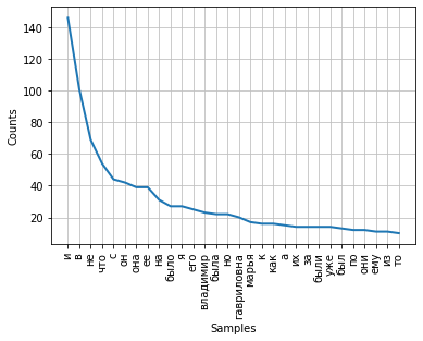
Можно заметить, что в данный момент наибольшие частоты имеют союзы, предлоги и другие служебные части речи, не несущие смысловой нагрузки, а только выражающие семантико-синтаксические отношения между словами. Для того, чтобы результаты частотного анализа отражали тематику текста, необходимо удалить эти слова из текста.
Удаление стоп-слов
К стоп-словам (или шумовым словам), как правило, относят предлоги, союзы, междометия, частицы и другие части речи, которые часто встречаются в тексте, являются служебными и не несут смысловой нагрузки – являются избыточными.
Библиотека NLTK содержит готовые списки стоп-слов для различных языков. Получим список сто-слов для русского языка:
from nltk.corpus import stopwords
russian_stopwords = stopwords.words("russian")
Следует отметить, что стоп-слова являются контекстно зависимыми – для текстов различной тематики стоп-слова могут отличаться. Как и в случае со спец.символами, необходимо проанализировать исходный текст и выявить стоп-слова, которые не вошли в типовой набор.
Список стоп-слов может быть расширен с помощью стандартного метода extend:
russian_stopwords.extend(['это', 'нею'])
После удаления стоп-слов частота распределения токенов в тексте выглядит следующим образом:
fdist_sw.most_common(10)

[('владимир', 23),
 ('гавриловна', 20),
 ('марья', 17),
 ('поехал', 9),
 ('бурмин', 9),
 ('поминутно', 8),
 ('метель', 7),
 ('несколько', 6),
 ('сани', 6),
 ('владимира', 6)]
Как видно, результаты частотного анализа стали более информативными и точнее стали отражать основную тематику текста. Однако, мы видим в результатах такие токены, как «владимир» и «владимира», которые являются, по сути, одним словом, но в разных формах. Для исправления этой ситуации необходимо слова исходного текста привести к их основам или изначальной форме – провести стемминг или лемматизацию.
Визуализация популярности слов в виде облака
В завершение нашей работы визуализируем результаты частотного анализа текста в виде «облака слов».
Для этого нам потребуются библиотеки wordcloud и matplotlib:
from wordcloud import WordCloud
import matplotlib.pyplot as plt
%matplotlib inline
Для построения облака слов на вход методу необходимо передать строку. Для преобразования списка токенов после предобработки и удаления стоп-слов воспользуемся методом join, указав в качестве разделителя пробел:
text_raw = " ".join(text)
Выполним вызов метода построения облака:
wordcloud = WordCloud().generate(text_raw)
В результате получаем такое «облако слов» для нашего текста:

Глядя на него, можно получить общее представление о тематике и главных персонажах произведения.