
Introduction
Statistical laws describing the properties of word use, such as Zipf ‘s law1,2,3,4,5,6 and Heaps’ law7,8, have been thoroughly tested and modeled. These statistical laws are based on static snapshots of written language using empirical data aggregated over relatively small time periods and comprised of relatively small corpora ranging in size from individual texts1,2 to relatively small collections of topical texts3,4. However, language is a fundamentally dynamic complex system, consisting of heterogenous entities at the level of the units (words) and the interacting users (us). Hence, we begin this paper with two questions: (i) Do languages exhibit dynamical patterns? (ii) Do individual words exhibit dynamical patterns?
The coevolutionary nature of language requires analysis both at the macro and micro scale. Here we apply interdisciplinary concepts to empirical language data collected in a massive book digitization effort by Google Inc., which recently unveiled a database of words in seven languages, after having scanned approximately 4% of the world’s books. The massive “n-gram” project9 allows for a novel view into the growth dynamics of word use and the birth and death processes of words in accordance with evolutionary selection laws10.
A recent analysis of this database by Michel et al.11 addresses numerous well-posed questions rooted in cultural anthropology using case studies of individual words. Here we take an alternative approach by analyzing the aggregate properties of the language dynamics recorded in the Google Inc. data in a systematic way, using the word counts of every word recorded over the 209-year time period 1800 – 2008 in the English, Spanish and Hebrew text corpora. This period spans the incredibly rich cultural history that includes several international wars, revolutions and numerous technological paradigm shifts. Together, the data comprise over 1 × 10⁷ distinct words. We use concepts from economics to gain quantitative insights into the role of exogenous factors on the evolution of language, combined with methods from statistical physics to quantify the competition arising from correlations between words12,13,14 and the memory-driven autocorrelations in ui(t) across time15,16,17.
For each corpora comprising millions of distinct words, we use a general word-count framework which accounts for the underlying growth of language over time. We first define the quantity ui(t) as the number of uses of word i in year t. Since the number of books and the number of distinct words have grown dramatically over time, we define the relative word use, fi(t), as the fraction of uses of word i out of all word uses in the same year,

where the quantity  is the total number of indistinct word uses digitized from books printed in year t and Nw(t) is the total number of distinct words digitized from books printed in year t. To quantify the dynamic properties of word prevalence at the micro scale and their relation to socio-political factors at the macro scale, we analyze the logarithmic growth rate commonly used in finance and economics,

Here we analyze the single year growth rates, Δt≡1.
The relative use fi(t) depends on the intrinsic grammatical utility of the word (related to the number of “proper” sentences that can be constructed using the word), the semantic utility of the word (related to the number of meanings a given word can convey) and other idiosyncratic details related to topical context. Neutral null models for the evolution of language define the relative use of a word as its “fitness”18. In such models, the word frequency is the only factor determining the survival capacity of a word. In reality, word competition depends on more subtle features of language, such as the cognitive aspects of efficient communication. For example, the emergence of robust categorical naming patterns observed across many cultures is regarded to be the result of complex discrimination tactics shared by intelligent communicators. This is evident in the finite set of words describing the continuous spectrum of color names, emotional states and other categorical sets19,20,21.
In our analysis we treat words with equivalent meanings but with different spellings (e.g. color versus colour) as distinct words, since we view the competition among synonyms and alternative spellings in the linguistic arena as a key ingredient in complex evolutionary dynamics10,22. For instance, with the advent of automatic spell-checkers in the digital era, words recognized by spell-checkers receive a significant boost in their “reproductive fitness” at the expense of their misspelled or unstandardized counterparts.
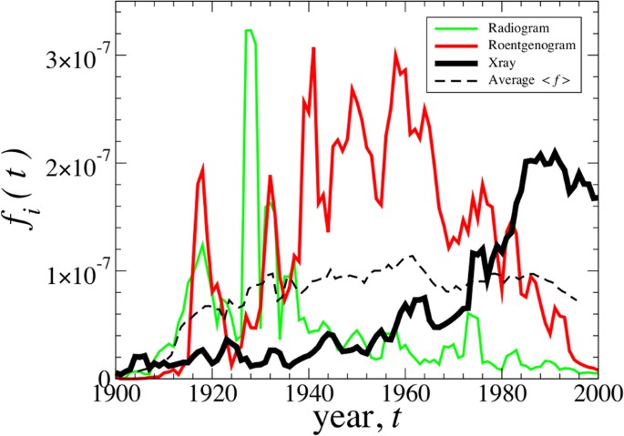
In the linguistic arena, not just “defective” words die, even significantly used words can become extinct. Fig. 1 shows three once-significant words: “Radiogram,” “Roentgenogram,” and “Xray”. These words compete for the majority share of nouns referring to what is now commonly known as an “X-ray” (note that such dashes are discarded in Google’s digitization process). The word “Roentgenogram” has since become extinct, even though it was the most common term for several decades in the 20th century. It is likely that two main factors – (i) communication and information efficiency bias toward the use of shorter words23 and (ii) the adoption of English as the leading global language for science – secured the eventual success of the word “Xray” by the year 1980. It goes without saying that there are many social and technological factors driving language change.
Word extinction.
The English word “Roentgenogram” derives from the Nobel prize winning scientist and discoverer of the X-ray, Wilhelm Röntgen (1845–1923). The prevalence of this word was quickly challenged by two main competitors, “X-ray” (recorded as “Xray” in the database) and “Radiogram.” The arithmetic mean frequency of these three time series is relatively constant over the 80-year period 1920–2000, 〈 f 〉 ≈ 10–7, illustrating the limited linguistic “market share” that can be achieved by any competitor. We conjecture that the main reason “Xray” has a higher frequency is due to the “fitness gain” from its efficient short word length and also due to the fact that English has become the base language for scientific publication.
Full size image
We begin this paper by analyzing the vocabulary growth of each language over time. We then analyze the lifetime growth trajectories of the set of words that are new to each language to gain quantitative insight into “infant” and “adult” stages of individual words. Using two sets of words, (i) the relatively new words and (ii) the most common words, we analyze the statistical properties of word growth. Specifically, we calculate the probability density function P(r) of growth rate r and calculate the size-dependence of the standard deviation σ(r) of growth rates. In order to gain insight into the long-term cultural memory, we conclude the analysis by measuring the autocorrelations in word use by applying detrended fluctuation analysis (DFA) to individual fi(t).
Results
Quantifying the birth rate and the death rate of words
Just as a new species can be born into an environment, a word can emerge in a language. Evolutionary selection laws can apply pressure on the sustainability of new words since there are limited resources (topics, books, etc.) for the use of words. Along the same lines, old words can be driven to extinction when cultural and technological factors limit the use of a word, in analogy to the environmental factors that can change the survival capacity of a living species by altering its ability to survive and reproduce.
We define the birth year y0,i as the year t corresponding to the first instance of  , where
  is median word use
  of a given word over its recorded lifetime in the Google database. Similarly, we define the death year yf,i as the last year t during which the word use satisfies
  . We use the relative word use threshold
  in order to avoid anomalies arising from extreme fluctuations in fi(t) over the lifetime of the word. The results obtained using threshold
  did not show a significant qualitative difference.
The significance of word births Δb(t) and word deaths Δd(t) for each year t is related to the vocabulary size Nw(t) of a given language. We define the birth rate γb and death rate γd by normalizing the number of births Δb(t) and deaths Δd(t) in a given year t to the total number of distinct words Nw(t) recorded in the same year t, so that
This definition yields a proxy for the rate of emergence and disappearance of words. We restrict our analysis to words with birth-death duration yf,i − y0,i + 1 ≥ 2 years and to words with first recorded use t0,i ≥ 1700, which selects for relatively new words in the history of a language.
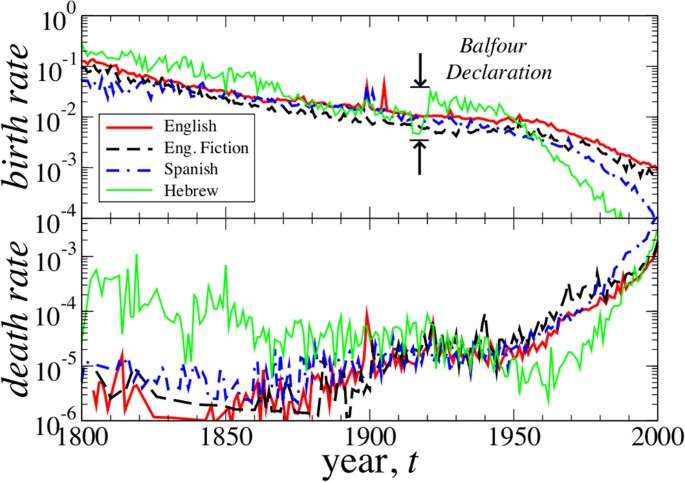
The γb(t) and γd(t) time series plotted in Fig. 2 for the 200-year period 1800–2000 show trends that intensifies after the 1950s. The modern era of publishing, which is characterized by more strict editing procedures at publishing houses, computerized word editing and automatic spell-checking technology, shows a drastic increase in the death rate of words. Using visual inspection we verify most changes to the vocabulary in the last 10–20 years are due to the extinction of misspelled words and nonsensical print errors and to the decreased birth rate of new misspelled variations and genuinely new words. This phenomenon reflects the decreasing marginal need for new words, consistent with the sub-linear Heaps’ law observed for all Google 1-gram corpora in24. Moreover, Fig. 3 shows that γb(t) is largely comprised of words with relatively large f while γd(t) is almost entirely comprised of words with relatively small f (see also Fig. S1 in the Supplementary Information (SI) text). Thus, the new words of tomorrow are likely be core words that are widely used.
Dramatic shift in the birth rate and death rate of words.
The word birth rate γb(t) and the word death rate γd(t) show marked underlying changes in word use competition which affects the entry rate and the sustainability of existing words. The modern print era shows a marked increase in the death rate of words which likely correspond to low fitness, misspelled and (technologically) outdated words. A simultaneous decrease in the birth rate of new words is consistent with the decreasing marginal need for new words indicated by the sub-linear allometric scaling between vocabulary size and total corpus size (Heaps’ law)24. Interestingly, we quantitatively observe the impact of the Balfour Declaration in 1917, the circumstances surrounding which effectively rejuvenated Hebrew as a national language, resulting in a 5-fold increase in the birth rate of words in the Hebrew corpus.
Full size image
Survival of the fittest in the entry process of words.
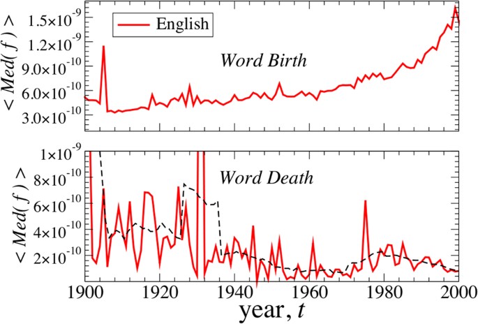
Trends in the relative uses of words that either were born or died in a given year show that the entry-exit forces largely depend on the relative use of the word. For the English corpus, we calculate the average of the median lifetime relative use, 〈Med(fi)〉, for all words born in year t (top panel) and for all words that died in year t (bottom panel), which shows a 5-year moving average (dashed black line). There is a dramatic increase in the relative use (“utility”) of newborn words over the last 20–30 years, likely corresponding to new technical terms, which are necessary for the communication of core modern technology and ideas. Conversely, with higher editorial standards and the recent use of word processors which include spelling standardization technology, the words that are dying are those words with low relative use. We confirm by visual inspection that the lists of dying words contain mostly misspelled and nonsensical words.
Full size image
We note that the main source of error in the calculation of birth and death rates are OCR (optical character recognition) errors in the digitization process, which could be responsible for a significant fraction of misspelled and nonsensical words existing in the data. An additional source of error is the variety of orthographic properties of language that can make very subtle variations of words, for example through the use of hyphens and capitalization, appear as distinct words when applying OCR. The digitization of many books in the computer era does not require OCR transfer, since the manuscripts are themselves digital and so there may be a bias resulting from this recent paradigm shift. We confirm that the statistical patterns found using post 2000- data are consistent with the patterns that extend back several hundred years24.
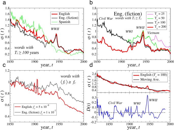
Complementary to the death of old words is the birth of new words, which are commonly associated with new social and technological trends. Topical words in media can display long-term persistence patterns analogous to earthquake shocks25,26 and can result in a new word having larger fitness than related “out-of-date” words (e.g. blog vs. log, email vs. memo). Here we show that a comparison of the growth dynamics between different languages can also illustrate the local cultural factors that influence different regions of the world. Fig. 4 shows how international crisis can lead to globalization of language through common media attention and increased lexical diffusion. Notably, as illustrated in Fig. 4(a), we find that international conflict only perturbed the participating languages, while minimally affecting the languages of the nonparticipating regions, e.g. the Spanish speaking countries during WWII.
The significance of historical events on the evolution of language.
The standard deviation σ(t) of growth rates demonstrates the sensitivity of language to international events (e.g. World War II). For all languages there is an overall decreasing trend in σ(t) over the period 1850–2000. However, the increase in σ(t) during WWII represents a“globalization” effect, whereby societies are brought together by a common event and a unified media. Such contact between relatively isolated systems necessarily leads to information flow, much as in the case of thermodynamic heat flow between two systems, initially at different temperatures, which are then brought into contact. (a) σ(t) calculated for the relatively new words with Ti ≥ 100 years. The Spanish corpus does not show an increase in σ(t) during World War II, indicative of the relative isolation of South America and Spain from the European conflict. (b) σ(t) for 4 sets of relatively new words that meet the criteria Ti ≥ Tc and ti,0 ≥ 1800. The oldest “new” words (Tc = 200) demonstrate the most significant increase in σ(t) during World War II, with a peak around 1945. (c) The standard deviation σ(t) for the most common words is decreasing with time, suggesting that they have saturated and are being “crowded out” by new competitors. This set of words meets the criterion that the average relative use exceeds a threshold, 〈fi〉 ≥ fc, which we define for each corpus. (d) We compare the variation σ(t) for relatively new English words, using Ti ≥ 100, with the 20-year moving average over the time period 1820–1988. The deviations show that σ(t) increases abruptly during times of conflict, such as the American CivilWar (1861–1865), World War I (1914–1918) and World War II (1939–1945) and also during the 1980s and 1990s, possibly as a result of new digital media (e.g. the internet) which offer new environments for the evolutionary dynamics of word use. D(t) is the difference between the moving average and σ(t).
Full size image
The lifetime trajectory of words
Between birth and death, one contends with the interesting question of how the use of words evolve when they are “alive.” We focus our efforts toward quantifying the relative change in word use over time, both over the word lifetime and throughout the course of history. In order to analyze separately these two time frames, we select two sets of words: (i) relatively new words with “birth year” t0,i later than 1800, so that the relative age τ ≡ t − t0,i of word i is the number of years after the word’s first occurrence in the database and (ii) relatively common words, typically with t0,i < 1800.
We analyze dataset (i) words (summary statistics in Table S1) so that we can control for properties of the growth dynamics that are related to the various stages of a word’s life trajectory (e.g. an “infant” phase, an “adolescent” phase and a “mature” phase). For comparison with the young words, we also analyze the growth rates of dataset (ii) words in the next section (summary statistics in Table S2). These words are presumably old enough that they are in a stable mature phase. We select dataset (ii) words using the criterion 〈fi〉 ≥ fc, where  is the average relative use of the word i over the word’s lifetime Ti = t0,f − t0,i + 1 and fc is a cutoff threshold derived form the Zipf rank-frequency distribution1 calculated for each corpus24. In Table S3 we summarize the entire data for the 209-year period 1800–2008 for each of the four Google language sets analyzed.
Modern words typically are born in relation to technological or cultural events, e.g. “Antibiotics.” We ask if there exists a characteristic time for a word’s general acceptance. In order to search for patterns in the growth rates as a function of relative word age, for each new word i at its age τ , we analyze the “use trajectory” fi(τ) and the “growth rate trajectory” ri(τ). So that we may combine the individual trajectories of words of varying prevalence, we normalize each fi(τ) by its average 〈fi〉, obtaining a normalized use trajectory  . We perform an analogous normalization procedure for each ri(τ), normalizing instead by the growth rate standard deviation σ[ri], so that
  (see the Methods section for further detailed description).
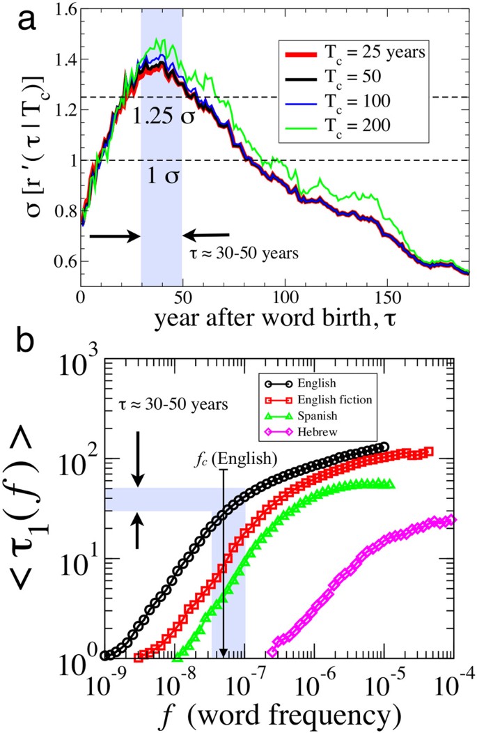
Since some words will die and other words will increase in use as a result of the standardization of language, we hypothesize that the average growth rate trajectory will show large fluctuations around the time scale for the transition of a word into regular use. In order to quantify this transition time scale, we create a subset {i |Tc} of word trajectories i by combining words that meets an age criteria Ti ≥ Tc. Thus, Tc is a threshold to distinguish words that were born in different historical eras and which have varying longevity. For the values Tc = 25, 50, 100 and 200 years, we select all words that have a lifetime longer than Tc and calculate the average and standard deviation for each set of growth rate trajectories as a function of word age τ.
In Fig. 5 we plot  for the English corpus, which shows a broad peak around τc ≈ 30–50 years for each Tc subset before the fluctuations saturate after the word enters a stable growth phase. A similar peak is observed for each corpus analyzed (Figs. S4–S7). This single-peak growth trajectory is consistent with theoretical models for logistic spreading and the fixation of words in a population of learners27. Also, since we weight the average according to 〈fi〉, the time scale τc is likely associated with the characteristic time for a new word to reach sufficiently wide acceptance that the word is included in a typical dictionary. We note that this time scale is close to the generational time scale for humans, corroborating evidence that languages require only one generation to drastically evolve27.
Quantifying the tipping point for word use.
(a) The maximum in the standard deviation σ of growth rates during the “adolescent” period τ ≈ 30–50 indicates the characteristic time scale for words being incorporated into the standard lexicon, i.e. inclusion in popular dictionaries. In Fig. S4 we plot the average growth rate trajectory 〈r′(τ|Tc)〉 which shows relatively large positive growth rates during approximately the same 20-year period. (b) The first passage time τ153 is defined as the number years for the relative use of a new word i to exceed a given f-value for the first time, fi(τ1) ≥ f. For relatively new words with Ti ≥ 100 years we calculate the average first-passage time 〈τ1(f)〉 for a large range of f. We estimate for each language the fc representing the threshold for a word belonging to the standard “kernel” lexicon4. This method demonstrates that the English corpus threshold fc ≡ 5 × 10⁻⁸ maps to the first passage time corresponding to the peak period τ ≈ 30 – 50 years in σ(τ) shown in panel (a).
Full size image
Empirical laws quantifying the growth rate distribution
How much do the growth rates vary from word to word? The answer to this question can help distinguish between candidate models for the evolution of word utility. Hence, we calculate the probability density function (pdf) of  . Using this quantity accounts for the fact that we are aggregating growth rates of words of varying ages. The empirical pdf P(R) shown in Fig. 6 is leptokurtic and remarkably symmetric around R ≈ 0. These empirical facts are also observed in studies of the growth rates of economic institutions28,29,30,31. Since the R values are normalized and detrended according to the age-dependent standard deviation σ[r′(τ|Tc)], the standard deviation is σ(R) = 1 by construction.
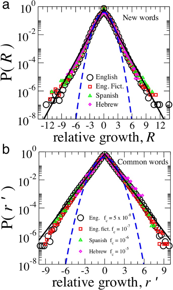
Common leptokurtic growth distribution for new words and common words.
(a) Independent of language, the growth rates of relatively new words are distributed according to the Laplace distribution centered around R ≈ 0 defined in Eq. (4). The the growth rate R defined in Eq. (11) is measured in units of standard deviation and accounts for age-dependent and word-dependent factors. Yet, even with these normalizations, we still observe an excess number of |R| ≥ 3σ events. This fact is demonstrated by the leptokurtic form of each P(R), which exhibit the excess tail frequencies when compared with a unit-variance Gaussian distribution (dashed blue curve). The Gaussian distribution is the predicted distribution for the Gibrat proportional growth model, which is a candidate neutral null-model for the growth dynamics of word use29. The prevalence of large growth rates illustrate the possibility that words can have large variations in use even over the course of a year. The growth variations are intrinsically related to the dynamics of everyday life and reflect the cultural and technological shocks in society. We analyze word use data over the time period 1800–2008 for new words i with lifetimes Ti ≥ Tc, where we show data calculated for Tc = 100 years. (b) PDF P(r′) of the annual relative growth rate r′ for all words which satisfy 〈fi〉 ≥ fc (dataset #ii words which are relatively common words). In order to select relatively frequently used words, we use the following criteria: Ti ≥ 10 years, 1800 ≤ t ≤ 2008 and 〈fi〉 ≥ fc. The growth rate r′ does not account for age-dependent factors since the common words are likely in the mature phase of their lifetime trajectory. In each panel, we plot a Laplace distribution with unit variance (solid black lines) and the Gaussian distribution with unit variance (dashed blue curve) for reference.
Full size image
A candidate model for the growth rates of word use is the Gibrat proportional growth process29,30, which predicts a Gaussian distribution for P(R). However, we observe the “tent-shaped” pdf P(R) which is well-approximated by a Laplace (double-exponential) distribution, defined as
Here the average growth rate 〈R〉 has two properties: (a) 〈R〉 ≈ 0 and (b) 〈R〉 ≪ σ(R). Property (a) arises from the fact that the growth rate of distinct words is quite small on the annual basis (the growth rate of books in the Google English database is γw ≈ 0.01124) and property (b) arises from the fact that R is defined in units of standard deviation. Being leptokurtic, the Laplace distribution predicts an excess number of events > 3σ as compared to the Gaussian distribution. For example, comparing the likelihood of events above the 3σ event threshold, the Laplace distribution displays a five-fold excess in the probability P(|R − 〈R〉| > 3σ), where  for the Laplace distribution, whereas
  for the Gaussian distribution. The large R values correspond to periods of rapid growth and decline in the use of words during the crucial “infant” and “adolescent” lifetime phases. In Fig. 6(b) we also show that the growth rate distribution P(r′) for the relatively common words comprising dataset (ii) is also well-described by the Laplace distribution.
For hierarchical systems consisting of units each with complex internal structure32 (e.g. a given country consists of industries, each of which consists of companies, each of which consists of internal subunits), a non-trivial scaling relation between the standard deviation of growth rates σ(r|S) and the system size S has the form

The theoretical prediction in32,33 that β ∈ [0, 1/2] has been verified for several economic systems, with empirical β values typically in the range 0.1 < β < 0.333.
Since different words have varying lifetime trajectories as well as varying relative utilities, we now quantify how the standard deviation σ(r|Si) of growth rates r depends on the cumulative word frequency

of each word. We choose this definition for proxy of “word size” since a writer can learn and recall a given word through any of its historical uses. Hence, Si is also proportional to the number of books in which word i appears. This is significantly different than the assumptions of replication null models (e.g. the Moran process) which use the concurrent frequency fi(t) as the sole factor determining the likelihood of future replication10,18.
We estimate Eq. (5) by grouping words according to Si and then calculating the growth rate standard deviation σ(r|Si) for each group. Fig. 7(b) shows scaling behavior consistent with Eq. (5) for large Si, with β ≈ 0.10 – 0.21 depending on the corpus. A positive β value means that words with larger cumulative word frequency have smaller annual growth rate fluctuations. We conjecture that this statistical pattern emerges from the hierarchical organization of written language12,13,14,15,16 and the social properties of the speakers who use the words8,17,34. As such, we calculate β values that are consistent with nontrivial correlations in word use, likely related to the basic fact that books are topical3 and that book topics are correlated with cultural trends.
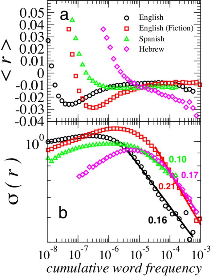
Scaling in the growth rate fluctuations of words.
We show the dependence of growth rates on the cumulative word frequency  using words satisfy the criteria Ti ≥ 10 years. We verify similar results for threshold values Tc = 50, 100 and 200 years. (a) Average growth rate 〈r〉 saturates at relatively constant values for large S. (b) Scaling in the standard deviation of growth rates σ(r|S) ∼ S–β for words with large S. This scaling relation is also observed for the growth rates of large economic institutions, ranging in size from companies to entire countries31,33. Here this size-variance relation corresponds to scaling exponent values 0.10 < β < 0.21, which are related to the non-trivial bursting patterns and non-trivial correlation patterns in literature topicality as indicated by the quantitative relation to the Hurst exponent, H = 1 – β shown in35. We calculate βEng. ≈ 0.16 ± 0.01, βEng.fict ≈ 0.21 ± 0.01, βSpa. ≈ 0.10 ± 0.01 and βHeb. ≈ 0.17 ± 0.01.
Full size image
Quantifying the long-term cultural memory
Recent theoretical work35 shows that there is a fundamental relation between the size-variance exponent β and the Hurst exponent H quantifying the auto-correlations in a stochastic time series. The novel relation H = 1 − β indicates that the temporal long-term persistence is intrinsically related to the capability of the underlying mechanism to absorb stochastic shocks. Hence, positive correlations (H > 1/2) are predicted for non-trivial β values (i.e. 0 ≤ β ≤ 0.5). Note that the Gibrat proportional growth model predicts β = 0 and that a Yule-Simon urn model predicts β = 0.533. Thus, fi(τ) belonging to words with large Si are predicted to show significant positive correlations, Hi > 1/2.
To test this connection between memory correlations and the size-variance scaling, we calculate the Hurst exponent Hi for each time series belonging to the more relatively common words analyzed in dataset (ii) using detrended fluctuation analysis (DFA)35,36,37. We plot in Fig. S2 the relative use time series fi(t) for the words “polyphony,” “Americanism,” “Repatriation,” and “Antibiotics” along with DFA curves from which we calculate each Hi. Fig. S2(b) shows that the Hi values for these four words are all significantly greater than Hr = 0.5, which is the expected Hurst exponent for a stochastic time series with no temporal correlations. In Fig. S3 we plot the distribution of Hi values for the English fiction corpus and the Spanish corpus. Our results are consistent with the theoretical prediction 〈H〉 = 1 − β established in35 relating the variance of growth rates to the underlying temporal correlations in each fi(t). Hence, we show that the language evolution is fundamentally related to the complex features of cultural memory, i.e. the dynamics of cultural topic formation17,25,26,34 and bursting38,39.
Discussion
With the digitization of written language, cultural trend analysis based around methods to extract quantitative patterns from word counts is an emerging interdisciplinary field that has the potential to provide novel insights into human sociology3,17,25,26,34,40. Nevertheless, the amount of metadata extractable from daily internet feeds is dizzying. This is highlighted by the practical issue of defining objective significance levels to filter out the noise in the data deluge. For example, online blogs can be vaguely categorized according to the coarse hierarchical schema: “obscure blogs”, “more popular blogs”, “pop columns” and “mainstream news coverage.” In contrast, there are well-defined entry requirements for published books and magazines, which must meet editorial standards and conform to the principles of market supply and demand. However, until recently, the vast information captured in the annals of written language was largely inaccessible.
Despite the careful guard of libraries around the world, which house the written corpora for almost every written language, little is known about the aggregate dynamics of word evolution in written history. Inspired by research on the growth patterns displayed by a wide range of competition driven systems — from countries and business firms28,29,30,31,32,33,41,42,43,44 to religious activities45, universities46, scientific journals47, careers48 and bird populations49 — here we extend the concepts and methods to word use dynamics.
This study provides empirical evidence that words are competing actors in a system of finite resources. Just as business firms compete for market share, words demonstrate the same growth statistics because they are competing for the use of the writer/speaker and for the attention of the corresponding reader/listener18,19,20,21,27. A prime example of fitness-mediated evolutionary competition is the case of irregular and regular verb use in English. By analyzing the regularization rate of irregular verbs through the history of the English language, Lieberman et al.50 show that the irregular verbs that are used more frequently are less likely to be overcome by their regular verb counterparts. Specifically, they find that the irregular verb death rate scales as the inverse square root of the word’s relative use. A study of word diffusion across Indo-European languages shows similar frequency-dependence of word replacement rates51.
We document the case example of X-ray, which shows how categorically related words can compete in a zero-sum game. Moreover, this competition does not occur in a vacuum. Instead, the dynamics are significantly related to diffusion and technology. Lexical diffusion occurs at many scales, both within relatively small groups and across nations27,34,51. The technological forces underlying word selection have changed significantly over the last 20 years. With the advent of automatic spell-checkers in the digital era, words recognized by spell-checkers receive a significant boost in their “reproductive fitness” at the expense of their “misspelled” or unstandardized counterparts.
We find that the dynamics are influenced by historical context, trends in global communication and the means for standardizing that communication. Analogous to recessions and booms in a global economy, the marketplace for words waxes and wanes with a global pulse as historical events unfold. And in analogy to financial regulations meant to limit risk and market domination, standardization technologies such as the dictionary and spell checkers serve as powerful arbiters in determining the characteristic properties of word evolution. Context matters and so we anticipate that niches34 in various language ecosystems (ranging from spoken word to professionally published documents to various online forms such as chats, tweets and blogs) have heterogenous selection laws that may favor a given word in one arena but not another. Moreover, the birth and death rate of words and their close associates (misspellings, synonyms, abbreviations) depend on factors endogenous to the language domain such as correlations in word use to other partner words and polysemous contexts12,13 as well as exogenous socio-technological factors and demographic aspects of the writers, such as age13 and social niche34.
We find a pronounced peak in the fluctuations of word growth rates when a word has reached approximately 30–50 years of age (see Fig. 5). We posit that this corresponds to the timescale for a word to be accepted into a standardized dictionary which inducts words that are used above a threshold frequency, consistent with the first-passage times to fc in Fig. 5(b). This is further corroborated by the characteristic baseline frequencies associated with standardized dictionaries11. Another important timescale in evolutionary systems is the reproduction age of the interacting gene or meme host. Interestingly, a 30–50 year timescale is roughly equal to the characteristic human generational time scale. The prominent role of new generation of speakers in language evolution has precedent in linguistics. For example, it has been shown that primitive pidgin languages, which are little more than crude mixes of parent languages, spontaneously acquire the full range of complex syntax and grammar once they are learned by the children of a community as a native language. It is at this point a pidgin becomes a creole, in a process referred to as nativization22.
Nativization also had a prominent effect in the revival of the Hebrew language, a significant historical event which also manifests prominently in our statistical analysis. The birth rate of new words in the Hebrew language jumped by a factor of 5 in just a few short years around 1920 following the Balfour Declaration of 1917 and the Second Aliyah immigration to Israel. The combination of new Hebrew-speaking communities and political endorsement of a national homeland for the Jewish people in the Palestine Mandate had two resounding affects: (i) the Hebrew language, hitherto used largely only for (religious) writing, gained official status as a modern spoken language and (ii) a centralized culture emerged from this national community. The unique history of the Hebrew language in concert with the Google Inc. books data thus provide an unprecedented opportunity to quantitatively study the emerging dynamics of what is, in some regards, a new language.
The impact of historical context on language dynamics is not limited to emerging languages, but extends to languages that have been active and evolving continuously for a thousand years. We find that historical episodes can drastically perturb the properties of existing languages over large time scales. Moreover, recent studies show evidence for short-timescale cascading behavior in blog trends25,26, analogous to the aftershocks following earthquakes and the cascades of market volatility following financial news announcements52. The nontrivial autocorrelations and the leptokurtic growth distributions demonstrate the significance of exogenous shocks which can result in growth rates that significantly exceeding the frequencies that one would expect from non-interacting proportional growth models29,30.
A large number of the world’s ethnic groups are separated along linguistic lines. A language barrier can isolate its speakers by serving as a screen to external events, which may further slow the rate of language evolution by stalling endogenous change. Nevertheless, we find that the distribution of word growth rates significantly broadens during times of large scale conflict, revealed through the sudden increases in σ(t) for the English, French, German and Russian corpora during World War II24. This can be understood as manifesting from the unification of public consciousness that creates fertile breeding ground for new topics and ideas. During war, people may be more likely to have their attention drawn to global issues. Remarkably, the pronounced change during WWII was not observed for the Spanish corpus, documenting the relatively small roles that Spain and Latin American countries played in the war.
Methods
Quantifying the word use trajectory
Once a word is introduced into a language, what are the characteristic growth patterns? To address this question, we first account for important variations in words, as the growth dynamics may depend on the frequency of the word as well as social and technological aspects of the time-period during which the word was born.
Here we define the age or trajectory year τ = t – t0,i as the number of years after the word’s first appearance in the database. In order to compare trajectories across time and across varying word frequency, we normalize the trajectories for each word i by the average use

over the lifetime Ti ≡ tf,i – t0,i + 1 of the word, leading to the normalized trajectory,

By analogy, in order to compare various growth trajectories, we normalize the relative growth rate trajectory  by the standard deviation over the entire lifetime,

Hence, the normalized relative growth trajectory is

Figs. S4–S7 show the weighted averages 〈f ′(τ|Tc)〉 and 〈r′(τ |Tc)〉 and the weighted standard deviations σ[f ′(τ|Tc)] and σ[r′(τ|Tc)] calculated using normalized trajectories for new words in each corpus. We compute  and
and  for each trajectory year τ using all Nt trajectories (Table S1) that satisfy the criteria Ti ≥ Tc and ti,0 ≥ 1800. We compute the weighted average and the weighted standard deviation using 〈fi〉 as the weight value for word i, so that
  and
and  reflect the lifetime trajectories of the more common words that are “new” to each corpus.
Since there is an intrinsic word maturity σ[r′(τ|Tc)] that is not accounted for in the quantity  , we further define the detrended relative growth

which allows us to compare the growth factors for new words at various life stages. The result of this normalization is to rescale the standard deviations for a given trajectory year τ to unity for all values of  .
.
Detrended fluctuation analysis of individual fi(t)
Here we outline the DFA method for quantifying temporal autocorrelations in a general time series fi(t) that may have underlying trends and compare the output with the results expected from a time series corresponding to a 1-dimensional random walk.
In a time interval δt, a time series Y (t) deviates from the previous value Y (t – δt) by an amount δY (t) ≡ Y (t) – Y (t – δt). A powerful result of the central limit theorem, equivalent to Fick’s law of diffusion in 1 dimension, is that if the displacements are independent (uncorrelated corresponding to a simple Markov process), then the total displacement ΔY (t) = Y (t) – Y (0) from the initial location Y (0) ≡ 0 scales according to the total time t as

However, if there are long-term correlations in the time series Y (t), then the relation is generalized to

where H is the Hurst exponent which corresponds to positive correlations for H > 1/2 and negative correlations for H < 1/2.
Since there may be underlying social, political and technological trends that influence each time series fi(t), we use the detrended fluctuation analysis (DFA) method35,36,37 to analyze the residual fluctuations Δfi(t) after we remove the local trends. The method detrends the time series using time windows of varying length Δt. The time series  corresponds to the locally detrended time series using window size Δt. We calculate the Hurst exponent H using the relation between the root-mean-square displacement F(Δt) and the window size Δt35,36,37,

Here  is the local deviation from the average trend, analogous to ΔY (t) defined above.
Fig. S2 shows 4 different fi(t) in panel (a) and plots the corresponding Fi(Δt) in panel (b). The calculated Hi values for these 4 words are all significantly greater than the uncorrelated H = 0.5 value, indicating strong positive long-term correlations in the use of these words, even after we have removed the local trends using DFA. In these example cases, the trends are related to political events such as war in the cases of “Americanism” and “Repatriation”, or the bursting associated with new technology in the case of “Antibiotics,” or new musical trends illustrated in the case of “polyphony.”
In Fig. S3 we plot the pdf of Hi values calculated for the relatively common words analyzed in Fig. 6(b). We also plot the pdf of Hi values calculated from shuffled time series and these values are centered around 〈H〉 ≈ 0.5 as expected from the removal of the intrinsic temporal ordering. Thus, using this method, we are able to quantify the social memory characterized by the Hurst exponent which is related to the bursting properties of linguistic trends and in general, to bursting phenomena in human dynamics25,26,38,39. Recent analysis of Google words data compares the Hurst exponents of words describing social phenomena to the Hurst exponents of words describing natural phenomena(54). Interestingly, Gao et al. find that these 2 word classes are described by distinct underlying processes, as indicated by the corresponding Hi values.
References
-
Zipf, G. K. Human Behaviour and the Principle of Least Effort: An Introduction to Human Ecology (Addison-Wesley, CambridgeMA 1949).
-
Tsonis, A. A., Schultz, C. & Tsonis, P. A. Zipf’s law and the structure and evolution of languages. Complexity 3, 12–13 (1997).
Article
Google Scholar
-
Serrano, M. Á., Flammini, A. & Menczer, F. Modeling Statistical Properties of Written Text. PLoS ONE 4 (4), e5372 (2009).
Article
ADSGoogle Scholar
-
Ferrer i Cancho, R. & Solé, R. V. Two regimes in the frequency of words and the origin of complex lexicons: Zipf’s law revisited. Journal of Quantitative Linguistics 8, 165–173 (2001).
Article
Google Scholar
-
Ferrer i Cancho, R. The variation of Zipf’s law in human language. Eur. Phys. J. B 44, 249–257 (2005).
Article
CAS
ADSGoogle Scholar
-
Ferrer i Cancho, R. & Solé, R. V. Least effort and the origins of scaling in human language. Proc. Natl. Acad. Sci. USA 100, 788–791(2003).
Article
ADS
MathSciNetGoogle Scholar
-
Heaps, H. S. Information Retrieval: Computational and Theoretical Aspects. (Academic Press, New York NY, 1978).
-
Bernhardsson, S., Correa da Rocha, L. E. & Minnhagen, P. The meta book and size-dependent properties of written language. New J. of Physics 11, 123015 (2009).
Article
ADSGoogle Scholar
-
Google n-gram project. http://ngrams.googlelabs.com
-
Nowak, M. A. Evolutionary Dynamics: exploring the equations of life (BelknapHarvard, Cambridge MA, 2006).
-
Michel, J.-B. et al. Quantitative Analysis of Culture Using Millions of Digitized Books. Science 331, 176–182 (2011).
Article
CAS
ADSGoogle Scholar
-
Sigman, M. & Cecchi, G. A. Global organization of the Wordnet lexicon. Proc. Natl. Acad. Sci. 99, 1742–1747 (2002).
Article
CAS
ADSGoogle Scholar
-
Steyvers, M. & Tenenbaum, J. B. The large-scale structure of semantic networks: statistical analyses and a model of semantic growth. Cogn. Sci. 29 41–78 (2005).
-
Alvarez-Lacalle, E., Dorow, B., Eckmann, J.-P. & Moses, E. Hierarchical structures induce long-range dynamical correlations in written texts. Proc. Natl. Acad. Sci. 103, 7956–7961 (2006).
Article
CAS
ADSGoogle Scholar
-
Montemurro, M. A. & Pury, P. A. Long-range fractal correlations in literary corpora. Fractals 10, 451–461 (2002).
Article
Google Scholar
-
Corral, A., Ferrer i Cancho, R. & Diaz-Guilera, A. Universal complex structures in written language. e-print, arXiv:0901.2924v1 (2009).
-
Altmann, E. G., Pierrehumbert, J. B. & Motter, A. E. Beyond word frequency: bursts, lulls and scaling in the temporal distributions of words. PLoS ONE 4, e7678 (2009).
Article
ADSGoogle Scholar
-
Blythe, R. A. Neutral evolution: a null model for language dynamics. To appear in ACS Advances in Complex Systems.
-
Loreto, V., Baronchelli, A., Mukherjee, A., Puglisi, A. & Tria, F. Statistical physics of language dynamics. J. Stat. Mech. 2011, P04006 (2011).
Article
Google Scholar
-
Baronchelli, A., Loreto, V. & Steels, L. In-depth analysis of the Naming Game dynamics: the homogenous mixing case. Int. J. of Mod. Phys. C 19, 785–812 (2008).
Article
ADSGoogle Scholar
-
Puglisi, A., Baronchelli, A. & Loreto, V. Cultural route to the emergence of linguistic categories. Proc. Natl. Acad. Sci. 105, 7936–7940 (2008).
Article
CAS
ADSGoogle Scholar
-
Nowak, M. A., Komarova, N. L. & Niyogi, P. Computational and evolutionary aspects of language. Nature 417, 611–617 (2002).
Article
CAS
ADSGoogle Scholar
-
Piantadosi, S. T., Tily, H. & Gibson, E. Word lengths are optimized for efficient communication.. Proc. Natl. Acad. Sci. USA 108, 3526–3529 (2011).
Article
CAS
ADSGoogle Scholar
-
Petersen, A. M., Tenenbaum, J., Havlin, S. & Stanley, H. E. In: preparation, see the SI materials for the e-print: arXiv:1107.3707 Version 1.
-
Klimek, P., Bayer, W. & Thurner, S. The blogosphere as an excitable social medium: Richter’s and Omori’s Law in media coverage. Physica A 390, 3870–3875 (2011).
Article
ADSGoogle Scholar
-
Sano, Y., Yamada, K., Watanabe, H., Takayasu, H. & Takayasu, M. Empirical analysis of collective human behavior for extraordinary events in blogosphere. (preprint) arXiv:1107.4730 [physics.soc-ph].
-
Solé, R. V., Corominas-Murtra, B. & Fortuny, J. Diversity, competition, extinction: the ecophysics of language change. J. R. Soc. Interface 7, 1647–1664 (2010).
Article
Google Scholar
-
Amaral, L. A. N. et al. Scaling Behavior in Economics: I. Empirical Results for Company Growth. J. Phys. I France 7, 621–633 (1997).
Article
Google Scholar
-
Fu, D. et al. The growth of business firms: Theoretical framework and empirical evidence. Proc. Natl. Acad. Sci. 102, 18801–18806 (2005).
Article
CAS
ADSGoogle Scholar
-
Stanley, M. H. R. et al. Scaling behaviour in the growth of companies. Nature 379, 804–806 (1996).
Article
CAS
ADSGoogle Scholar
-
Canning, D. et al. Scaling the volatility of gdp growth rates. Economic Letters 60, 335–341 (1998).
Article
Google Scholar
-
Amaral, L. A. N. et al. Power Law Scaling for a System of Interacting Units with Complex Internal Structure. Phys. Rev. Lett. 80, 1385–1388 (1998).
Article
CAS
ADSGoogle Scholar
-
Riccaboni, M. et al. The size variance relationship of business firm growth rates. Proc. Natl. Acad. Sci. 105, 19595–19600 (2008).
Article
CAS
ADSGoogle Scholar
-
Altmann, E. G., Pierrehumbert, J. B. & Motter, A. E. Niche as a determinant of word fate in online groups. PLoS ONE 6, e19009 (2011).
Article
CAS
ADSGoogle Scholar
-
Rybski, D. et al. Scaling laws of human interaction activity. Proc. Natl. Acad. Sci. USA 106, 12640–12645 (2009).
Article
CAS
ADSGoogle Scholar
-
Peng, C. K. et al. Mosaic organization of DNA nucleotides. Phys. Rev. E 49, 1685 – 1689 (1994).
-
Hu, K. et al. Effect of Trends on Detrended Fluctuation Analysis. Phys. Rev. E 64, 011114 (2001).
Article
CAS
ADSGoogle Scholar
-
Barabási, A. L. The origin of bursts and heavy tails in human dynamics. Nature 435, 207–211 (2005).
Article
ADSGoogle Scholar
-
Crane, R. & Sornette, D. Robust dynamic classes revealed by measuring the response function of a social system. Proc. Natl. Acad. Sci. 105, 15649–15653 (2008).
Article
CAS
ADSGoogle Scholar
-
Golder, S. A. & Macy, M. W. Diurnal and Seasonal Mood Vary with Work, Sleep and Daylength Across Diverse Cultures. Science 333, 1878–1881 (2011).
Article
CAS
ADSGoogle Scholar
-
Buldyrev, S. V. et al. The growth of business firms: Facts and theory. J. Eur. Econ. Assoc. 5, 574–584 (2007).
Article
Google Scholar
-
Podobnik, B. et al. Quantitative relations between risk, return and firm size. EPL 85, 50003 (2009).
Article
ADSGoogle Scholar
-
Liu, Y. et al. The Statistical Properties of the Volatility of Price Fluctuations. Phys. Rev. E 60, 1390–1400 (1999).
Article
CAS
ADSGoogle Scholar
-
Lee, Y. et al. Universal Features in the Growth Dynamics of Complex Organizations. Phys. Rev. Lett. 81, 3275–3278 (1998).
Article
CAS
ADSGoogle Scholar
-
Picoli Jr, S. & Mendes, R. S. Universal features in the growth dynamics of religious activities. Phys. Rev. E 77, 036105 (2008).
Article
CAS
ADSGoogle Scholar
-
Plerou, V. et al. Similarities between the growth dynamics of university research and of competitive economic activities. Nature 400, 433–437 (1999).
Article
CAS
ADSGoogle Scholar
-
Picoli Jr, S. et al. Scaling behavior in the dynamics of citations to scientific journals. Europhys. Lett. 75, 673–679 (2006).
Article
ADS
MathSciNetGoogle Scholar
-
Petersen, A. M. Riccaboni, M., Stanley, H. E. Pammolli, F. Persistence and Uncertainty in the Academic Career. Proc. Natl. Acad. Sci. USA (2012) doi: 10.1073/pnas.1121429109.
-
Keitt, T. H. & Stanley, H. E. Dynamics of North American breeding bird populations. Nature. 393, 257–260 (1998).
-
Lieberman, E. et al. Quantifying the evolutionary dynamics of language. Nature 449, 713–716 (2007).
Article
CAS
ADSGoogle Scholar
-
Pagel, M., Atkinson, Q. D. & Meade, A. Frequency of word-use predicts rates of lexical evolution throughout Indo-European history. Nature 449, 717–721 (2007).
Article
CAS
ADSGoogle Scholar
-
Petersen, A. M., Wang, F., Havlin, S. & Stanley, H. E. Quantitative law describing market dynamics before and after interest-rate change. Phys. Rev. E 81, 066121 (2010).
Article
ADSGoogle Scholar
-
Redner, S. A Guide to First-Passage Processes. (Cambridge University Press, New York, 2001).
-
Gao, J., Hu, H., Mao, X. & Perc, M. Culturomics meets random fractal theory: insights into long-range correlations of social and natural phenomena over the past two centuries. J. R. Soc. Interface (2001).doi: 10.1098/rsif.2011.0846.
Download references
Acknowledgements
We thank Will Brockman, Fabio Pammolli, Massimo Riccaboni and Paolo Sgrignoli for critical comments and insightful discussions. We gratefully acknowledge financial support from the U.S. DTRA and the IMT Foundation and SH thanks the LINC and the Epiwork EU projects, the DFG and the Israel Science Foundation for support.
Author information
Authors and Affiliations
-
Laboratory for the Analysis of Complex Economic Systems, IMT Lucca Institute for Advanced Studies, Lucca, 55100, Italy
Alexander M. Petersen
-
Center for Polymer Studies and Department of Physics, Boston University, Boston, Massachusetts, 02215, USA
Joel Tenenbaum & H. Eugene Stanley
-
Minerva Center and Department of Physics, Bar-Ilan University, Ramat-Gan, 52900, Israel
Shlomo Havlin
Authors
- Alexander M. Petersen
You can also search for this author in
PubMed Google Scholar - Joel Tenenbaum
You can also search for this author in
PubMed Google Scholar - Shlomo Havlin
You can also search for this author in
PubMed Google Scholar - H. Eugene Stanley
You can also search for this author in
PubMed Google Scholar
Contributions
A. M. P., J. T., S. H. & H. E. S., designed research, performed research, wrote, reviewed and approved the manuscript. A. M. P. and J. T. performed the numerical and statistical analysis of the data.
Ethics declarations
Competing interests
The authors declare no competing financial interests.
Electronic supplementary material
Rights and permissions
This work is licensed under a Creative Commons Attribution-NonCommercial-No Derivative Works 3.0 Unported License. To view a copy of this license, visit http://creativecommons.org/licenses/by-nc-nd/3.0/
Reprints and Permissions
About this article
Cite this article
Petersen, A., Tenenbaum, J., Havlin, S. et al. Statistical Laws Governing Fluctuations in Word Use from Word Birth to Word Death.
Sci Rep 2, 313 (2012). https://doi.org/10.1038/srep00313
Download citation
-
Received: 17 February 2012
-
Accepted: 24 February 2012
-
Published: 15 March 2012
-
DOI: https://doi.org/10.1038/srep00313
- See Also:
- » World population
- » World Urban population
- » Sex ratio in the World
- View More Demographic Statistics
Two metrics determine the change in the world population: the number of babies born and people dying.
60.12 million people will die in 2021 around the world. That is 164,711 each day, 6863 each hour, 114.38 each minute, and 1.91
each second. The lowest total deaths per year were 46 mn in 1977, and the highest total deaths of 121.7 mn will be in 2099.
140 million people will be born in 2021 around the world. That is 383,071 each day, 6885 each hour, 266 each minute, and 4.43 each
second. In 1950, total births per year were the lowest at 97.38 mn. The yearly number of births will remain at around 140 million per
year over the coming decades and will expect to peak in 2044 with 140.58 mn births. It is then expected to decline in the second half
of the century slowly.
In the future, the number of births is expected to fall and the number of deaths to rise; hence the global population will grow at
a slow rate. In 2099, total deaths will be 121.7 mn, and total births will be 125.26 mn, which is 3.56 mn more births than deaths.
In 2021, the crude death rate for the world is 7.64 deaths per thousand population, and the crude birth rate for the world is 17.76
births per thousand. The crude death rate and birth rate of the world have been declining at a moderating rate since 1950. While the
crude birth rate continues to decline, but the death rate has been increasing since 2017. Therefore, in 2099, the crude death rate (11.20)
will be slightly lower than the crude birth rate (11.52).
- Total
- Crude
| Year | Total death | Crude death (per 1000) | |
|---|---|---|---|
| per year | per day | ||
| 1950 | 51,344,793 | 140,671 | 19.99 |
| 1951 | 51,137,291 | 140,102 | 19.75 |
| 1952 | 50,778,719 | 139,120 | 19.29 |
| 1953 | 50,533,090 | 138,447 | 18.88 |
| 1954 | 50,400,358 | 138,083 | 18.50 |
| 1955 | 50,377,233 | 138,020 | 18.16 |
| 1956 | 50,452,237 | 138,225 | 17.85 |
| 1957 | 50,610,029 | 138,658 | 17.58 |
| 1958 | 50,820,915 | 139,235 | 17.33 |
| 1959 | 51,032,741 | 139,816 | 17.08 |
| 1960 | 51,186,550 | 140,237 | 16.81 |
| 1961 | 51,223,264 | 140,338 | 16.52 |
| 1962 | 51,089,292 | 139,971 | 16.17 |
| 1963 | 50,758,026 | 139,063 | 15.77 |
| 1964 | 50,240,363 | 137,645 | 15.32 |
| 1965 | 49,585,336 | 135,850 | 14.83 |
| 1966 | 48,870,513 | 133,892 | 14.32 |
| 1967 | 48,187,690 | 132,021 | 13.84 |
| 1968 | 47,608,042 | 130,433 | 13.39 |
| 1969 | 47,162,218 | 129,212 | 12.99 |
| 1970 | 46,852,299 | 128,362 | 12.64 |
| 1971 | 46,650,596 | 127,810 | 12.34 |
| 1972 | 46,501,726 | 127,402 | 12.06 |
| 1973 | 46,364,735 | 127,027 | 11.80 |
| 1974 | 46,231,827 | 126,663 | 11.55 |
| 1975 | 46,108,074 | 126,323 | 11.30 |
| 1976 | 46,009,796 | 126,054 | 11.07 |
| 1977 | 45,960,393 | 125,919 | 10.86 |
| 1978 | 45,975,911 | 125,961 | 10.67 |
| 1979 | 46,058,370 | 126,187 | 10.50 |
| 1980 | 46,204,190 | 126,587 | 10.35 |
| 1981 | 46,404,009 | 127,134 | 10.21 |
| 1982 | 46,642,424 | 127,787 | 10.08 |
| 1983 | 46,906,250 | 128,510 | 9.96 |
| 1984 | 47,189,045 | 129,285 | 9.84 |
| 1985 | 47,490,005 | 130,110 | 9.73 |
| 1986 | 47,813,033 | 130,995 | 9.62 |
| 1987 | 48,162,618 | 131,952 | 9.53 |
| 1988 | 48,538,975 | 132,983 | 9.44 |
| 1989 | 48,936,552 | 134,073 | 9.35 |
| 1990 | 49,347,791 | 135,199 | 9.27 |
| 1991 | 49,764,300 | 136,341 | 9.20 |
| 1992 | 50,177,722 | 137,473 | 9.13 |
| 1993 | 50,580,510 | 138,577 | 9.07 |
| 1994 | 50,967,116 | 139,636 | 9.00 |
| 1995 | 51,335,925 | 140,646 | 8.94 |
| 1996 | 51,689,048 | 141,614 | 8.87 |
| 1997 | 52,030,524 | 142,549 | 8.81 |
| 1998 | 52,361,735 | 143,457 | 8.75 |
| 1999 | 52,679,836 | 144,328 | 8.69 |
| 2000 | 52,978,353 | 145,146 | 8.62 |
| 2001 | 53,249,602 | 145,889 | 8.55 |
| 2002 | 53,489,264 | 146,546 | 8.48 |
| 2003 | 53,696,120 | 147,113 | 8.41 |
| 2004 | 53,871,987 | 147,594 | 8.33 |
| 2005 | 54,016,094 | 147,989 | 8.25 |
| 2006 | 54,128,359 | 148,297 | 8.17 |
| 2007 | 54,218,245 | 148,543 | 8.08 |
| 2008 | 54,299,904 | 148,767 | 8.00 |
| 2009 | 54,388,442 | 149,009 | 7.91 |
| 2010 | 54,498,936 | 149,312 | 7.83 |
| 2011 | 54,644,548 | 149,711 | 7.76 |
| 2012 | 54,836,846 | 150,238 | 7.70 |
| 2013 | 55,088,432 | 150,927 | 7.64 |
| 2014 | 55,412,196 | 151,814 | 7.60 |
| 2015 | 55,822,989 | 152,940 | 7.57 |
| 2016 | 56,331,837 | 154,334 | 7.55 |
| 2017 | 56,935,173 | 155,987 | 7.54 |
| 2018 | 57,625,149 | 157,877 | 7.55 |
| 2019 | 58,394,378 | 159,985 | 7.57 |
| 2020 | 59,230,795 | 162,276 | 7.60 |
| Year | Total death | Crude death(per 1000) | |
|---|---|---|---|
| per year | per day | ||
| 2021 | 60,119,439 | 164,711 | 7.64 |
| 2022 | 61,044,146 | 167,244 | 7.68 |
| 2023 | 61,990,868 | 169,838 | 7.72 |
| 2024 | 62,950,506 | 172,467 | 7.77 |
| 2025 | 63,917,848 | 175,117 | 7.81 |
| 2026 | 64,893,281 | 177,790 | 7.86 |
| 2027 | 65,884,945 | 180,507 | 7.91 |
| 2028 | 66,899,726 | 183,287 | 7.96 |
| 2029 | 67,939,313 | 186,135 | 8.02 |
| 2030 | 69,007,500 | 189,062 | 8.07 |
| 2031 | 70,108,226 | 192,077 | 8.14 |
| 2032 | 71,241,874 | 195,183 | 8.20 |
| 2033 | 72,406,527 | 198,374 | 8.27 |
| 2034 | 73,598,771 | 201,640 | 8.35 |
| 2035 | 74,814,931 | 204,972 | 8.42 |
| 2036 | 76,050,792 | 208,358 | 8.50 |
| 2037 | 77,299,700 | 211,780 | 8.58 |
| 2038 | 78,554,222 | 215,217 | 8.66 |
| 2039 | 79,807,641 | 218,651 | 8.74 |
| 2040 | 81,054,370 | 222,067 | 8.81 |
| 2041 | 82,290,945 | 225,455 | 8.89 |
| 2042 | 83,516,487 | 228,812 | 8.97 |
| 2043 | 84,729,434 | 232,135 | 9.04 |
| 2044 | 85,926,657 | 235,415 | 9.12 |
| 2045 | 87,106,206 | 238,647 | 9.19 |
| 2046 | 88,267,561 | 241,829 | 9.26 |
| 2047 | 89,411,634 | 244,963 | 9.33 |
| 2048 | 90,538,631 | 248,051 | 9.40 |
| 2049 | 91,647,388 | 251,089 | 9.46 |
| 2050 | 92,736,831 | 254,074 | 9.53 |
| 2051 | 93,806,162 | 257,003 | 9.59 |
| 2052 | 94,854,855 | 259,876 | 9.65 |
| 2053 | 95,882,369 | 262,691 | 9.71 |
| 2054 | 96,888,008 | 265,447 | 9.77 |
| 2055 | 97,871,066 | 268,140 | 9.83 |
| 2056 | 98,831,144 | 270,770 | 9.89 |
| 2057 | 99,768,516 | 273,338 | 9.94 |
| 2058 | 100,683,538 | 275,845 | 9.99 |
| 2059 | 101,576,441 | 278,292 | 10.04 |
| 2060 | 102,447,142 | 280,677 | 10.10 |
| 2061 | 103,295,543 | 283,001 | 10.14 |
| 2062 | 104,122,213 | 285,266 | 10.19 |
| 2063 | 104,928,170 | 287,474 | 10.23 |
| 2064 | 105,714,606 | 289,629 | 10.28 |
| 2065 | 106,483,365 | 291,735 | 10.32 |
| 2066 | 107,236,389 | 293,798 | 10.37 |
| 2067 | 107,974,639 | 295,821 | 10.41 |
| 2068 | 108,698,516 | 297,804 | 10.45 |
| 2069 | 109,407,895 | 299,748 | 10.49 |
| 2070 | 110,102,639 | 301,651 | 10.53 |
| 2071 | 110,782,117 | 303,513 | 10.57 |
| 2072 | 111,444,312 | 305,327 | 10.61 |
| 2073 | 112,086,822 | 307,087 | 10.64 |
| 2074 | 112,707,569 | 308,788 | 10.68 |
| 2075 | 113,304,469 | 310,423 | 10.71 |
| 2076 | 113,875,885 | 311,989 | 10.75 |
| 2077 | 114,420,877 | 313,482 | 10.78 |
| 2078 | 114,938,442 | 314,900 | 10.81 |
| 2079 | 115,427,436 | 316,240 | 10.83 |
| 2080 | 115,885,594 | 317,495 | 10.86 |
| 2081 | 116,310,805 | 318,660 | 10.88 |
| 2082 | 116,703,928 | 319,737 | 10.90 |
| 2083 | 117,067,327 | 320,732 | 10.92 |
| 2084 | 117,404,000 | 321,655 | 10.94 |
| 2085 | 117,716,528 | 322,511 | 10.95 |
| 2086 | 118,007,412 | 323,308 | 10.96 |
| 2087 | 118,281,140 | 324,058 | 10.98 |
| 2088 | 118,543,273 | 324,776 | 10.99 |
| 2089 | 118,799,505 | 325,478 | 11.00 |
| 2090 | 119,054,925 | 326,178 | 11.02 |
| 2091 | 119,313,480 | 326,886 | 11.03 |
| 2092 | 119,577,975 | 327,611 | 11.04 |
| 2093 | 119,850,429 | 328,357 | 11.06 |
| 2094 | 120,132,097 | 329,129 | 11.08 |
| 2095 | 120,423,869 | 329,928 | 11.10 |
| 2096 | 120,726,372 | 330,757 | 11.12 |
| 2097 | 121,039,640 | 331,615 | 11.14 |
| 2098 | 121,363,710 | 332,503 | 11.17 |
| 2099 | 121,698,537 | 333,421 | 11.20 |
| Year | Total birth | Crude birth(per 1000) | |
|---|---|---|---|
| per year | per day | ||
| 1950 | 97,375,317 | 266,782 | 37.91 |
| 1951 | 97,429,766 | 266,931 | 37.63 |
| 1952 | 97,655,000 | 267,548 | 37.11 |
| 1953 | 98,112,829 | 268,802 | 36.66 |
| 1954 | 98,803,235 | 270,694 | 36.27 |
| 1955 | 99,725,288 | 273,220 | 35.97 |
| 1956 | 100,874,502 | 276,368 | 35.72 |
| 1957 | 102,239,146 | 280,107 | 35.55 |
| 1958 | 103,799,696 | 284,383 | 35.43 |
| 1959 | 105,525,371 | 289,111 | 35.35 |
| 1960 | 107,374,821 | 294,178 | 35.30 |
| 1961 | 109,298,087 | 299,447 | 35.27 |
| 1962 | 111,234,454 | 304,752 | 35.21 |
| 1963 | 113,119,839 | 309,917 | 35.13 |
| 1964 | 114,895,919 | 314,783 | 34.99 |
| 1965 | 116,511,221 | 319,209 | 34.80 |
| 1966 | 117,933,923 | 323,107 | 34.53 |
| 1967 | 119,167,280 | 326,486 | 34.19 |
| 1968 | 120,214,393 | 329,355 | 33.81 |
| 1969 | 121,065,655 | 331,687 | 33.37 |
| 1970 | 121,681,474 | 333,374 | 32.87 |
| 1971 | 122,020,800 | 334,304 | 32.32 |
| 1972 | 122,109,507 | 334,547 | 31.72 |
| 1973 | 122,012,235 | 334,280 | 31.09 |
| 1974 | 121,812,402 | 333,733 | 30.46 |
| 1975 | 121,634,843 | 333,246 | 29.85 |
| 1976 | 121,615,449 | 333,193 | 29.29 |
| 1977 | 121,856,427 | 333,853 | 28.81 |
| 1978 | 122,430,299 | 335,425 | 28.42 |
| 1979 | 123,373,745 | 338,010 | 28.13 |
| 1980 | 124,740,190 | 341,754 | 27.93 |
| 1981 | 126,554,313 | 346,724 | 27.83 |
| 1982 | 128,703,855 | 352,613 | 27.79 |
| 1983 | 131,029,236 | 358,984 | 27.79 |
| 1984 | 133,376,961 | 365,416 | 27.79 |
| 1985 | 135,507,655 | 371,254 | 27.74 |
| 1986 | 137,170,100 | 375,808 | 27.59 |
| 1987 | 138,230,999 | 378,715 | 27.34 |
| 1988 | 138,634,320 | 379,820 | 26.96 |
| 1989 | 138,390,313 | 379,152 | 26.47 |
| 1990 | 137,597,902 | 376,981 | 25.89 |
| 1991 | 136,436,000 | 373,797 | 25.26 |
| 1992 | 135,161,797 | 370,306 | 24.63 |
| 1993 | 133,995,938 | 367,112 | 24.03 |
| 1994 | 133,057,321 | 364,541 | 23.50 |
| 1995 | 132,414,320 | 362,779 | 23.04 |
| 1996 | 132,065,189 | 361,822 | 22.66 |
| 1997 | 131,916,649 | 361,415 | 22.33 |
| 1998 | 131,894,787 | 361,356 | 22.03 |
| 1999 | 131,991,414 | 361,620 | 21.76 |
| 2000 | 132,214,160 | 362,231 | 21.51 |
| 2001 | 132,577,968 | 363,227 | 21.30 |
| 2002 | 133,082,317 | 364,609 | 21.11 |
| 2003 | 133,710,591 | 366,330 | 20.94 |
| 2004 | 134,433,017 | 368,310 | 20.79 |
| 2005 | 135,211,570 | 370,443 | 20.65 |
| 2006 | 136,006,145 | 372,620 | 20.52 |
| 2007 | 136,778,920 | 374,737 | 20.38 |
| 2008 | 137,495,393 | 376,700 | 20.24 |
| 2009 | 138,128,933 | 378,435 | 20.09 |
| 2010 | 138,663,627 | 379,900 | 19.93 |
| 2011 | 139,098,870 | 381,093 | 19.75 |
| 2012 | 139,454,437 | 382,067 | 19.57 |
| 2013 | 139,746,195 | 382,866 | 19.38 |
| 2014 | 139,975,840 | 383,495 | 19.18 |
| 2015 | 140,139,133 | 383,943 | 18.99 |
| 2016 | 140,229,681 | 384,191 | 18.79 |
| 2017 | 140,248,778 | 384,243 | 18.58 |
| 2018 | 140,204,090 | 384,121 | 18.38 |
| 2019 | 140,108,052 | 383,858 | 18.17 |
| 2020 | 139,975,303 | 383,494 | 17.96 |
| Year | Total birth | Crude birth(per 1000) | |
|---|---|---|---|
| per year | per day | ||
| 2021 | 139,821,086 | 383,071 | 17.76 |
| 2022 | 139,661,301 | 382,634 | 17.56 |
| 2023 | 139,511,732 | 382,224 | 17.37 |
| 2024 | 139,385,724 | 381,879 | 17.19 |
| 2025 | 139,294,399 | 381,628 | 17.02 |
| 2026 | 139,243,217 | 381,488 | 16.86 |
| 2027 | 139,227,034 | 381,444 | 16.71 |
| 2028 | 139,240,419 | 381,481 | 16.57 |
| 2029 | 139,281,991 | 381,594 | 16.43 |
| 2030 | 139,349,349 | 381,779 | 16.30 |
| 2031 | 139,438,923 | 382,024 | 16.18 |
| 2032 | 139,544,564 | 382,314 | 16.07 |
| 2033 | 139,659,949 | 382,630 | 15.95 |
| 2034 | 139,780,175 | 382,959 | 15.85 |
| 2035 | 139,902,918 | 383,296 | 15.74 |
| 2036 | 140,028,082 | 383,639 | 15.64 |
| 2037 | 140,155,455 | 383,988 | 15.55 |
| 2038 | 140,282,599 | 384,336 | 15.46 |
| 2039 | 140,404,444 | 384,670 | 15.37 |
| 2040 | 140,515,206 | 384,973 | 15.28 |
| 2041 | 140,609,445 | 385,231 | 15.19 |
| 2042 | 140,683,336 | 385,434 | 15.11 |
| 2043 | 140,733,518 | 385,571 | 15.02 |
| 2044 | 140,757,140 | 385,636 | 14.93 |
| 2045 | 140,752,604 | 385,624 | 14.85 |
| 2046 | 140,720,271 | 385,535 | 14.76 |
| 2047 | 140,663,297 | 385,379 | 14.68 |
| 2048 | 140,584,612 | 385,163 | 14.59 |
| 2049 | 140,485,293 | 384,891 | 14.51 |
| 2050 | 140,365,011 | 384,562 | 14.42 |
| 2051 | 140,222,715 | 384,172 | 14.34 |
| 2052 | 140,058,881 | 383,723 | 14.26 |
| 2053 | 139,875,558 | 383,221 | 14.17 |
| 2054 | 139,675,991 | 382,674 | 14.09 |
| 2055 | 139,464,483 | 382,094 | 14.01 |
| 2056 | 139,245,403 | 381,494 | 13.93 |
| 2057 | 139,022,290 | 380,883 | 13.85 |
| 2058 | 138,798,013 | 380,269 | 13.78 |
| 2059 | 138,574,629 | 379,657 | 13.70 |
| 2060 | 138,352,476 | 379,048 | 13.63 |
| 2061 | 138,130,246 | 378,439 | 13.56 |
| 2062 | 137,905,112 | 377,822 | 13.49 |
| 2063 | 137,675,121 | 377,192 | 13.43 |
| 2064 | 137,440,255 | 376,549 | 13.36 |
| 2065 | 137,201,329 | 375,894 | 13.30 |
| 2066 | 136,959,816 | 375,232 | 13.24 |
| 2067 | 136,717,085 | 374,567 | 13.18 |
| 2068 | 136,473,880 | 373,901 | 13.12 |
| 2069 | 136,230,053 | 373,233 | 13.06 |
| 2070 | 135,985,736 | 372,564 | 13.00 |
| 2071 | 135,740,822 | 371,893 | 12.95 |
| 2072 | 135,493,688 | 371,216 | 12.89 |
| 2073 | 135,242,021 | 370,526 | 12.84 |
| 2074 | 134,983,537 | 369,818 | 12.79 |
| 2075 | 134,715,303 | 369,083 | 12.74 |
| 2076 | 134,434,476 | 368,314 | 12.69 |
| 2077 | 134,139,470 | 367,505 | 12.63 |
| 2078 | 133,829,268 | 366,656 | 12.58 |
| 2079 | 133,503,312 | 365,762 | 12.53 |
| 2080 | 133,161,660 | 364,826 | 12.48 |
| 2081 | 132,805,328 | 363,850 | 12.42 |
| 2082 | 132,436,676 | 362,840 | 12.37 |
| 2083 | 132,057,979 | 361,803 | 12.32 |
| 2084 | 131,670,594 | 360,741 | 12.27 |
| 2085 | 131,275,190 | 359,658 | 12.21 |
| 2086 | 130,871,823 | 358,553 | 12.16 |
| 2087 | 130,460,540 | 357,426 | 12.11 |
| 2088 | 130,041,930 | 356,279 | 12.05 |
| 2089 | 129,617,316 | 355,116 | 12.00 |
| 2090 | 129,188,093 | 353,940 | 11.95 |
| 2091 | 128,755,557 | 352,755 | 11.90 |
| 2092 | 128,320,762 | 351,564 | 11.85 |
| 2093 | 127,884,550 | 350,369 | 11.80 |
| 2094 | 127,447,566 | 349,171 | 11.75 |
| 2095 | 127,010,221 | 347,973 | 11.71 |
| 2096 | 126,572,755 | 346,775 | 11.66 |
| 2097 | 126,135,247 | 345,576 | 11.61 |
| 2098 | 125,697,737 | 344,377 | 11.57 |
| 2099 | 125,260,199 | 343,179 | 11.52 |
Birth
Birth noun — The time when something begins (especially life).
Usage example: his election signaled the birth of a new age
Death
Death noun — The permanent stopping of all the vital bodily activities.
Usage example: we were all saddened by the death of our friend


How words are described
| human | human birth | human death |
| high | high birth | high death |
| glorious | glorious birth | glorious death |
| natural | natural birth | natural death |
| Other adjectives: original, true, single, painful, actual, violent, fiery, supposed, new, early, unexpected, mysterious, inevitable, subsequent, impending, last, eventual, recent, premature, painless, on-screen. |
Both words in one sentence
- Birth/Death Juxtaposition: As Mateo dies, the newborn baby Sarah shows signs of life.
- There’s also Trelawney’s prophecy, connecting Harry and Voldemort in birth and death.
- Peter Gabriel’s 2002 album Up deals with themes of birth and death (mostly death).
- APA
- MLA
- CMS


Google Ngram Viewer shows how «birth» and «death» have occurred on timeline
![]()
![]()
There is a demand for recognition of DPR documents on the birth and death in Ukraine.
![]()
![]()
![]()
![]()
![]()
![]()
![]()
![]()
Creeds emphasized Jesus’ birth and death, his divinity
and
humanity, but marginalized His life.
![]()
![]()
Символ веры утверждает факт рождения и смерти Иисуса, его божественность
и
человечность, однако вытесняет из общей картины Его жизнь.
![]()
However, some sources list different birth and death dates, with claims of his age reaching 105, or even 150 years.
![]()
Тем не менее,
некоторые исторические источники перечисляют разные его годы рождения и смерти, при этом его возраст ко
смерти
достигает 105 или даже 150 лет.
The CS publishes
major demographic indicators about population size, birth and death rates, infant mortality rate,
marriages, divorces, life expectancy, causes of
death and
migration.
![]()
![]()
Комитет по статистике публикует
браков, разводов, продолжительности жизни, причинах смерти
и
миграции.
![]()
On both sides,
there are icons of Saints celebrated on the killed Emperor’s birth and death days, as well as copper arms of Russian provinces
regions made on designs by Academician P.
![]()
![]()
По сторонам размещаются иконы святых, празднуемых в день рождения и кончины убитого Императора, а также сделанные по рисункам академика П.
![]()
The original tombstone,
which gave Oswald’s full name as well as birth and death dates, was stolen;
officials replaced it with a marker simply inscribed Oswald.
![]()
Первоначально установленное на
могиле надгробие с указанием полного имени
и
дат рождения и смерти было в дальнейшем украдено;
его заменили гранитной плитой с лаконичной надписью« Освальд» OSWALD.
In Palestine, technical assistance was provided to the Central Bureau of Statistics to review
and
evaluate the most recent population projections
and
![]()
![]()
В Палестине была оказана техническая помощь Центральному статистическому бюро по вопросам обзора
и
оценки последних демографических прогнозов
и
![]()
Raise the capacity of the Vital Events
and
National
Identity Card Registration Agency in order to ensure the right of all persons to birth and death registration(Sudan);
![]()
![]()
Наращивать потенциал Агентства по регистрации основных сведений
и
национального удостоверения личности с целью обеспечить право всех лиц на регистрацию рождения и смерти( Судан);
![]()
if birth and death usually occur, as a rule, once in life, sex occurs more often.
![]()
![]()
если рождение и смерть случаются, как правило, один раз в жизни, то секс случается чаще.
![]()
The figure»1414″ on the left
and
the figure»1492″ on the right, that specify the birth and death dates of the poet.
![]()
![]()
С левой стороны портрета имеется цифра 1414, с правой стороны 1492, обозначающие даты рождения и смерти поэта.
![]()
The absence of adequate registration of vital statistics,
such as information on birth and death, further enhances the likelihood of cases going unreported
failing to be investigated.
![]()
![]()
Отсутствие надлежащей системы регистрации данных статистики естественного движения
населения, в частности сведений о рождении и смерти, дополнительно повышает вероятность того, что подобные случаи
не регистрируются
и
не расследуются.
![]()
At the unavailability
of accurate
and
updated health indicators due to poor birth and death registrations;
![]()
![]()
обновляемых показателей состояния здоровья населения из-за слабой системы регистрации рождений и смертей;
![]()
which may be construed according to socionic laws.
![]()
![]()
которые можно проинтерпретировать в соответствии с законами соционики.
![]()
The figure»1314″ on the left
and
the figure»1384″ on the right, that specify the birth and death dates of the poet.
![]()
![]()
С левой стороны портрета имеется цифра 1314, с правой стороны 1384, обозначающая дату рождения и смерти.
![]()
The use of the DATE data type for the birth and death columns is a fairly obvious choice.
Results: 111,
Time: 0.0253
English
—
Russian
Russian
—
English
Licenses: All visualizations, data, and articles produced by Our World in Data are open access under the Creative Commons BY license. You have permission to use, distribute, and reproduce these in any medium, provided the source and authors are credited. All the software and code that we write is open source and made available via GitHub under the permissive MIT license. All other material, including data produced by third parties and made available by Our World in Data, is subject to the license terms from the original third-party authors.
Please consult our full legal disclaimer.
![]() Our World In Data is a project of the Global Change Data Lab, a registered charity in England and Wales (Charity Number 1186433).
Our World In Data is a project of the Global Change Data Lab, a registered charity in England and Wales (Charity Number 1186433).