
Excel for Microsoft 365 Excel 2021 Excel 2019 Excel 2016 Excel 2013 Excel 2010 Excel 2007 More…Less
Use wildcard characters as comparison criteria for text filters, and when you’re searching and replacing content. These can also be used in Conditional Formatting rules that use the «Format cells that contain specific text» criteria.
For more about using wildcard characters with the Find and Replace features in Excel, see Find or replace text and numbers on a worksheet.
|
Use |
To find |
|---|---|
|
? (question mark) |
Any single character |
|
* (asterisk) |
Any number of characters |
|
~ (tilde) followed by ?, *, or ~ |
A question mark, asterisk, or tilde |
Need more help?
Want more options?
Explore subscription benefits, browse training courses, learn how to secure your device, and more.
Communities help you ask and answer questions, give feedback, and hear from experts with rich knowledge.
With wildcards in Excel, you can narrow down your search in spreadsheets. Here’s how to use these characters in filters, searches, and formulas.

Wildcard characters are special characters in Microsoft Excel that let you extend or narrow down your search query. You can use these wildcards to find or filter data, and you can also use them in formulas.
In Excel, there are three wildcards: Asterisk (*), question mark (?), and tilde (~). Each of these wildcards has a different function, and though only three, there’s a lot you can accomplish with them.
Wildcards in Excel
- Asterisk *: Represent any number of characters where the asterisk is placed.
- A query such as *en will include both Women and Men, and anything else that ends in en.
- Ra* will include Raid, Rabbit, Race, and anything else starting with Ra.
- *mi* will include anything that has a mi in it. Such as Family, Minotaur, and Salami.
- Question Mark ?: Represents any single character where the question mark is: S?nd. This includes Sand and Send. Moreover, ???? will include any 4 letter text.
- Tilde ~: Indicates an upcoming wildcard character as text. For instance, if you want to search for a text that contains a literal asterisk and not a wildcard asterisk, you can use a tilde. Searching for Student~* will bring up only Student*, while searching for Student* will include every cell that starts with Student.
How to Filter Data With Wildcards in Excel
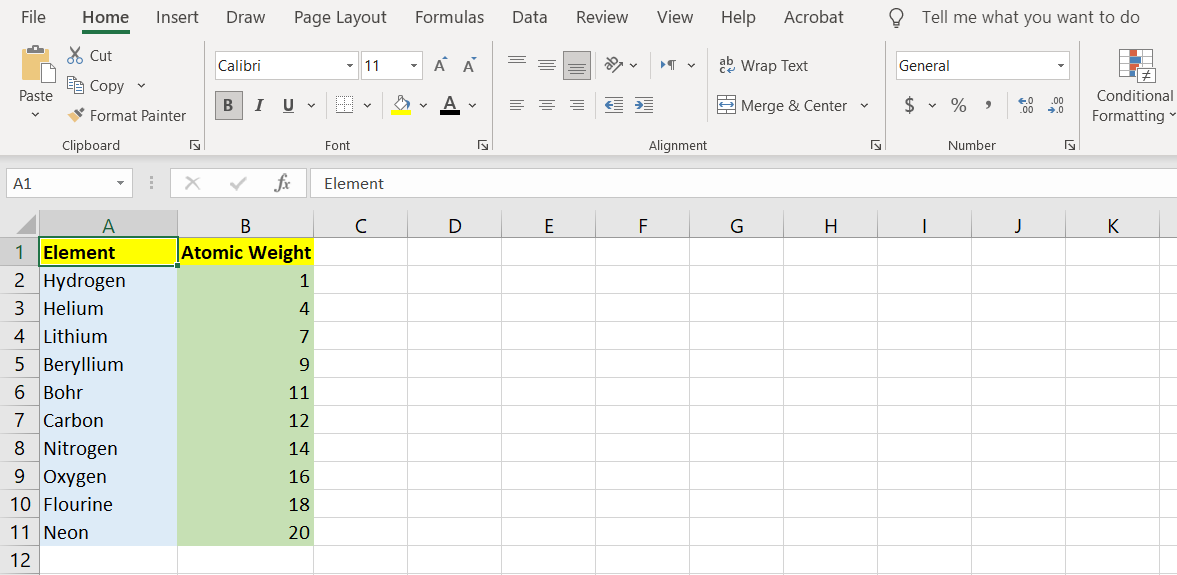
With wildcards, you can make a specific filter for your data in Excel. In this example spreadsheet, we have a list of the first ten elements from the periodic table. We’re going to make two different filters: First to get a list of elements that end with ium, and second to get a list of elements that only have four letters in their names.
- Click the header cell (A1) and then drag the selection over to the last element (A11).
- On your keyboard, press Ctrl + Shift + L. This will make a filter for that column.
- Click the arrow next to the header cell to open the filter menu.
- In the search box, enter *ium.
- Press Enter.
- Excel will now bring up all the elements in the list that end with ium.
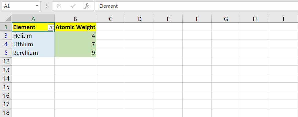
Now let’s run a filter to see which elements in this list have only four letters in their names. Since you’ve already created a filter, you’ll just need to adjust the content of the search box.
- Click the arrow next to the header cell. This will open the filter menu.
- In the search box, enter ????.
- Press Enter.
- Excel will now show only the elements that have four letters in their names.
To remove the filter and make all the cells visible:
- Click the arrow next to header cell.
- In the filter menu, under the search box, mark Select All.
- Press Enter.
If you’re curious about the filter tool and want to learn more about it, you should read our article on how to filter in Excel to display the data you want.
How to Search Data With Wildcards in Excel
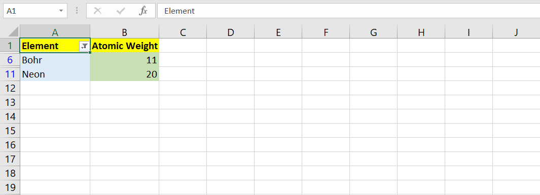
The Find and Replace tool in Excel supports wildcards and lets you use them to narrow down or expand your search. In the same spreadsheet, let’s try to search for elements that begin and end with N.
- Press Ctrl + F on your keyboard to bring up the Find and Replace window.
- In the text box in front of Find what enter N*N.
- Click Find All.
- The window will extend to display a list of cells that contain elements beginning and ending with N.
Now let’s run a more specific search. Which element in the list begins and ends with N, but has only four letters?
- Press Ctrl + F on your keyboard.
- In the text box, type N??N.
- Click Find All.
- The Find and Replace window will extend to show you the result.
How to Use Wildcards in Excel Formulas
While not all functions in Excel support wildcards, here are the six ones that do:
- AVERAGEIF
- COUNTIF
- SUMIF
- VLOOKUP
- SEARCH
- MATCH
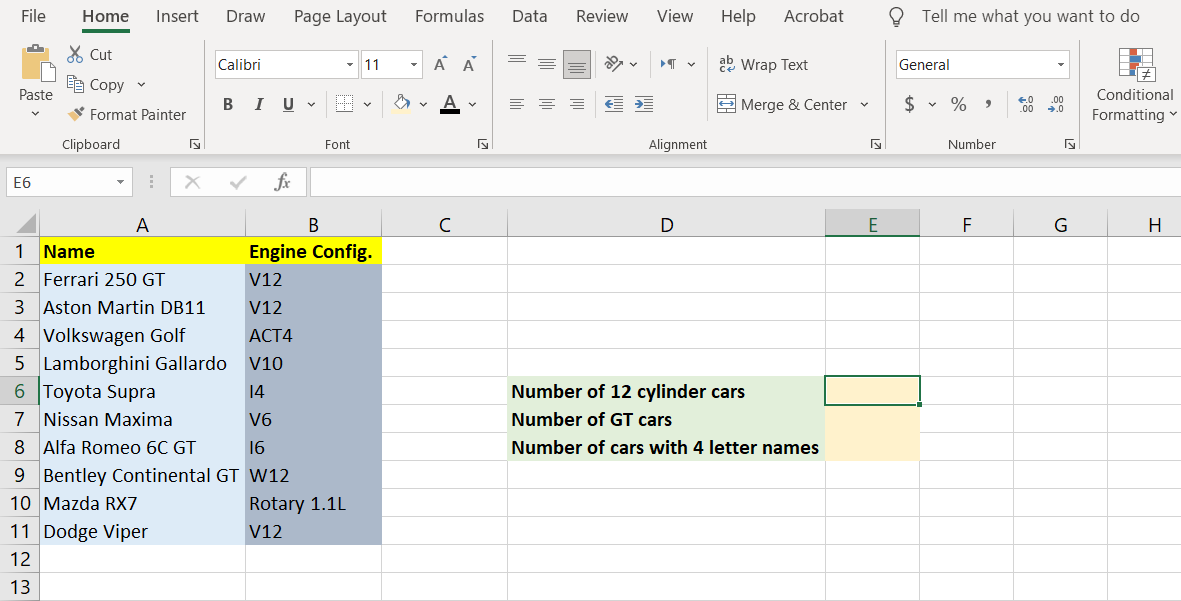
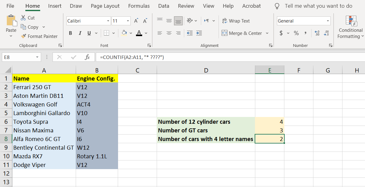
In this example, we have a list of cars and their engine configurations. We’re going to use the COUNTIF function to count three kinds of cars and then display the results in three separate cells. First, we can count how many cars are powered by 12-cylinder engines, then we can count how many cars have four-letter names.
Now that you have a grip on wildcards, it’s easy to guess that the first and second objectives can be accomplished solely with the asterisk.
- Select cell E6 (in our example).
- In the formula bar, enter the formula below:
=COUNTIF(B2:B11, "*12")
This formula will take the cells B2 to B11 and test them for the condition that the engine has 12 cylinders or not. Since this is regardless of the engine’s configuration, we need to include all the engines that end with 12, thus the asterisk.
- Press Enter.
- Excel will return the number of 12-cylinder cars in the list.
Counting the number of GT cars is done similarly. The only difference is an additional asterisk at the end of the name, which alerts us to any cars that do not end with GT but still contain the letter.
- Select cell E7.
- In the formula bar, enter the formula below:
=COUNTIF(A2:A11, "*GT*")
The formula will test cells A2 to A11 for the *GT* condition. This condition states that any cell that has the phrase GT in it, will be counted.
- Press Enter.
- Excel will return the number of GT cars.
The final objective is slightly different. To count the cars that have four-letter model names, we’re going to need the question mark wildcard.
- Select cell E8.
- In the formula bar, enter the formula below:
=COUNTIF(A2:A11, "* ????")
This formula will test the car names, the asterisk states that the car brand can be anything, whereas the four question marks make sure that the car model is in four letters.
- Press Enter.
- Excel will return the number of cars that have four-letter models. In this case, it’s going to be the Golf and the DB11.
Get the Data You Want With Wildcards
Wildcards are simple in nature, yet they have the potential to help you achieve sophisticated things in Excel. Coupled with formulas, they can make finding and counting cells much easier. If you’re interested in searching your spreadsheet more efficiently, there are a couple of Excel functions that you should start learning and using.
- Введение в подстановочный знак в Excel
Excel Wildcard (Оглавление)
- Введение в подстановочный знак в Excel
- Как использовать дикие символы в Excel?
Введение в подстановочный знак в Excel
Подстановочные знаки в Excel являются наиболее недооцененной функцией Excel, и большинство людей не знают об этом. Очень полезно знать эту функцию, поскольку она может сэкономить много времени и усилий, необходимых для проведения некоторых исследований в Excel. Мы узнаем о подстановочных знаках Excel подробно в этой статье.
В Excel есть 3 подстановочных знака:
- Звездочка (*)
- Вопросительный знак (?)
- Тильда (~)
Эти три символа подстановки определенно имеют разные цели друг от друга.
1. Звездочка (*) — Звездочка представляет любое количество символов в текстовой строке.
Например, когда вы набираете Br *, это может означать Break, Broke, Broken. Так что * после того, как Br может означать выбор только тех слов, которые начинаются с Break, не имеет значения, какие слова или количество символов будут после Br. Аналогичным образом вы можете начать поиск с Asterisk.
Например, * ing, это может означать начало, конец, начало. Так что * перед ing может означать выбор только тех слов, которые заканчиваются на ‘ing’, и не имеет значения, какие слова или количество символов присутствуют перед ing.
2. Знак вопроса (?) — Знак вопроса используется для одного символа.
Например, ? Ove может означать Dove или Move. Так что здесь знак вопроса представляет один символ, который является М или D.
3. Тильда (~) — мы уже видели два диких символа: звездочку (*) и вопросительный знак (?). Третий символ подстановки, который является тильдой (~), используется для определения символа подстановки. Мы не сталкивались со многими ситуациями, когда нам нужно использовать тильду (~), но полезно знать функцию в Excel.
Как использовать подстановочные знаки в Excel?
Давайте теперь посмотрим на приведенные ниже примеры использования подстановочных знаков в Excel.
Вы можете скачать этот шаблон шаблона подстановки здесь — Шаблон шаблона подстановки Excel
Пример # 1 — Фильтрация данных с подстановочными знаками
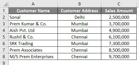
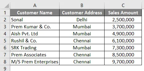
Предположим, вы работаете с данными о продажах, где у вас есть имя клиента, адрес клиента и сумма продаж, как показано на скриншоте ниже. В списке клиентов у вас есть разные компании материнской компании «Prem Enterprise». Поэтому, если мне нужно отфильтровать все компании Prem по имени клиента, я просто отфильтрую одну звездочку за Prem и одну звездочку за prem, которая будет выглядеть как «* Prem *», и опция поиска выдаст мне список всех компаний. который имеет Прем в названии компании.
Выполните следующие шаги, чтобы найти и отфильтровать компании, в названии которых есть «Прем».
- Перейдите на вкладку « Данные » в Excel.
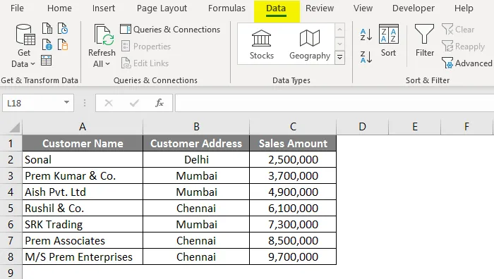
- Нажмите на опцию фильтра .
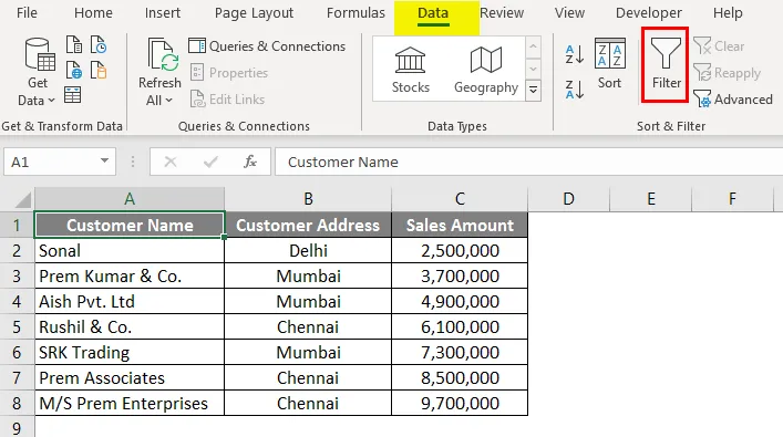
- После применения фильтра перейдите к столбцу «Имя клиента» и щелкните раскрывающийся список.
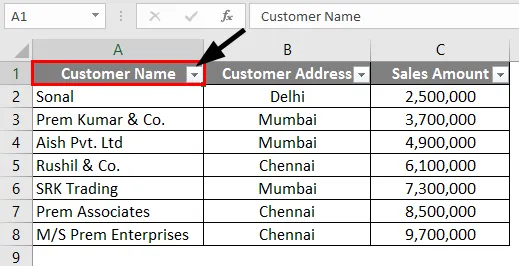
- В поле поиска введите « * Prem * » и нажмите «ОК».
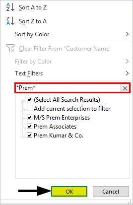
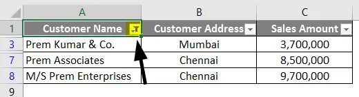
- Как видите, все три компании, в названии которых присутствует «Прем», были отфильтрованы и выбраны.
Пример № 2 — Найти и заменить, используя подстановочный знак
Область, где мы можем эффективно использовать символы подстановки, чтобы найти и заменить слова в Excel. Давайте возьмем аналогичный пример того, что мы использовали в Примере 1.
В первом примере мы отфильтровали названия компаний, в названии которых есть «Прем». Таким образом, в этом примере мы попытаемся найти название компаний, в названии которых есть «прем», и заменим название компании названием «Группа компаний Прем». Для этого вам необходимо выполнить следующие шаги.
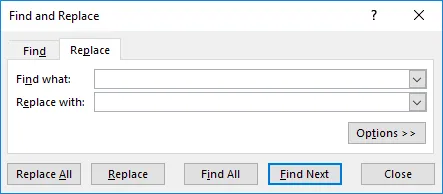
- Нажмите CTRL + H в Excel, и вы увидите открытый экран ниже.
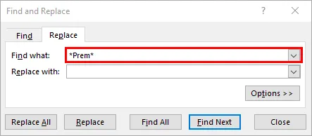
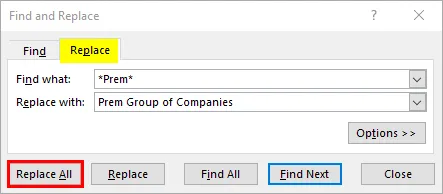
- В поле «Найти» введите слово « * Prem * ». Так что он должен искать название компаний, в названии которых есть «Прем».
- В поле «Заменить на» введите слово « Группа компаний Прем ».
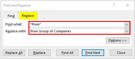
- Теперь нажмите кнопку « Заменить все », чтобы заменить все названия компаний, в названии которых есть «прем», на «Группа компаний Прем».
- После нажатия на кнопку «Заменить все», мы получим диалоговое окно ниже.
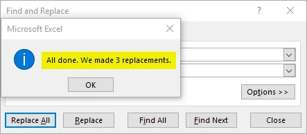
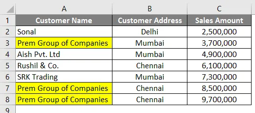
Вы видите, что названия компаний в строках 3, 7 и 8 изменены на «Группа компаний Прем».
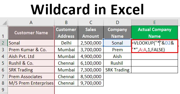
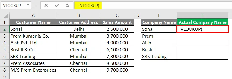
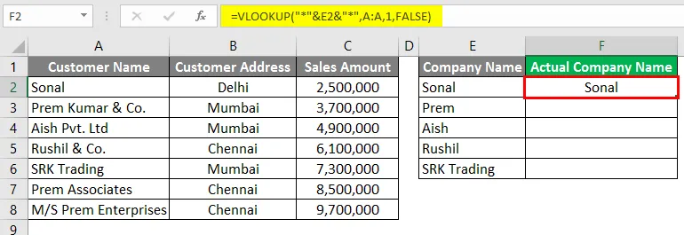
Пример № 3 — Vlookup с использованием подстановочного знака
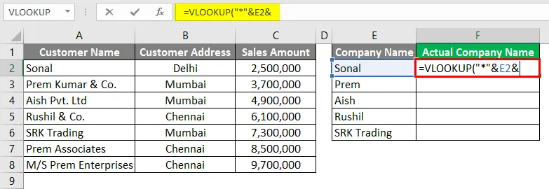
Так же, как мы привыкли находить и заменять с помощью подстановочных знаков, мы также можем использовать подстановочные знаки в Excel Vlookup. Мы возьмем аналогичный пример из примера 1. Но помимо данных в примере 1 у нас есть таблица с начальной ссылкой на название компании в столбце E.
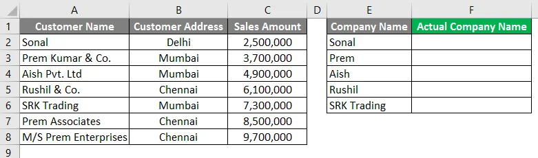
Обычный поиск здесь не будет работать, так как имена не совпадают в столбцах A и F. Таким образом, нам нужно выполнить поиск таким образом, чтобы он мог подобрать результат для названий компаний в столбце A.
Выполните следующие шаги, чтобы увидеть, как мы можем это сделать.
- Введите формулу для Vlookup в столбце F2, как показано на снимке экрана ниже.
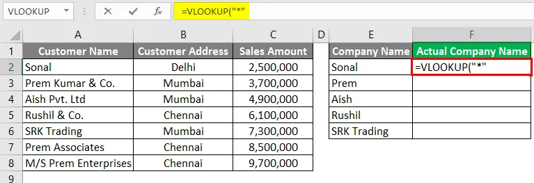
- Запустите значение Vlookup звездочкой между точками с запятой «*», как показано на снимке экрана ниже.
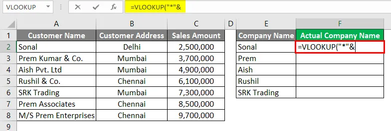
- Теперь введите «&», чтобы связать ссылку с ячейкой E2.
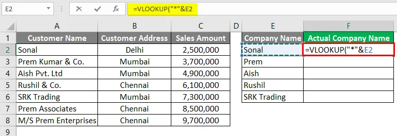
- Дайте ссылку на ячейку E2.
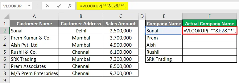
- Снова введите «&» после ссылки на ячейку.
- Теперь завершите значение Vlookup звездочкой между точками с запятой «*», как показано на скриншоте ниже.
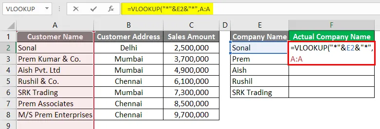
- Теперь для Table_Array в vlookup дайте ссылку на столбец A, чтобы он взял значение из столбца A.
- В столбце Индекс вы можете выбрать 1, так как нам нужно значение из самого столбца А.

- Для последнего условия в формуле VLOOKUP вы можете выбрать ЛОЖЬ для Точного соответствия.
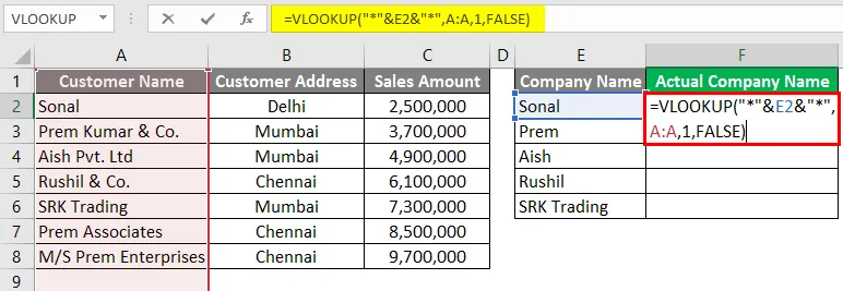
- Нажмите клавишу ввода.
- Теперь вы можете перетащить формулу в строку ниже и увидеть результат.
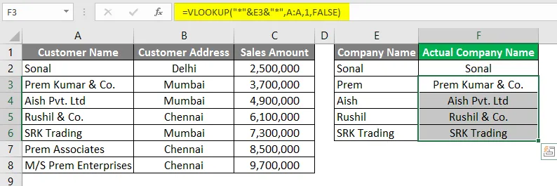
Как вы можете видеть, поиск выбрал значение из столбца A, хотя имена в столбце F не совпадали.
Что нужно помнить о подстановочных знаках в Excel
- Подстановочные знаки необходимо использовать осторожно, потому что это может дать результат другой опции, которая может поступать с той же логикой. Возможно, вам придется проверить эти параметры. Например, в примере 3, где мы ищем с помощью символа подстановки, было 3 компании с «Prem» в названии, но в результате поиска было зафиксировано только первое название компании, которое имеет «Prem» в названии в столбце A.
- Подстановочные знаки могут использоваться в других функциях Excel, таких как Vlookup, count, match и т. Д. Таким образом, вы можете использовать подстановочный знак многими инновационными способами.
- Мы также можем использовать комбинацию звездочки (*) и вопросительного знака (?) В некоторых ситуациях, если это необходимо.
Рекомендуемые статьи
Это руководство по подстановочным знакам в Excel. Здесь мы обсуждаем, как использовать символы подстановки в Excel вместе с практическими примерами и загружаемым шаблоном Excel. Вы также можете просмотреть наши другие предлагаемые статьи —
- Вставить календарь в Excel
- Максимальная формула в Excel
- Поле имени в Excel
- Переключение столбцов в Excel
- Как считать символы в Excel?
Содержание
- Подстановочный знак в Excel — Как использовать подстановочные знаки в Excel? (С типами)
- Введение в подстановочный знак в Excel
- Как использовать подстановочные знаки в Excel?
- Пример # 1 — Фильтрация данных с подстановочными знаками
- Пример № 2 — Найти и заменить, используя подстановочный знак
- Пример № 3 — Vlookup с использованием подстановочного знака
- Что нужно помнить о подстановочных знаках в Excel
- Рекомендуемые статьи
- Wildcard
- Available wildcards
- Example wildcard usage
- Functions that support wildcards
- Excel Wildcard Characters – What are these and How to Best Use it
- Excel Wildcard Characters – An Introduction
- Excel Wildcard Characters – Examples
- #1 Filter Data using Excel Wildcard Characters
- #2 Partial Lookup Using Wildcard Characters & VLOOKUP
- 3. Find and Replace Partial Matches
- 4. Count Non-blank Cells that Contain Text
Подстановочный знак в Excel — Как использовать подстановочные знаки в Excel? (С типами)

Excel Wildcard (Оглавление)
- Введение в подстановочный знак в Excel
- Как использовать дикие символы в Excel?
Введение в подстановочный знак в Excel
Подстановочные знаки в Excel являются наиболее недооцененной функцией Excel, и большинство людей не знают об этом. Очень полезно знать эту функцию, поскольку она может сэкономить много времени и усилий, необходимых для проведения некоторых исследований в Excel. Мы узнаем о подстановочных знаках Excel подробно в этой статье.
В Excel есть 3 подстановочных знака:
- Звездочка (*)
- Вопросительный знак (?)
- Тильда (
Эти три символа подстановки определенно имеют разные цели друг от друга.
1. Звездочка (*) — Звездочка представляет любое количество символов в текстовой строке.
Например, когда вы набираете Br *, это может означать Break, Broke, Broken. Так что * после того, как Br может означать выбор только тех слов, которые начинаются с Break, не имеет значения, какие слова или количество символов будут после Br. Аналогичным образом вы можете начать поиск с Asterisk.
Например, * ing, это может означать начало, конец, начало. Так что * перед ing может означать выбор только тех слов, которые заканчиваются на ‘ing’, и не имеет значения, какие слова или количество символов присутствуют перед ing.
2. Знак вопроса (?) — Знак вопроса используется для одного символа.
Например, ? Ove может означать Dove или Move. Так что здесь знак вопроса представляет один символ, который является М или D.
3. Тильда (
) — мы уже видели два диких символа: звездочку (*) и вопросительный знак (?). Третий символ подстановки, который является тильдой (
), используется для определения символа подстановки. Мы не сталкивались со многими ситуациями, когда нам нужно использовать тильду (
), но полезно знать функцию в Excel.
Как использовать подстановочные знаки в Excel?
Давайте теперь посмотрим на приведенные ниже примеры использования подстановочных знаков в Excel.
Вы можете скачать этот шаблон шаблона подстановки здесь — Шаблон шаблона подстановки Excel
Пример # 1 — Фильтрация данных с подстановочными знаками
Предположим, вы работаете с данными о продажах, где у вас есть имя клиента, адрес клиента и сумма продаж, как показано на скриншоте ниже. В списке клиентов у вас есть разные компании материнской компании «Prem Enterprise». Поэтому, если мне нужно отфильтровать все компании Prem по имени клиента, я просто отфильтрую одну звездочку за Prem и одну звездочку за prem, которая будет выглядеть как «* Prem *», и опция поиска выдаст мне список всех компаний. который имеет Прем в названии компании.

Выполните следующие шаги, чтобы найти и отфильтровать компании, в названии которых есть «Прем».
- Перейдите на вкладку « Данные » в Excel.

- Нажмите на опцию фильтра .

- После применения фильтра перейдите к столбцу «Имя клиента» и щелкните раскрывающийся список.

- В поле поиска введите « * Prem * » и нажмите «ОК».

- Как видите, все три компании, в названии которых присутствует «Прем», были отфильтрованы и выбраны.

Пример № 2 — Найти и заменить, используя подстановочный знак
Область, где мы можем эффективно использовать символы подстановки, чтобы найти и заменить слова в Excel. Давайте возьмем аналогичный пример того, что мы использовали в Примере 1.

В первом примере мы отфильтровали названия компаний, в названии которых есть «Прем». Таким образом, в этом примере мы попытаемся найти название компаний, в названии которых есть «прем», и заменим название компании названием «Группа компаний Прем». Для этого вам необходимо выполнить следующие шаги.
- Нажмите CTRL + H в Excel, и вы увидите открытый экран ниже.

- В поле «Найти» введите слово « * Prem * ». Так что он должен искать название компаний, в названии которых есть «Прем».

- В поле «Заменить на» введите слово « Группа компаний Прем ».

- Теперь нажмите кнопку « Заменить все », чтобы заменить все названия компаний, в названии которых есть «прем», на «Группа компаний Прем».

- После нажатия на кнопку «Заменить все», мы получим диалоговое окно ниже.

Вы видите, что названия компаний в строках 3, 7 и 8 изменены на «Группа компаний Прем».

Пример № 3 — Vlookup с использованием подстановочного знака
Так же, как мы привыкли находить и заменять с помощью подстановочных знаков, мы также можем использовать подстановочные знаки в Excel Vlookup. Мы возьмем аналогичный пример из примера 1. Но помимо данных в примере 1 у нас есть таблица с начальной ссылкой на название компании в столбце E.

Обычный поиск здесь не будет работать, так как имена не совпадают в столбцах A и F. Таким образом, нам нужно выполнить поиск таким образом, чтобы он мог подобрать результат для названий компаний в столбце A.
Выполните следующие шаги, чтобы увидеть, как мы можем это сделать.
- Введите формулу для Vlookup в столбце F2, как показано на снимке экрана ниже.

- Запустите значение Vlookup звездочкой между точками с запятой «*», как показано на снимке экрана ниже.

- Теперь введите «&», чтобы связать ссылку с ячейкой E2.

- Дайте ссылку на ячейку E2.

- Снова введите «&» после ссылки на ячейку.

- Теперь завершите значение Vlookup звездочкой между точками с запятой «*», как показано на скриншоте ниже.

- Теперь для Table_Array в vlookup дайте ссылку на столбец A, чтобы он взял значение из столбца A.

- В столбце Индекс вы можете выбрать 1, так как нам нужно значение из самого столбца А.

- Для последнего условия в формуле VLOOKUP вы можете выбрать ЛОЖЬ для Точного соответствия.


- Теперь вы можете перетащить формулу в строку ниже и увидеть результат.

Как вы можете видеть, поиск выбрал значение из столбца A, хотя имена в столбце F не совпадали.
Что нужно помнить о подстановочных знаках в Excel
- Подстановочные знаки необходимо использовать осторожно, потому что это может дать результат другой опции, которая может поступать с той же логикой. Возможно, вам придется проверить эти параметры. Например, в примере 3, где мы ищем с помощью символа подстановки, было 3 компании с «Prem» в названии, но в результате поиска было зафиксировано только первое название компании, которое имеет «Prem» в названии в столбце A.
- Подстановочные знаки могут использоваться в других функциях Excel, таких как Vlookup, count, match и т. Д. Таким образом, вы можете использовать подстановочный знак многими инновационными способами.
- Мы также можем использовать комбинацию звездочки (*) и вопросительного знака (?) В некоторых ситуациях, если это необходимо.
Рекомендуемые статьи
Это руководство по подстановочным знакам в Excel. Здесь мы обсуждаем, как использовать символы подстановки в Excel вместе с практическими примерами и загружаемым шаблоном Excel. Вы также можете просмотреть наши другие предлагаемые статьи —
- Вставить календарь в Excel
- Максимальная формула в Excel
- Поле имени в Excel
- Переключение столбцов в Excel
- Как считать символы в Excel?
Источник
Wildcard
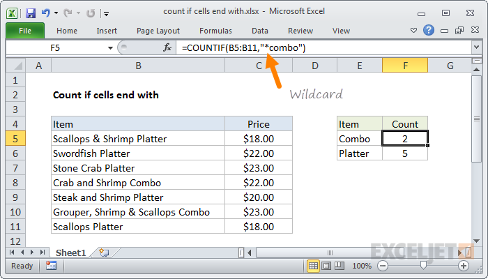
A wildcard is a special character that lets you perform «fuzzy» matching on text in your Excel formulas. For example, this formula:
counts all cells in the range B5:B11 that end with the text «combo». And this formula:
Counts all cells in A1:A100 that contain exactly 3 characters.
Available wildcards
Excel has 3 wildcards you can use in your formulas:
- Asterisk (*) — zero or more characters
- Question mark (?) — any one character
- Tilde (
) — escape for literal character (
*) a literal question mark (
?), or a literal tilde (
Example wildcard usage
| Usage | Behavior | Will match |
|---|---|---|
| ? | Any one character | «A», «B», «c», «z», etc. |
| ?? | Any two characters | «AA», «AZ», «zz», etc. |
| . | Any three characters | «Jet», «AAA», «ccc», etc. |
| * | Any characters | «apple», «APPLE», «A100», etc. |
| *th | Ends in «th» | «bath», «fourth», etc. |
| c* | Starts with «c» | «Cat», «CAB», «cindy», «candy», etc. |
| ?* | At least one character | «a», «b», «ab», «ABCD», etc. |
| . -?? | 5 characters with hypen | «ABC-99″,»100-ZT», etc. |
| * |
? Ends in question mark «Hello?», «Anybody home?», etc. *xyz* Contains «xyz» «code is XYZ», «100-XYZ», «XyZ90», etc.
Wildcards only work with text. For numeric data, you can use logical operators.
Functions that support wildcards
Not all functions allow wildcards. Here is a list of the most common functions that do:
Источник
Excel Wildcard Characters – What are these and How to Best Use it
Watch Video on Excel Wildcard Characters
There are only 3 Excel wildcard characters (asterisk, question mark, and tilde) and a lot can be done using these.
In this tutorial, I will show you four examples where these Excel wildcard characters are absolute lifesavers.
This Tutorial Covers:
Excel Wildcard Characters – An Introduction
Wildcards are special characters that can take any place of any character (hence the name – wildcard).
There are three wildcard characters in Excel:
- * (asterisk) – It represents any number of characters . For example, Ex* could mean Excel, Excels, Example, Expert, etc.
- ? (question mark) – It represents one single character. For example, Tr?mp could mean Trump or Tramp.
(tilde) – It is used to identify a wildcard character (
, *, ?) in the text. For example, let’s say you want to find the exact phrase Excel* in a list. If you use Excel* as the search string, it would give you any word that has Excel at the beginning followed by any number of characters (such as Excel, Excels, Excellent). To specifically look for excel*, we need to use
. So our search string would be excel
*. Here, the presence of
ensures that excel reads the following character as is, and not as a wildcard.
Note: I have not come across many situations where you need to use
. Nevertheless, it is a good to know feature.
Now let’s go through four awesome examples where wildcard characters do all the heavy lifting.
Excel Wildcard Characters – Examples
Now let’s look at four practical examples where Excel wildcard characters can be mighty useful:
- Filtering data using a wildcard character.
- Partial Lookup using wildcard character and VLOOKUP.
- Find and Replace Partial Matches.
- Count Non-blank cells that contain text.
#1 Filter Data using Excel Wildcard Characters
Excel wildcard characters come in handy when you have huge data sets and you want to filter data based on a condition.
Suppose you have a dataset as shown below:

You can use the asterisk (*) wildcard character in data filter to get a list of companies that start with the alphabet A.
Here is how to do this:
This will instantly filter the results and give you 3 names – ABC Ltd., Amazon.com, and Apple Stores.

How does it work? – When you add an asterisk (*) after A, Excel would filter anything that starts with A. This is because an asterisk (being an Excel wildcard character) can represent any number of characters.
Now with the same methodology, you can use various criteria to filter results.
For example, if you want to filter companies that begin with the alphabet A and contain the alphabet C in it, use the string A*C. This will give you only 2 results – ABC Ltd. and Amazon.com.
If you use A?C instead, you will only get ABC Ltd as the result (as only one character is allowed between ‘a’ and ‘c’)
#2 Partial Lookup Using Wildcard Characters & VLOOKUP
Partial look-up is needed when you have to look for a value in a list and there isn’t an exact match.
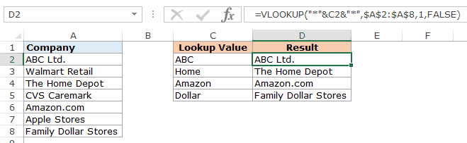
For example, suppose you have a data set as shown below, and you want to look for the company ABC in a list, but the list has ABC Ltd instead of ABC.
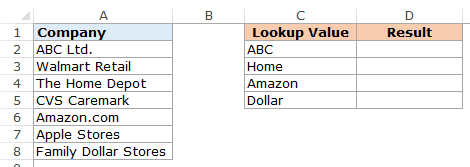
You can not use the regular VLOOKUP function in this case as the lookup value does not have an exact match.
If you use VLOOKUP with an approximate match, it will give you the wrong results.
However, you can use a wildcard character within VLOOKUP function to get the right results:
Enter the following formula in cell D2 and drag it for other cells:
How does this formula work?
In the above formula, instead of using the lookup value as is, it is flanked on both sides with the Excel wildcard character asterisk (*) – “*”&C2&”*”
This tells excel that it needs to look for any text that contains the word in C2. It could have any number of characters before or after the text in C2.
Hence, the formula looks for a match, and as soon as it gets a match, it returns that value.
3. Find and Replace Partial Matches
Excel Wildcard characters are quite versatile.
You can use it in a complex formula as well as in basic functionality such as Find and Replace.
Suppose you have the data as shown below:

In the above data, the region has been entered in different ways (such as North-West, North West, NorthWest).
This is often the case with sales data.
To clean this data and make it consistent, we can use Find and Replace with Excel wildcard characters.
Here is how to do this:
- Select the data where you want to find and replace text.
- Go to Home –> Find & Select –> Go To. This will open the Find and Replace dialogue box. (You can also use the keyboard shortcut – Control + H).
- Enter the following text in the find and replace dialogue box:
- Find what: North*W*
- Replace with: North-West

- Click on Replace All.

This will instantly change all the different formats and make it consistent to North-West.

How does this Work?
In the Find field, we have used North*W* which will find any text that has the word North and contains the alphabet ‘W’ anywhere after it.
Hence, it covers all the scenarios (NorthWest, North West, and North-West).
Find and Replace finds all these instances and changes it to North-West and makes it consistent.
4. Count Non-blank Cells that Contain Text
I know you are smart and you thinking that Excel already has an inbuilt function to do this.
You’re absolutely right!!
This can be done using the COUNTA function.
BUT… There is one small problem with it.
A lot of times when you import data or use other people’s worksheet, you will notice that there are empty cells while that might not be the case.
These cells look blank but have =”” in it. The trouble is that the
The trouble is that the COUNTA function does not consider this as an empty cell (it counts it as text).
See the example below:

In the above example, I use the COUNTA function to find cells that are not empty and it returns 11 and not 10 (but you can clearly see only 10 cells have text).
The reason, as I mentioned, is that it doesn’t consider A11 as empty (while it should).
But that is how Excel works.
The fix is to use the Excel wildcard character within the formula.
Below is a formula using the COUNTIF function that only counts cells that have text in it:
This formula tells excel to count only if the cell has at least one character.
In the ?* combo:
- ? (question mark) ensures that at least one character is present.
- * (asterisk) makes room for any number of additional characters.
Note: The above formula works when only have text values in the cells. If you have a list that has both text as well as numbers, use the following formula:
Similarly, you can use wildcards in a lot of other Excel functions, such as IF(), SUMIF(), AVERAGEIF(), and MATCH().
It’s also interesting to note that while you can use the wildcard characters in the SEARCH function, you can’t use it in FIND function.
Hope these examples give you a flair of the versatility and power of Excel wildcard characters.
If you have any other innovative way to use it, do share it with me in the comments section.
You May Find the Following Excel Tutorials Useful:
Источник
A wildcard is a special character that lets you perform «fuzzy» matching on text in your Excel formulas. For example, this formula:
=COUNTIF(B5:B11,"*combo")
counts all cells in the range B5:B11 that end with the text «combo». And this formula:
=COUNTIF(A1:A100,"???")
Counts all cells in A1:A100 that contain exactly 3 characters.
Available wildcards
Excel has 3 wildcards you can use in your formulas:
- Asterisk (*) — zero or more characters
- Question mark (?) — any one character
- Tilde (~) — escape for literal character (~*) a literal question mark (~?), or a literal tilde (~~).
Note: wildcards only work with text, not numbers.
Example wildcard usage
| Usage | Behavior | Will match |
|---|---|---|
| ? | Any one character | «A», «B», «c», «z», etc. |
| ?? | Any two characters | «AA», «AZ», «zz», etc. |
| ??? | Any three characters | «Jet», «AAA», «ccc», etc. |
| * | Any characters | «apple», «APPLE», «A100», etc. |
| *th | Ends in «th» | «bath», «fourth», etc. |
| c* | Starts with «c» | «Cat», «CAB», «cindy», «candy», etc. |
| ?* | At least one character | «a», «b», «ab», «ABCD», etc. |
| ???-?? | 5 characters with hypen | «ABC-99″,»100-ZT», etc. |
| *~? | Ends in question mark | «Hello?», «Anybody home?», etc. |
| *xyz* | Contains «xyz» | «code is XYZ», «100-XYZ», «XyZ90», etc. |
Wildcards only work with text. For numeric data, you can use logical operators.
More general information on formula criteria here.
Functions that support wildcards
Not all functions allow wildcards. Here is a list of the most common functions that do:
- AVERAGEIF, AVERAGEIFS
- COUNTIF, COUNTIFS
- MAXIFS, MINIFS
- SUMIF, SUMIFS
- VLOOKUP, HLOOKUP
- MATCH
- SEARCH