Width of a cell in excel - Word и Excel - помощь в работе с программами

If you find yourself needing to expand or reduce Excel’s row widths and column heights, there are several ways to adjust them. The table below shows the minimum, maximum and default sizes for each based on a point scale.

Type	Min	Max	Default
Column	0 (hidden)	255	8.43
Row	0 (hidden)	409	15.00

Notes:

If you are working in Page Layout view (View tab, Workbook Views group, Page Layout button), you can specify a column width or row height in inches, centimeters and millimeters. The measurement unit is in inches by default. Go to File > Options > Advanced > Display > select an option from the Ruler Units list. If you switch to Normal view, then column widths and row heights will be displayed in points.
Individual rows and columns can only have one setting. For example, a single column can have a 25 point width, but it can’t be 25 points wide for one row, and 10 points for another.

Set a column to a specific width

Select the column or columns that you want to change.
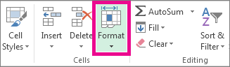
On the Home tab, in the Cells group, click Format.
Under Cell Size, click Column Width.
In the Column width box, type the value that you want.
Click OK.

Tip: To quickly set the width of a single column, right-click the selected column, click Column Width, type the value that you want, and then click OK.

Select the column or columns that you want to change.
On the Home tab, in the Cells group, click Format.
Under Cell Size, click AutoFit Column Width.

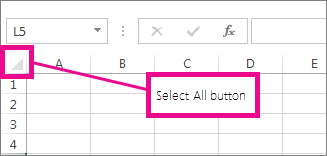
Note: To quickly autofit all columns on the worksheet, click the Select All button, and then double-click any boundary between two column headings.

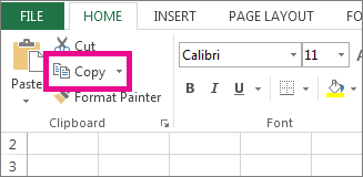
Select a cell in the column that has the width that you want to use.
Press Ctrl+C, or on the Home tab, in the Clipboard group, click Copy.
Right-click a cell in the target column, point to Paste Special, and then click the Keep Source Columns Widths button.

The value for the default column width indicates the average number of characters of the standard font that fit in a cell. You can specify a different number for the default column width for a worksheet or workbook.

Do one of the following:
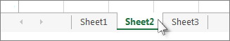
- To change the default column width for a worksheet, click its sheet tab.
- To change the default column width for the entire workbook, right-click a sheet tab, and then click Select All Sheets on the shortcut menu.
On the Home tab, in the Cells group, click Format.
Under Cell Size, click Default Width.
In the Standard column width box, type a new measurement, and then click OK.

Do one of the following:

To change the width of one column, drag the boundary on the right side of the column heading until the column is the width that you want.
To change the width of multiple columns, select the columns that you want to change, and then drag a boundary to the right of a selected column heading.
To change the width of columns to fit the contents, select the column or columns that you want to change, and then double-click the boundary to the right of a selected column heading.
To change the width of all columns on the worksheet, click the Select All button, and then drag the boundary of any column heading.

Select the row or rows that you want to change.
On the Home tab, in the Cells group, click Format.
Under Cell Size, click Row Height.
In the Row height box, type the value that you want, and then click OK.

Select the row or rows that you want to change.
On the Home tab, in the Cells group, click Format.
Under Cell Size, click AutoFit Row Height.

Tip: To quickly autofit all rows on the worksheet, click the Select All button, and then double-click the boundary below one of the row headings.

Do one of the following:

To change the row height of one row, drag the boundary below the row heading until the row is the height that you want.
To change the row height of multiple rows, select the rows that you want to change, and then drag the boundary below one of the selected row headings.
To change the row height for all rows on the worksheet, click the Select All button, and then drag the boundary below any row heading.
To change the row height to fit the contents, double-click the boundary below the row heading.

Top of Page

If you prefer to work with column widths and row heights in inches, you should work in Page Layout view (View tab, Workbook Views group, Page Layout button). In Page Layout view, you can specify a column width or row height in inches. In this view, inches are the measurement unit by default, but you can change the measurement unit to centimeters or millimeters.

In Excel 2007, click the Microsoft Office Button > Excel Options> Advanced.
In Excel 2010, go to File > Options > Advanced.

Set a column to a specific width

Select the column or columns that you want to change.
On the Home tab, in the Cells group, click Format.
Under Cell Size, click Column Width.
In the Column width box, type the value that you want.

Select the column or columns that you want to change.
On the Home tab, in the Cells group, click Format.
Under Cell Size, click AutoFit Column Width.

Tip To quickly autofit all columns on the worksheet, click the Select All button and then double-click any boundary between two column headings.

Select a cell in the column that has the width that you want to use.
On the Home tab, in the Clipboard group, click Copy, and then select the target column.
On the Home tab, in the Clipboard group, click the arrow below Paste, and then click Paste Special.
Under Paste, select Column widths.

Do one of the following:
- To change the default column width for a worksheet, click its sheet tab.
- To change the default column width for the entire workbook, right-click a sheet tab, and then click Select All Sheets on the shortcut menu.
On the Home tab, in the Cells group, click Format.
Under Cell Size, click Default Width.
In the Default column width box, type a new measurement.

Tip If you want to define the default column width for all new workbooks and worksheets, you can create a workbook template or a worksheet template, and then base new workbooks or worksheets on those templates. For more information, see Save a workbook or worksheet as a template.

Do one of the following:

To change the width of one column, drag the boundary on the right side of the column heading until the column is the width that you want.
To change the width of multiple columns, select the columns that you want to change, and then drag a boundary to the right of a selected column heading.
To change the width of columns to fit the contents, select the column or columns that you want to change, and then double-click the boundary to the right of a selected column heading.
To change the width of all columns on the worksheet, click the Select All button, and then drag the boundary of any column heading.

Select the row or rows that you want to change.
On the Home tab, in the Cells group, click Format.
Under Cell Size, click Row Height.
In the Row height box, type the value that you want.

Select the row or rows that you want to change.
On the Home tab, in the Cells group, click Format.
Under Cell Size, click AutoFit Row Height.

Tip To quickly autofit all rows on the worksheet, click the Select All button and then double-click the boundary below one of the row headings.

Do one of the following:

To change the row height of one row, drag the boundary below the row heading until the row is the height that you want.
To change the row height of multiple rows, select the rows that you want to change, and then drag the boundary below one of the selected row headings.
To change the row height for all rows on the worksheet, click the Select All button, and then drag the boundary below any row heading.
To change the row height to fit the contents, double-click the boundary below the row heading.

Top of Page

Варианты изменения величины элементов листа

Сразу нужно отметить, что по естественным причинам изменить величину только одной ячейки не получится. Изменяя высоту одного элемента листа, мы тем самым изменяем высоту всей строки, где он расположен. Изменяя его ширину – мы изменяем ширину того столбца, где он находится. По большому счету в Экселе не так уж и много вариантов изменения размера ячейки. Это можно сделать либо вручную перетащив границы, либо задав конкретный размер в числовом выражении с помощью специальной формы. Давайте узнаем о каждом из этих вариантов более подробно.

Способ 1: перетаскивание границ

Изменение величины ячейки путем перетаскивания границ является наиболее простым и интуитивно понятным вариантом.

Для того, чтобы увеличить или уменьшить высоту ячейки, наводим курсор на нижнюю границу сектора на вертикальной панели координат той строчки, в которой она находится. Курсор должен трансформироваться в стрелку, направленную в обе стороны. Делаем зажим левой кнопки мыши и тянем курсор вверх (если следует сузить) или вниз (если требуется расширить).

После того, как высота ячейки достигла приемлемого уровня, отпускаем кнопку мыши.

Изменение ширины элементов листа путем перетягивания границ происходит по такому же принципу.

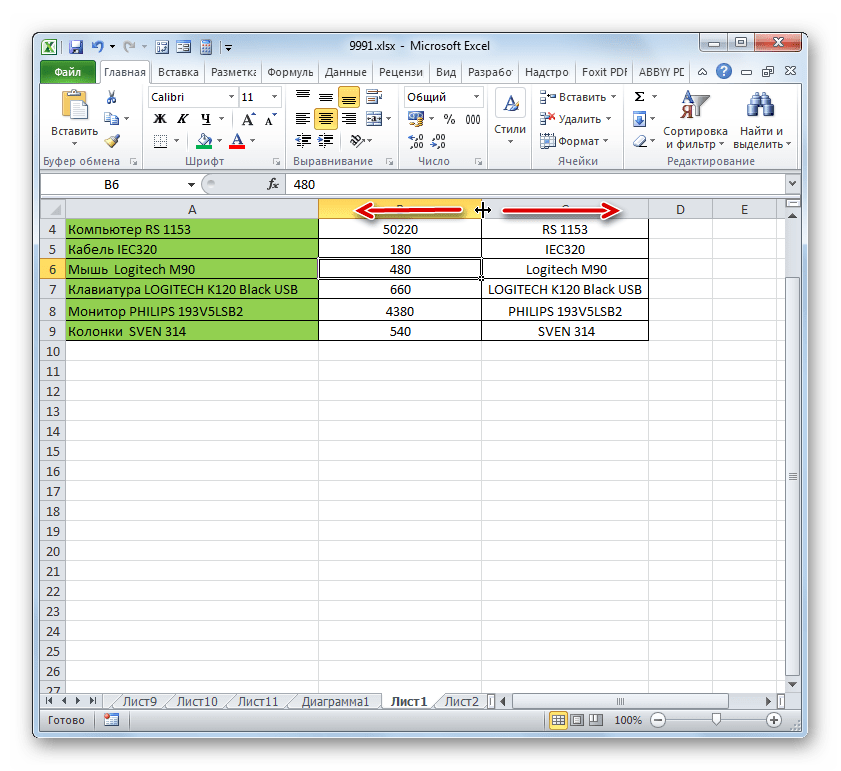
Наводим курсор на правую границу сектора столбца на горизонтальной панели координат, где она находится. После преобразования курсора в двунаправленную стрелку производим зажим левой кнопки мыши и тащим его вправо (если границы требуется раздвинуть) или влево (если границы следует сузить).

По достижении приемлемой величины объекта, у которого мы изменяем размер, отпускаем кнопку мышки.

Если вы хотите изменить размеры нескольких объектов одновременно, то в этом случае требуется сначала выделить соответствующие им сектора на вертикальной или горизонтальной панели координат, в зависимости от того, что требуется изменить в конкретном случае: ширину или высоту.

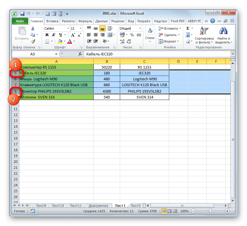
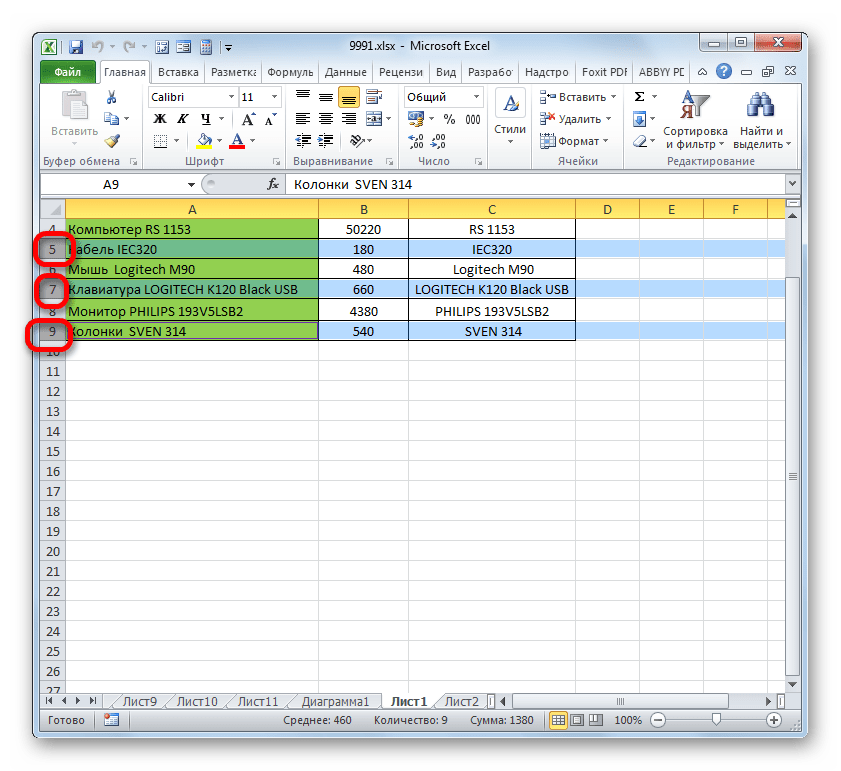
Процедура выделения, как для строк, так и для столбцов практически одинакова. Если нужно увеличить расположенные подряд ячейки, то кликаем левой кнопкой мыши по тому сектору на соответствующей панели координат, в котором находится первая из них. После этого точно так же кликаем по последнему сектору, но на этот раз уже одновременно зажав клавишу Shift. Таким образом, будут выделены все строки или столбцы, которые расположены между этими секторами.

Если нужно выделить ячейки, которые не являются смежными между собой, то в этом случае алгоритм действий несколько иной. Кликаем левой кнопкой мыши по одному из секторов столбца или строки, которые следует выделить. Затем, зажав клавишу Ctrl, клацаем по всем остальным элементам, находящимся на определенной панели координат, которые соответствуют объектам, предназначенным для выделения. Все столбцы или строки, где находятся эти ячейки, будут выделены.

Затем, нам следует для изменения размера нужных ячеек переместить границы. Выбираем соответствующую границу на панели координат и, дождавшись появления двунаправленной стрелки, зажимаем левую кнопку мыши. Затем передвигаем границу на панели координат в соответствии с тем, что именно нужно сделать (расширить (сузить) ширину или высоту элементов листа) точно так, как было описано в варианте с одиночным изменением размера.

После того, как размер достигнет нужной величины, отпускаем мышку. Как можно увидеть, изменилась величина не только строки или столбца, с границами которых была произведена манипуляция, но и всех ранее выделенных элементов.

Способ 2: изменение величины в числовом выражении

Теперь давайте выясним, как можно изменить размер элементов листа, задав его конкретным числовым выражением в специально предназначенном для этих целей поле.

В Экселе по умолчанию размер элементов листа задается в специальных единицах измерения. Одна такая единица равна одному символу. По умолчанию ширина ячейки равна 8,43. То есть, в видимую часть одного элемента листа, если его не расширять, можно вписать чуть больше 8 символов. Максимальная ширина составляет 255. Большее количество символов в ячейку вписать не получится. Минимальная ширина равна нулю. Элемент с таким размером является скрытым.

Высота строки по умолчанию равна 15 пунктам. Её размер может варьироваться от 0 до 409 пунктов.

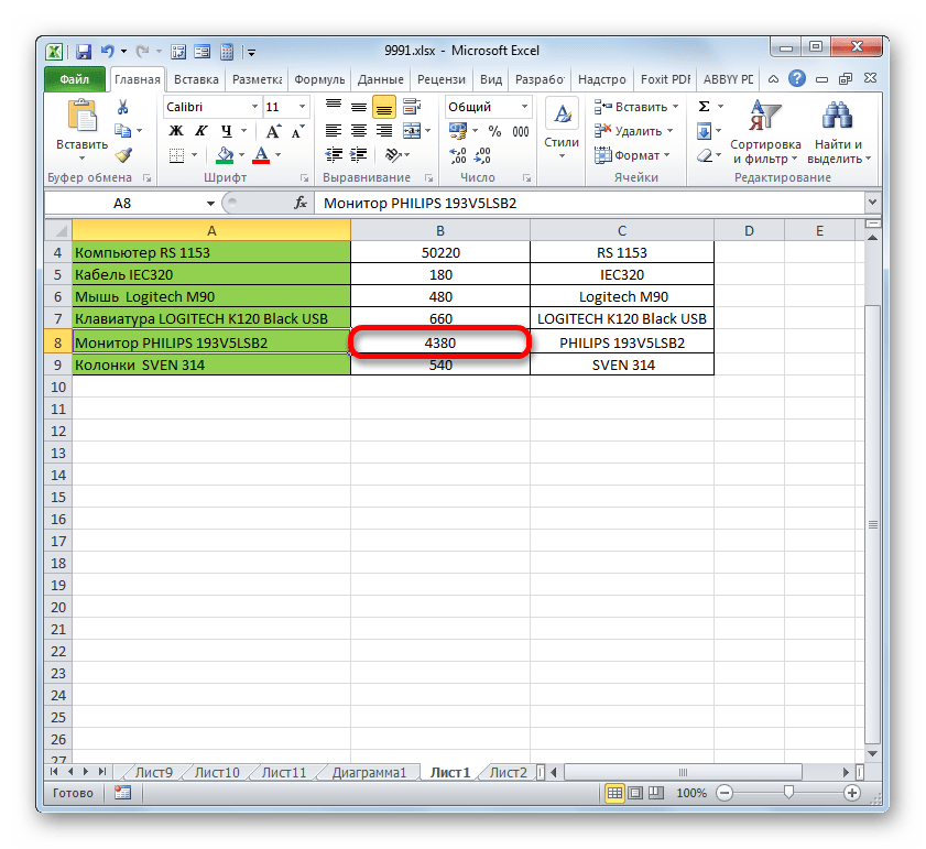
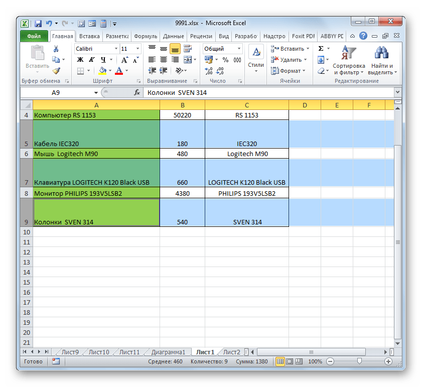
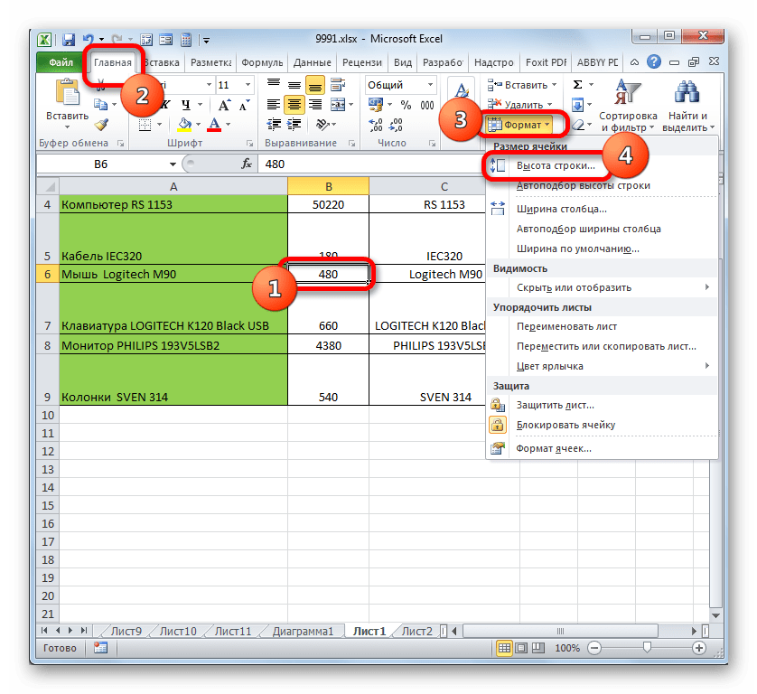
Для того, чтобы изменить высоту элемента листа, выделяем его. Затем, расположившись во вкладке «Главная», клацаем по значку «Формат», который размещен на ленте в группе «Ячейки». Из выпадающего списка выбираем вариант «Высота строки».

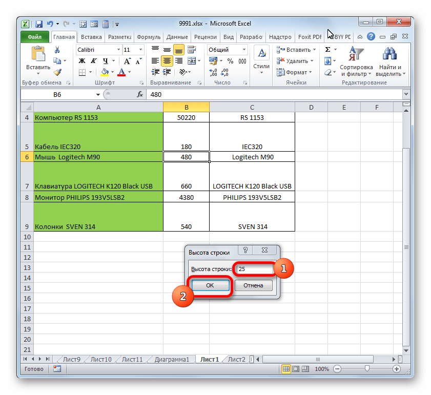
Открывается маленькое окошко с полем «Высота строки». Именно тут мы должны задать нужную величину в пунктах. Выполняем действие и клацаем по кнопке «OK».

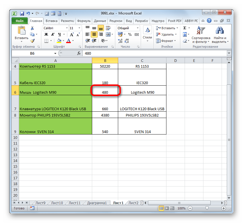
После этого высота строки, в которой находится выделенный элемент листа, будет изменена до указанной величины в пунктах.

Примерно таким же образом можно изменить и ширину столбца.

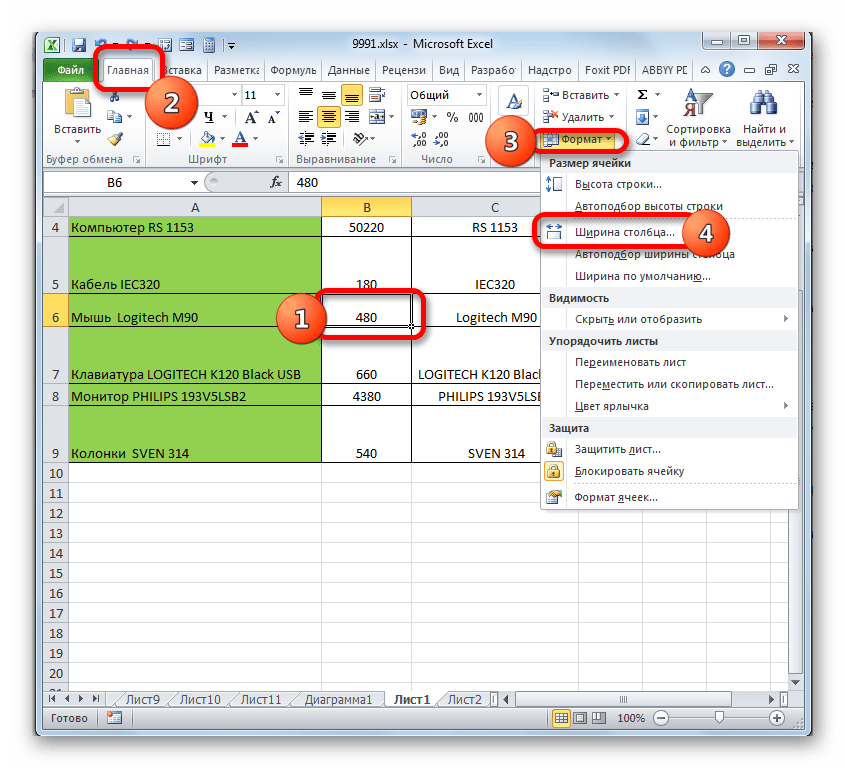
Выделяем элемент листа, в котором следует изменить ширину. Пребывая во вкладке «Главная» щелкаем по кнопке «Формат». В открывшемся меню выбираем вариант «Ширина столбца…».

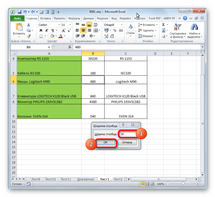
Открывается практически идентичное окошко тому, которое мы наблюдали в предыдущем случае. Тут так же в поле нужно задать величину в специальных единицах, но только на этот раз она будет указывать ширину столбца. После выполнения данных действий жмем на кнопку «OK».

После выполнения указанной операции ширина столбца, а значит и нужной нам ячейки, будет изменена.

Существуют и другой вариант изменить размер элементов листа, задав указанную величину в числовом выражении.

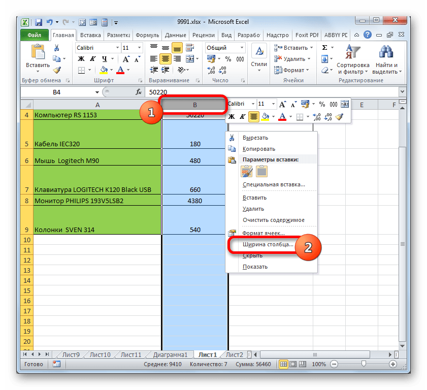
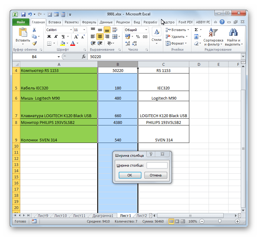
Для этого следует выделить столбец или строку, в которой находится нужная ячейка, в зависимости от того, что вы хотите изменить: ширину и высоту. Выделение производится через панель координат с помощью тех вариантов, которые мы рассматривали в Способе 1. Затем клацаем по выделению правой кнопкой мыши. Активируется контекстное меню, где нужно выбрать пункт «Высота строки…» или «Ширина столбца…».

Открывается окошко размера, о котором шла речь выше. В него нужно вписать желаемую высоту или ширину ячейки точно так же, как было описано ранее.

Впрочем, некоторых пользователей все-таки не устраивает принятая в Экселе система указания размера элементов листа в пунктах, выраженных в количестве символов. Для этих пользователей существует возможность переключения на другую величину измерения.

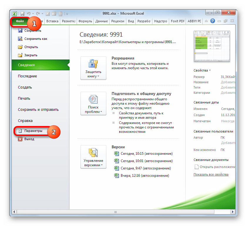
Переходим во вкладку «Файл» и выбираем пункт «Параметры» в левом вертикальном меню.

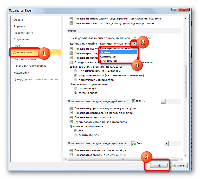
Запускается окно параметров. В его левой части расположено меню. Переходим в раздел «Дополнительно». В правой части окна расположены различные настройки. Прокручиваем полосу прокрутки вниз и ищем блок инструментов «Экран». В этом блоке расположено поле «Единицы на линейке». Кликаем по нему и из выпадающего списка выбираем более подходящую единицу измерения. Существуют следующие варианты:
- Сантиметры;
- Миллиметры;
- Дюймы;
- Единицы по умолчанию.
После того, как выбор сделан, для вступления изменений в силу жмем по кнопке «OK» в нижней части окна.

Теперь вы сможете регулировать изменение величины ячеек при помощи тех вариантов, которые указаны выше, оперируя выбранной единицей измерения.

Способ 3: автоматическое изменение размера

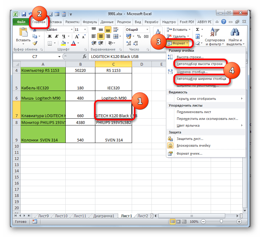
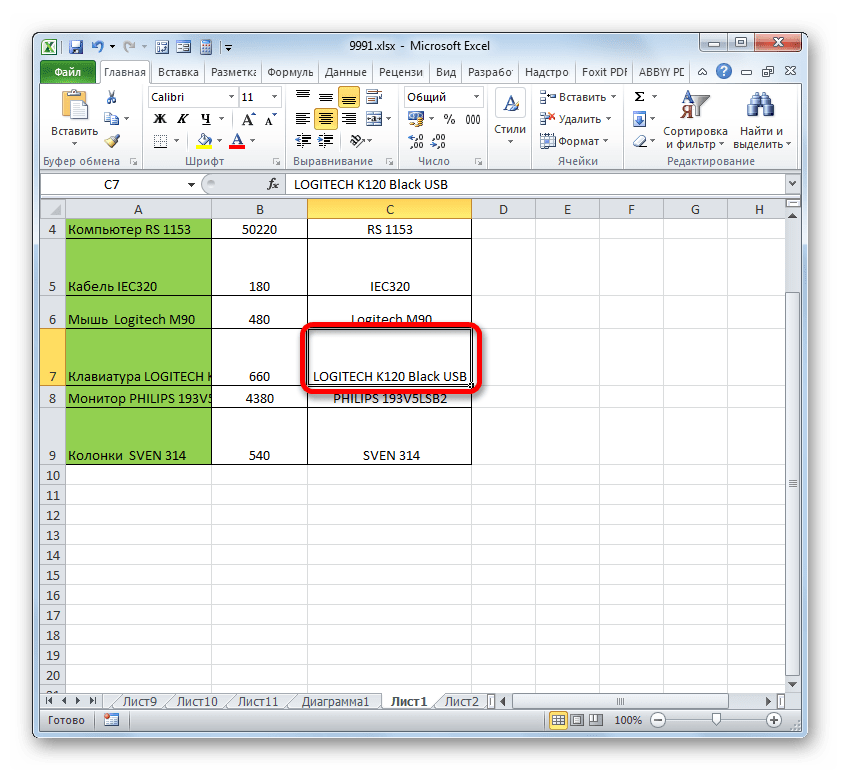
Но, согласитесь, что не совсем удобно всегда вручную менять размеры ячеек, подстраивая их под конкретное содержимое. К счастью, в Excel предусмотрена возможность автоматического изменения размеров элементов листа, согласно величине тех данных, которые они содержат.

Выделяем ячейку или группу, данные в которой не помещаются в элемент листа, содержащего их. Во вкладке «Главная» клацаем по знакомой кнопке «Формат». В раскрывшемся меню выбираем тот вариант, который следует применить к конкретному объекту: «Автоподбор высоты строки» или «Автоподбор ширины столбца».

После того, как был применен указанный параметр, размеры ячейки изменятся согласно их содержимому, по выбранному направлению.

Урок: Автоподбор высоты строки в Экселе

Как видим, изменить размер ячеек можно несколькими способами. Их можно разделить на две большие группы: перетягивание границ и ввод числового размера в специальное поле. Кроме того, можно установить автоподбор высоты или ширины строк и столбцов.

Источник

Cells in Microsoft Excel 2010 have a default size of 8.43 characters wide by 15 points high. This size is ideal for many situations, but you will eventually encounter a piece of information that will not fit within these default parameters. Fortunately you can choose to make any cell either smaller or larger to accommodate the information that you are inputting into the cell. Additionally, there are several different methods that you can utilize to change the size of a cell in Microsoft Excel 2010, so you can experiment with the different available methods to determine which one is correct for your needs.

Check out our tutorial on how to expand all rows in Excel and learn about a quick and easy way to resize a lot of cells at once.

The first thing to realize before you start changing your Excel cell sizes is that when you are changing the width or height of a particular cell, you are adjusting that value for every other cell in the row or column. Excel will not allow you to change the size of a single cell.

Begin the process by double-clicking the Excel file that contains the cells that you want to resize.

Locate the cell that you want to adjust, then right click the column heading at the top of that cell’s column. The column heading is the letter above the spreadsheet.

how to change the size of a cell in Microsoft Excel 2010

Click the Column Width option, then enter a value into the field. You can enter any value into this field up to 255, but bear in mind that the default value is 8.43, so adjust accordingly. Once you have entered a new value, click OK.

Now that we have changed the width of the column, we are going to perform a very similar action to change the height. Right-click the row heading, which is the number at the far-left side of the spreadsheet, then click the Row Height option.

how to change the row height in excel 2010

Type your desired row height value into the field (any value up to 409 will work) then click the OK button.

Do you often need to adjust your column width and want to use a shortcut? This Excel auto adjust column width shortcut method might be the answer you need.

While this method will work if you can accurately guess the cell width and height that you need, it could prove to be difficult if you do not know an approximate value. Luckily Excel 2010 also includes another option that will automatically resize your row or column for you, based upon the largest cell value in your selected row or column.

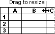
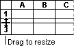
You can utilize this method by placing your mouse cursor on the line that separates your column or row heading from the one either to the right of or below it. For example, in the image below, I have placed my cursor on the line between columns B and C, because I want to automatically resize column B.

double click cell divider to resize a cell

Double-click this line to have Excel automatically adjust the size of your row or column.

Note that both of these methods will work if you want to resize multiple rows or columns at once, too. Simply hold down the Ctrl or Select key on your keyboard to select all of the rows or columns that you want to resize, then use the Row Height, Column Width or double-click method to adjust the size values of the selected cells.

Our guide on how to autofit all columns in Excel can show you a simple way to fix the width of your spreadsheet columns.

Matthew Burleigh has been writing tech tutorials since 2008. His writing has appeared on dozens of different websites and been read over 50 million times.

After receiving his Bachelor’s and Master’s degrees in Computer Science he spent several years working in IT management for small businesses. However, he now works full time writing content online and creating websites.

His main writing topics include iPhones, Microsoft Office, Google Apps, Android, and Photoshop, but he has also written about many other tech topics as well.

Read his full bio here.

Источник

Download Article

Using a Computer

Using the Mobile App

Do you have data in your spreadsheet that doesn’t fit into cells nicely? This wikiHow will teach you how to drag row and column boundaries to adjust cell size in Microsoft Excel.

1
Open your spreadsheet in Excel or create a new file. You can either open the saved spreadsheet within Excel by clicking File > Open, or you can right-click the file in your file explorer or Finder.
- This will work for Windows and Mac computers as well as the web version.^[1]
2

Move your cursor to the column or row heading that you want to adjust. You won’t be able to adjust a single cell inside a row or column, but you can change the size of the entire row’s cells.^[2]

Advertisement
3
Drag the boundary below the row heading (rows) or the boundary to the right (columns). As you drag the line down (rows) or right (columns), the cell size will increase. As you drag the line up (rows) or to the left (columns), the cell size will decrease.
- To select multiple rows or columns, press and hold Ctrl (PC) or ⌘ Cmd (macOS) as you click rows or columns.
- If you want the column or row to adjust automatically according to its contents, double-click the right boundary (for columns) or the bottom boundary (for rows).^[3]
- If you can’t drag the boundary, you need to check that drag-and-drop is enabled. To do that, go to File > Options. If you’re using Excel 2007, click the Microsoft Office Button icon (in the top left corner of the program) and then click Excel Options. Go to the «Advanced» category and select Enable fill handle and cell drag-and-drop then click Ok.^[4]

1

Open Excel. This app icon looks like a green square with a white «x» in front of another green rectangle that you can find on one of your Home screens, in the app drawer, or by searching.
2

Open your project or start a new one. When you open the app, you’ll see your OneDrive that lists all your current Excel projects, or you can tap the «New Project» icon to start a blank spreadsheet.
3

Tap the row or column heading you want to adjust. You should see two handle icons that you can drag and drop.
4

Drag and drop the handles to adjust row and column sizes. Remember that you have to tap the heading in order to get these handles. If you tap on a cell, you’ll just select the cell.^[5]

Ask a Question

200 characters left

Include your email address to get a message when this question is answered.

Submit

Thanks for submitting a tip for review!

References

About This Article

Article SummaryX

1. Open Excel.

2. Open your project or start a new one.

3. Tap the row or column heading you want to adjust.

4. Drag and drop the handles to adjust row and column sizes.

Did this summary help you?

Thanks to all authors for creating a page that has been read 30,380 times.

Is this article up to date?

Источник

See all How-To Articles

This tutorial demonstrates how to change cell size in pixels or inches in Excel and Google Sheets.

Change Ruler Units From Pixels to Inches

Sometimes you’ll need to change cells’ sizes in inches – rather than pixels – to accurately match your data or template. One way to do that is to use the Format feature.

To change the ruler units from the default to inches, in the Ribbon go to Files and click on the Options.

The Excel Options window opens. (1) From the right-side menu, choose Advanced and then on the left, scroll to the Display section. In it, (2) click on the box next to Ruler units and from the list, (3) choose Inches. (4) Click OK.

Change Cell Size by Formatting

Whether you’re using pixels or inches, changing a cell’s size works the same way

In the Ribbon, go to View > Page Layout.

To change the cell width, select the cells you want to resize, and then in the Ribbon go to Home > Format > Column Width.

In the Column width box, enter the new size in inches (here, 1.5 inches) and click OK.

This changes the width of the cell.

To change the height of the cells, select the cells you want to resize, and then in the Ribbon go to Home > Format > Row Height.

In the Row height box, enter the new size in inches (here, 1 inch) and press OK.

This changes the height of the cells.

Change Cell Size by Dragging

Another way to change cells sizes in inches or pixels is by dragging.

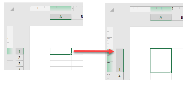
Change the view from Normal to Page Layout. In the Ribbon go to View > Page Layout.

To change the width of the cells, just place the cursor on the boundary on the right side of the column heading, When it changes to a double-headed arrow, drag it to the right to widen the cells or to the left to narrow them. You can see the width of selected cells in inches and pixels displayed in the box above the double-headed arrow. It allows you to measure exactly how much you want to change the width of the cells.

This changes the width of the cell.

To change the height of the cells, place the cursor on the boundary on the bottom side of the row heading. When the cursor changes to a double-headed arrow, just drag it up to make cells shorter or drag it down to make cells taller. While dragging, a similar box displays the height of the selected cells in inches and pixels, so you can measure exactly how much you want to change the height of the cells.

This changes the height of the cell.

Change Back to Default Size

Cell Height

In Excel, the default cell height is 15. To change back to that height, follow these steps:

To change back to default cell height, in the Ribbon go to View > Normal.

Then, select the cells whose height you want to change back to the default size, then in the Ribbon, go to Home > Format > Row Height.

In the Row height box enter 15 and click OK.

After that, the height of the selected cells goes back to the default size.

Cell Width

In Excel, the default cell width is 8.43. To change the cell width back to the default, follow these steps:

First, select the cells whose widths you want to change back to their default size, and then in the Ribbon, go to Home > Format > Column Width.

In the Column width box enter 8.43 and click OK.

As a result, the width of the selected cells goes back to the default size.

Note: You can use VBA code to revert to default cell sizes in Excel.

Change Cell Size in Google Sheets

To change the height and width of cells in the Google Sheets, follow these steps:

To change the width of cells, select the column you want to resize, right-click it, and from the drop-down list, choose Resize column.

In the dialog box, enter the new width (here, 200 pixels) in pixels and press OK.

As a result, the width of the column changes.

To change cell height, select the row you want to resize, right-click it, and from the list, choose Resize row.

In the dialog box, enter the height in pixels(here, 50 pixels) and click OK.

This changes the cells’ height.

Change to Default Cell Size in Google Sheets

In Google Sheets, the default cell width is 100 pixels, and the default cell height is 21 pixels.

To change back to the default cell width, first select the column you want to resize, right-click it, and from the list, choose Resize column.