Which one of the following options cannot be used in an excel spreadsheet formula

• 1. 

  Which do you press to enter the current date in a cell?

  • A. 

    CTRL+SHIFT+: (colon)

  • B. 

    CTRL+; (semicolon)

  • C. 

    CTRL+F10

• 2. 

  
  

  A fast way to add up this column of numbers is to click in the cell below the numbers and then:
   

  • A. 

    Click Subtotals on the Data menu.

  • B. 

    View the sum in the formula bar.

  • C. 

    Click the AutoSum button on the Standard toolbar, then press ENTER.

• 3. 

  
  

  How do you change column width to fit the contents?

  • A. 

    Single-click the boundary to the left of the column heading.

  • B. 

    Double-click the boundary to the right of the column heading.

  • C. 

    Press ALT and single-click anywhere in the column.

• 4. 

  Which of these is a quick way to copy formatting from a selected cell to two other cells on the same worksheet?

  • A. 

    Use CTRL to select all three cells, then click the Paste button on the Standard toolbar

  • B. 

    Copy the selected cell, then select the other two cells, click Style on the Format menu, then click Modify

  • C. 

    Click Format Painter on the Formatting toolbar twice, then click in each cell you want to copy the formatting to.

• 5. 

  
  

  What’s a quick way to extend these numbers to a longer sequence, for instance 1 through 20?

  • A. 

    Select both cells, and then drag the fill handle over the range you want, for instance 18 more rows.

  • B. 

    Select the range you want, including both cells, point to Fill on the Edit menu, and then click Down.

  • C. 

    Copy the second cell, click in the cell below it, on the Standard toolbar click the down arrow on the Paste button, and then click Paste Special.

• 6. 

  In order to save a new document in Microsoft Excel you must select which one of the following tool bar options?

  • A. 

    Edit

  • B. 

    Format

  • C. 

    Help

  • D. 

    File

• 7. 

  An Excel spreadsheet is primarily used for calculating which of the following options?

  • A. 

    Data

  • B. 

    Finances

  • C. 

    Numbers

  • D. 

    All of the above

• 8. 

  Which of the following option is a formula?

  • A. 

    =SUM(A1:A5)

  • B. 

    Add A1 — A5

  • C. 

    Subtract the numbers from A1 to A5

  • D. 

    A1 = A5

• 9. 

  Which one of the following options CANNOT be used in an Excel spreadsheet formula?

  • A. 

    = (equal sign)

  • B. 

    , (comma)

  • C. 

    & (ampersand)

  • D. 

    : (colon)

• 10. 

  What is the function of the word ‘=SUM’ at the beginning of an Excel spreadsheet formula?

  • A. 

    To add all the data together using addition only

  • B. 

    To tell the person viewing that this is a function and it should be added together

  • C. 

    To calculate all the data correctly without any mistakes

  • D. 

    To inform the computer that an arithmetic function will occur

• 11. 

  Which of the following INCORRECTLY selects multiple cells?

  • A. 

    (A1:G50)

  • B. 

    (A1, B3:C9)

  • C. 

    (A1:B5:C5)

  • D. 

    (A1:B5#C5)

Microsoft Excel has been one of the most valuable tools since the dawn of modern computing. Over a million people use Microsoft Excel spreadsheets daily to manage projects, track finances, create charts and graphs, and even manage time.

Unlike other applications such as Word, the spreadsheet software uses mathematical formulas and data in cells to calculate values.

However, there are instances when the Excel formulas do not function properly. This article will help you fix problems with Excel formulas.

1. Calculation Options Set to Manual

If you can’t update the value you’ve entered, and it returns the same as you entered, Excel’s calculation option may be set to manual and not automatic.

To fix this, change the calculation mode from Manual to Automatic.

1. Open the spreadsheet you’re having trouble with.
2. Then from the ribbon, navigate to the Formulas tab, then choose Calculation.
3. Select Calculation Options and choose Automatic from the dropdown.

Alternatively, you can adjust the calculation options from Excel options.

Choose the Office button at the top left corner > Excel options > Formulas > Workbook Calculation > Automatic. If you often switch between these two modes, you can create a custom keyboard shortcut for Excel to speed up your work.

2. Cell Is Formatted as Text

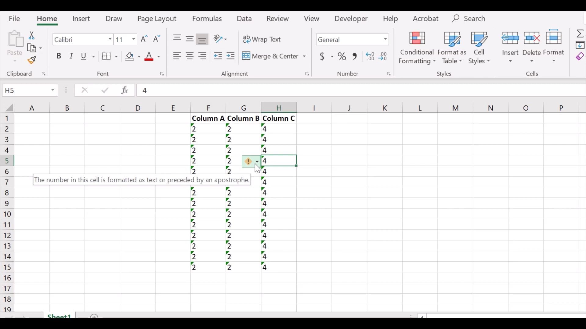
You might have accidentally formatted the cells containing the formulas as text. Unfortunately, Excel skips the applied formula when set to text format and displays the plain result instead.

The best way to check for formatting is to click on the cell and check the Number group from the Home tab. If it displays «Text,» click on that and choose General. To recalculate the formula, double-click the cell and press Enter on your keyboard.

3. Show Formulas Button Is Turned On

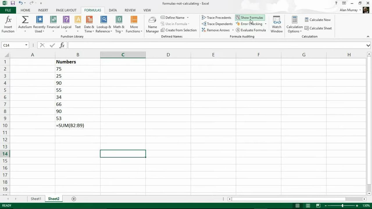
People commonly misuse the Show Formulas button by accidentally turning it on. With this turned on, the applied formulas will not work. You can find this setting under the Formulas tab.

The Show Formulas button is designed for auditing formulas, displaying the formula instead of the result when pressed. This might be a good tool if you want to better understand Excel formulas, but it stops them from working. In this case, turning it off may help resolve the issue.

Go to the Formulas tab > Formula Auditing Group and click the Show Formulas button.

4. Check Your Excel Formula

Even if you’re using an Excel function for beginners, a missing or an extra character might be why your Excel formula isn’t working. For example, when you enter an additional equal to (‘=’) or apostrophe (‘) in a spreadsheet cell, calculations are not performed, causing problems for users. The issue typically occurs when users try to copy a formula from the web.

However, it is simple to fix this problem. Just head over to the cell, select it, and remove the apostrophe or space at the beginning of the formula.

The same goes for the formula’s parentheses. When writing a lengthy formula, make sure you match all parentheses, so the calculations take place in the correct order. Excel helps you by showing parentheses pairs in different colors, so you can easily follow them.

Excel will display an error message when there’s a missing or extra parenthesis.

5. Use Proper Characters to Separate Arguments

You might have to separate function arguments to get the desired outcome depending on which Excel formulas you’re using. You should generally separate arguments using commas, but this may vary depending on your Regional Settings.

For example, in North American countries, you must enter commas to separate arguments, while in Europe, the right character is set to a semicolon. If you’ve used the wrong separating character, Excel might show the «We found a problem with this formula» error. You can try both options and check which one works for you.

If you’re used to using commas instead of semicolons, or vice versa, you can edit Excel settings to avoid repeating the same error.

1. Open Excel’s File menu and go to More > Options.
2. From the left pane, select Language.
3. In the Office display language section, click the Add a language button.
4. Select the wanted language to install and click Install.
5. Select it again and click Set as Preferred.
6. Test if Excel formulas are now working.

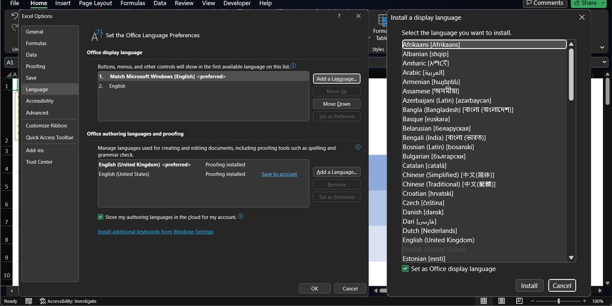
To sync Office settings across your devices when logging in with your Microsoft account, check the Store my authoring languages in the cloud for my account option.

6. Force Excel to Recalculate

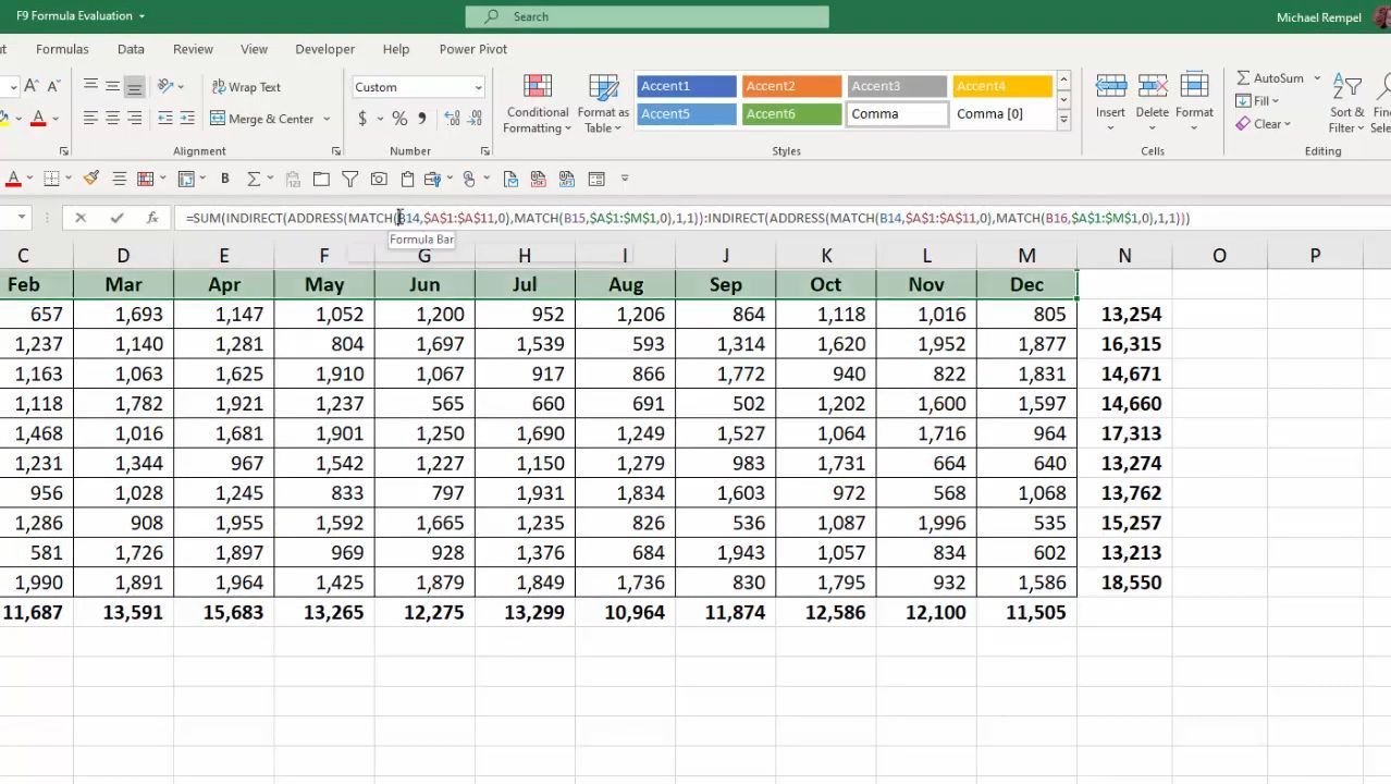
Excel allows users to recalculate formulas manually if they prefer not to use automatic calculation settings. You can do this with these methods:

For recalculating an entire spreadsheet, press F9 on your keyboard or choose Calculate Now under Formula Tab. Alternatively, you can recalculate an active sheet by pressing Shift + F9 on your keyboard or selecting Calculate Sheet from the Calculation group under Formula Tab.

You could also recalculate all formulas across all worksheets by pressing the Ctrl + Alt + F9 keyboard combination. Moreover, if you prefer recalculating just one formula from a sheet, select the cell and press Enter.

7. Check for Circular References

Excel formulas might show the wrong results if it uses circular referencing, which refers to the same cell where it does the calculations. Most of the time, Excel will notify you about a circular reference, but it might not do it every time.

Fortunately, you can manually check for this type of reference if you keep getting wrong results out of Excel formulas.

Open the Formulas tab, go to Formula Auditing, and select Error Checking > Circular References. Excel will show which cells have added a circular reference to the formula.

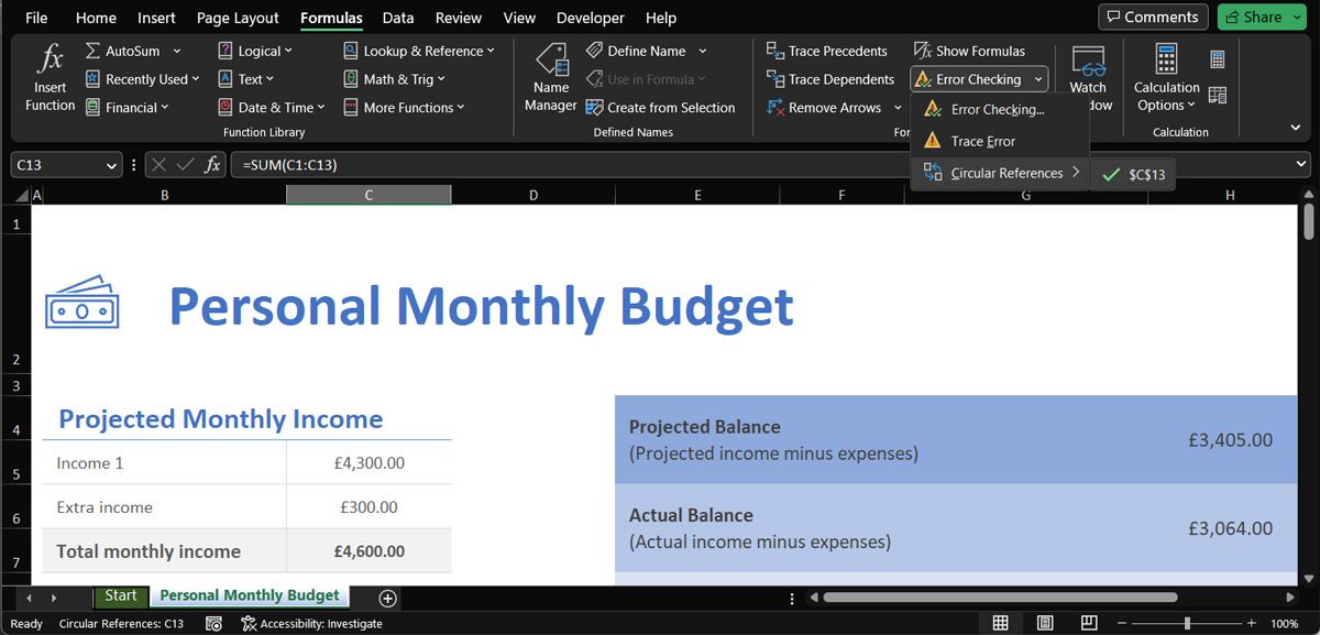
Go to the indicated cells and edit the formula so it doesn’t include the cell showing the results. For example, if the C13 cell shows the result for =SUM(C1:C13), change C13 to C12 within the formula to fix it.

Solve Your Excel Issues With These Fixes

The truth is, there’s not much room for error when writing an Excel formula. A missing parenthesis or the wrong cell format is enough to stop Excel formulas from working as intended.

However, you should know how to fix the issue as you’ll save a lot of time having Excel do the calculations for you.

Bottom Line: Learn about the different calculation modes in Excel and what to do if your formulas are not calculating when you edit dependent cells.

Skill Level: Beginner

Watch the Tutorial

Download the Excel File

You can follow along using the same workbook I use in the video. I’ve attached it below:

Why Aren’t My Formulas Calculating?

If you’ve ever been in a situation where the formulas in your spreadsheet are not automatically calculating as they should, you know how frustrating it can be.

This was happening to my friend Brett. He was telling me that he was working with a file and it wasn’t recalculating the formulas as he was entering data. He found that he had to edit each cell and hit Enter for the formula in the cell to update.

And it was only happening on his computer at home. His work computer was working just fine. This was driving him crazy and wasting a lot of time.

The most likely cause of this issue is the Calculation Option mode, and it’s a critical setting that every Excel user should know about.

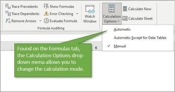
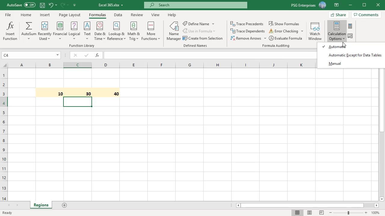
To check what calculation mode Excel is in, go to the Formulas tab, and click on Calculation Options. This will bring up a menu with three choices. The current mode will have a checkmark next to it. In the image below, you can see that Excel is in Manual Calculation Mode.

When Excel is in Manual Calculation mode, the formulas in your worksheet will not calculate automatically. You can quickly and easily fix your problem by changing the mode to Automatic. There are cases when you might want to use Manual Calc mode, and I explain more about that below.

Calculation Settings are Confusing!

It’s really important to know how the calculation mode can change. Technically, it’s is an application-level setting. That means that the setting will apply to all workbooks you have open on your computer.

As I mention in the video above, this was the issue with my friend Brett. Excel was in Manual calculation mode on his home computer and his files weren’t calculating. When he opened the same files on his work computer, they were calculating just fine because Excel was in Automatic calculation mode on that computer.

However, there is one major nuance here. The workbook (Excel file) also stores the last saved calculation setting and can change/override the application-level setting.

This should only happen for the first file you open during an Excel session.

For example, if you change Excel to manual calc mode before you save & close the file, then that setting is stored with the workbook. If you then open that workbook as the first workbook in your Excel session, the calculation mode will be changed to manual.

All subsequent workbooks that you open during that session will also be in manual calculation mode. If you save and close those files, the manual calc mode will be stored with the files as well.

The confusing part about this behavior is that it only happens for the first file you open in a session. Once you close the Excel application completely and then re-open it, Excel will return to automatic calculation mode if you start by opening a new blank file or any file that is in automatic calculation mode.

Therefore, the calculation mode of the first file you open in an Excel session dictates the calculation mode for all files opened in that session. If you change the calculation mode in one file, it will be changed for all open files.

Note: I misspoke about this in the video when I said that the calculation setting doesn’t travel with the workbook, and I will update the video.

The 3 Calculation Options

There are three calculation options in Excel.

Automatic Calculation means that Excel will recalculate all dependent formulas when a cell value or formula is changed.

Manual Calculation means that Excel will only recalculate when you force it to. This can be with a button press or keyboard shortcut. You can also recalculate a single cell by editing the cell and pressing Enter.

Automatic Except for Data Tables means that Excel will recalculate automatically for all cells except those that are used in Data Tables. This is not referring to normal Excel Tables that you might work with frequently. This refers to a scenario-analysis tool that not many people use. You find it on the Data tab, under the What-If Scenarios button. So unless you’re working with those Data Tables, it’s unlikely you will ever purposely change the setting to that option.

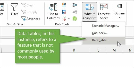
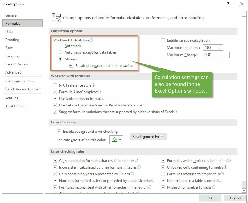
In addition to finding the Calculation setting on the Data tab, you can also find it on the Excel Options menu. Go to File, then Options, then Formulas to see the same setting options in the Excel Options window.

Under the Manual Option, you’ll see a checkbox for recalculating the workbook before saving, which is the default setting. That’s a good thing because you want your data to calculate correctly before you save the file and share it with your co-workers.

Why Would I Use Manual Calculation Mode?

If you are wondering why anyone would ever want to change the calculation from Automatic to Manual, there’s one major reason. When working with large files that are slow to calculate, the constant recalculation whenever changes are made can sometimes slow your system. Therefore people will sometimes switch to Manual mode while working through changes on worksheets that have a lot of data, and then will switch back.

When you are in Manual Calculation mode, you can force a calculation at any time using the Calculate Now button on the Formulas tab.

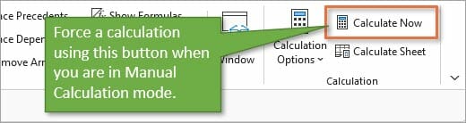
The keyboard shortcut for Calculate Now is F9, and it will calculate the entire workbook. If you want to calculate just the current worksheet, you can choose the button below it: Calculate Sheet. The keyboard shortcut for that choice is Shift + F9.

Here is a list of all Recalculate keyboard shortcuts:

Shortcut	Description
F9	Recalculate formulas that have changed since the last calculation, and formulas dependent on them, in all open workbooks. If a workbook is set for automatic recalculation, you do not need to press F9 for recalculation.
Shift+F9	Recalculate formulas that have changed since the last calculation, and formulas dependent on them, in the active worksheet.
Ctrl+Alt+F9	Recalculate all formulas in all open workbooks, regardless of whether they have changed since the last recalculation.
Ctrl+Shift+Alt+F9	Check dependent formulas, and then recalculate all formulas in all open workbooks, regardless of whether they have changed since the last recalculation.

Macro Changing to Manual Calculation Mode

If you find that your workbook is not automatically calculating, but you didn’t purposely change the mode, another reason that it may have changed is because of a macro.

Now I want to preface this by saying that the issue is NOT caused by all macros. It’s a specific line of code that a developer might use to help the macro run faster.

The following line of VBA code tells Excel to change to Manual Calculation mode.

Application.Calculation = xlCalculationManual

Sometimes the author of the macro will add that line at the beginning so that Excel does not attempt to calculate while the macro runs. The setting should then changed be changed back at the end of the macro with the following line.

Application.Calculation = xlCalculationAutomatic

This technique can work well for large workbooks that are slow to calculate.

However, the problem arises when the macro doesn’t get to finish—perhaps due to an error, program crash, or unexpected system issue. The macro changes the setting to Manual and it doesn’t get changed back.

As I mention in the video, this was exactly what happened to my friend Brett, and he was NOT aware of it. He was left in manual calc mode and didn’t know why, or how to get Excel calculating again.

Therefore, if you are using this technique with your macros, I encourage you to think about ways to mitigate this issue. And also warn your users of the potential of Excel being left in manual calc mode.

I also recommend NOT changing the Calculation property with code unless you absolutely need to. This will help prevent frustration and errors for the users of your macros.

Conclusion

I hope this information is helpful for you, especially if you are currently dealing with this particular issue. If you have any questions or comments about calculation modes, please share them in the comments.

If you work with formulas in Excel, sooner or later you will encounter the problem where Excel formulas don’t work at all (or give the wrong result).

While it would have been great had there been only a few possible reasons for malfunctioning formulas. Unfortunately, there are too many things that can go wrong (and often does).

But since we live in a world that follows the Pareto principle, if you check for some common issues, it’s likely to solve 80% (or maybe even 90% or 95% of the issues where formulas are not working in Excel).

And in this article, I will highlight those common issues that are likely the cause of your Excel formulas not working.

So let’s get started!

Incorrect Syntax of the Function

Let me start by pointing out the obvious.

Every function in Excel has a specific syntax – such as the number of arguments it can take or the type of arguments it can accept.

And in many cases, the reason your Excel formulas are not working or gives the wrong result could be an incorrect argument (or missing arguments).

For example, the VLOOKUP function takes three mandatory arguments and one optional argument.

If you provide a wrong argument or don’t specify the optional argument (where it’s needed for the formula to work), it’s going to give you a wrong result.

For example, suppose you have a dataset as shown below where you need to know the score of Mark in Exam 2 (in cell F2).

If I use the below formula, I will get the wrong result, because I am using the wrong value in the third argument (one that asks for Column Index number).

=VLOOKUP(A2,A2:C6,2,FALSE)

In this case, the formula calculates (as it returns a value), but the result is incorrect (instead of score in Exam 2, it gives the score in Exam 1).

Another example where you need to be cautious about the arguments is when using VLOOKUP with the approximate match.

Since you need to use an optional argument to specify where you want VLOOKUP to do an exact match or an approximate match, not specifying this (or using the wrong argument) can cause issues.

Below is an example where I have the marks data for some students and I want to extract marks in Exam 1 for the students in the table on the right.

When I use the below VLOOKUP formula it gives me an error for some names.

=VLOOKUP(E2,$A$2:$C$6,2)

This happens as I have not specified the last argument (which is used to determine whether to do an exact match or approximate match). When you don’t specify the last argument, it automatically does an approximate match by default.

Since we needed to do an exact match in this case, the formula returns an error for some names.

While I have taken the example of the VLOOKUP function, in this case, this is something that can be applicable for many Excel formulas that have optional arguments as well.

Also read: Identify Errors Using Excel Formula Debugging

Extra Spaces Causing Unexpected Results

Leading, trailing spaces are hard to find out and can cause issues when you use a cell that has these in formulas.

For example, in the below example, if I try to use VLOOKUP to fetch the score for Mark, it gives me the #N/A error (the not available error).

While I can see that the formula is correct and the name ‘Mark’ is clearly there is the list, what I can not see is that there is a trailing space in the cell that has the name (in cell D2).

Excel doesn’t consider the content of these two cells the same and therefore it considers it a mismatch when fetching the value using VLOOKUP (or it could be any other lookup formula).

To fix this issue, you need to remove these extra space characters.

You can do this by using any of the following methods:

1. Clean the cell and remove any leading/trailing spaces before using it in formulas
2. Use the TRIM function within the formula to make sure any leading/trailing/double spaces are ignored.

In the above example, you can use the below formula instead to make sure it works.

=VLOOKUP(TRIM(D2),$A$2:$B$6,2,0)

While I have taken the VLOOKUP example, this is also a common issue when working with TEXT functions.

For example, if I use the LEN function to count the total number of characters in a cell, if there are leading or trailing spaces, these would also be counted and give the wrong result.

Take away / How to Fix: If possible, clean your data by removing any leading/trailing or double spaces before using these in formulas. If you can not change the original data, use the TRIM function in formulas to take care of this.

Using Manual Calculation Instead of Automatic

This one setting can drive you crazy (if you don’t know it’s what’s causing all the issues).

Excel has two calculation modes – Automatic and Manual.

By default, the automatic mode is enabled, which means that in case I use a formula or make any changes in the existing formulas, it automatically (and instantly) makes the calculation and gives me the result.

This is the setting we are all used to.

In the automatic setting, whenever you make any change in the worksheet (such as entering a new formula to even some text in a cell), Excel automatically recalculates everything (yes, everything).

But in some cases, people enable the manual calculation setting.

This is mostly done when you have a heavy Excel file with a lot of data and formulas. In such cases, you may not want Excel to recalculate everything when you make small changes (as it may take a few seconds or even minutes) for this recalculation to complete.

If you enable manual calculation, Excel will not calculate unless you force it to.

And this may make you think that your formula is not calculating.

All you need to do in this case is either set the calculation back to automatic or force a recalculation by hitting the F9 key.

Below are the steps to change the calculation from manual to automatic:

1. Click the Formula tab
2. Click on Calculation Options
3. Select Automatic

Important: In case you’re changing the calculation from manual to automatic, it’s a good idea to create a backup of your workbook (just in case this makes your workbook hang or makes Excel crash)

Take away / How to Fix: If you notice that your formulas are not giving the expected result, try something simple in any cell (such as adding 1 to an existing formula. Once you identify the issue as the one where calculation mode needs to be changed, do a force calculation by using F9.

Deleting Rows/Column/Cells Leading to #REF! Error

One of the things that can have a devastating effect on your existing formulas in Excel is when you delete any row/column which has been used in calculations.

When this happens, sometimes, Excel adjusts the reference itself and makes sure that the formulas are working fine.

And sometimes… it can not.

Thankfully, one clear indication that you get when formulas break on deleting cells/rows/columns is the #REF! error in the cells. This is a reference error that tells you that there is some issue with the references in the formula.

Let me show you what I mean by using an example.

Below I have used the SUM formula to add the cells A2:A6.

Now, if I delete any of these cells/rows, the SUM formula will return a #REF! error. This happens because when I deleted the row, the formula doesn’t know what to reference now.

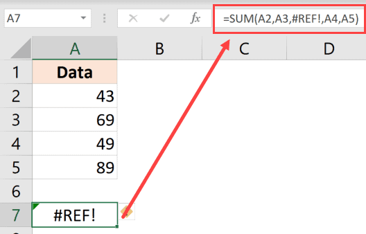
You can see that the third argument in the formula has become #REF! (which earlier referred to the cell that we deleted).

Take away / How to Fix: Before you delete any data that is being used in formulas, make sure there are no errors after the deletion. It’s also recommended that you create a backup of your work regularly to make sure you always have something to fall back on.

Incorrect Placement of Parenthesis (BODMAS)

As your formulas start to get bigger and more complex, it’s a good idea to use parenthesis to be absolutely clear of what part belongs together.

In some cases, you may have the parenthesis at the wrong place, which can either give you a wrong result or an error.

And in some cases, it’s recommended to uses parenthesis to make sure the formula understands what needs to be grouped and calculated first.

For example, suppose you have the following formula:

=5+10*50

In the above formula, the result is 505 as Excel first does the multiplication and then the addition (as there is an order of precedence when it comes to operators).

If you want it to first do the addition and then the multiplication, you need to use the below formula:

=(5+10)*50

In some cases, the order of precedence may work for you, but it’s still recommended that you use the parenthesis to avoid any confusion.

Also, in case you’re interested, below is the order of precedence for various operators often used in formulas:

Operator	Description	Order of Precedence
: (colon)	Range	1
(single space)	Intersection	2
, (comma)	union	3
–	Negation (as in –1)	4
%	Percentage	5
^	Exponentiation	6
* and /	Multiplication & division	7
+ and –	Addition & subtraction	8
&	Concatnenation	9
= < > <= >= <>	Comparison	10

Take away / How to Fix: Always use parenthesis to avoid any confusion, even if you know the order of precedence and are using it correctly. Having parenthesis makes it easier to audit formulas.

Incorrect Use of Absolute/Relative Cell References

When you copy and paste formulas in Excel, it automatically adjusts the references. Sometimes, this is exactly what you want (mostly when you’re copy-pasting formulas down the column), and sometimes you don’t want this to happen.

An absolute reference is when you fix a cell reference (or range reference) so that it doesn’t change when you copy and paste formulas, and a relative reference is one that changes.

You can read more about absolute, relative, and mixed references here.

You may get an incorrect result in case you forget to change the reference to an absolute one (or vice versa). This is something that happens quite often to me when I am using lookup formulas.

Let me show you an example.

Below I have a dataset where I want to fetch the score in Exam 1 for the names in column E (a simple VLOOKUP use case)

Below is the formula that I use in cell F2 and then copies to all the cells below it:

=VLOOKUP(E2,A2:B6,2,0)

As you can see that this formula gives an error in some cases.

This happens because I haven’t locked the table array argument – it’s A2:B6 in cell F2, while it should have been $A$2:$B$6

By having these dollar signs before the row number and column alphabet in a cell reference, I am forcing  Excel to keep these cell references fixed. So, even when I copy this formula down, the table array will continue to refer to A2:B6

Pro Tip: To convert a relative reference to an absolute one, select that cell reference within the cell, and press the F4 key. You would notice that it changes by adding the dollar signs. You can continue to press F4 until you get the reference you want.

Incorrect Reference to Sheet / Workbook Names

When you refer to other sheets or workbooks in a formula, you need to follow a specific format. And in case the format is incorrect, you will get an error.

For example, if I want to refer to cell A1 in Sheet2, the reference would be =Sheet2!A1 (where there is an exclamation sign after the sheet name)

And in case there are multiple words in the sheet name (let’s say it’s Example Data), the reference would be =’Example Data’!A1 (where the name is enclosed in single quotes followed by an exclamation sign).

In case you’re referring to an external workbook (let’s say you’re referring to cell A1 in ‘Example Sheet’ in the workbook named ‘Example Workbook’), the reference will be as shown below:

='[Example Workbook.xlsx]Example Sheet'!$A$1

And in case you close the workbook, the reference would change to include the entire path of the workbook (as shown below):

='C:UserssumitDesktop[Example Workbook.xlsx]Example Sheet'!$A$1

In case you end up changing the name of the workbook or the worksheet to which the formula refers to, it’s going to give you a #REF! error.

Also read: How to Find External Links and References in Excel

Circular References

A circular reference is when you refer (directly or indirectly) to the same cell where the formula is being calculated.

Below is a simple example, where I use the SUM formula in cell A4 while using it in the calculation itself.

=SUM(A1:A4)

Although Excel shows you a prompt letting you know about the circular reference, it will not do it for every instance. And this may give you the wrong result (without any warning).

In case you suspect circular reference in play, you can check which cells have it.

To do this, click the Formula tab and in the ‘Formula Auditing’ group, click on the Error Checking drop-down icon (the small downward pointing arrow).

Hover the cursor over the Circular reference option and it will show you the cell that has the circular reference issue.

Cells Formatted as Text

If you find yourself in a situation where as soon as you type the formula as hit enter, you see the formula instead of the value, it’s a clear case of the cell being formatted as text.

When a cell is formatted as text, it considers the formula as a text string and shows it as is.

It doesn’t force it to calculate and give the result.

And it has an easy fix.

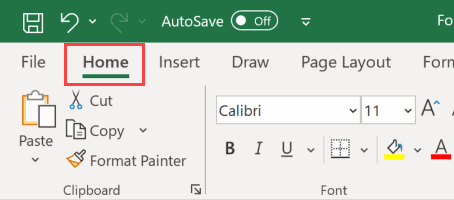
1. Change the format to ‘General’ from ‘Text’ (it’s in Home tab in the Numbers group)
2. Go to the cell that has the formula, get into the edit mode (use F2 or double click on the cell) and hit Enter

In case the above steps don’t solve the problem, another thing to check is whether the cell has an apostrophe at the beginning. A lot of people add an apostrophe to convert formulas and numbers to text.

If there is an apostrophe, you can simply remove it.

Text Automatically Getting Converted into Dates

Excel has this bad habit of converting that looks like a date into an actual date. For example, if you enter 1/1, Excel would convert it to 01-Jan of the current year.

In some cases, this may be exactly what you want, and in some cases, this may work against you.

And since Excel stores date and time values as numbers, as soon as you enter 1/1, it converts it into a number representing the January 1 of the current year. In my case, when I do this, it converts it into the number 43831 (for 01-01-2020).

This could mess with your formulas if you’re using these cells as an argument in a formula.

How to fix this?

Again, we don’t want Excel to automatically pick the format for us, so we need to clearly specify the format ourselves.

Below are the steps to change the format to text so that it doesn’t automatically convert text to dates:

1. Select the cells/range where you want to change the format
2. Click on the Home tab
3. In the Number group, click on the Format drop-down
4. Click on Text

Now, whenever you enter anything in the selected cells, it would be considered as text, and not changed automatically.

Note: The above steps would only work for data entered after the formatting has been changed. It will not change any text that has been converted to date before you made this formatting change.

Another example where this can be really frustrating is when you enter a text/number that has leading zeros. Excel automatically removes these leading zeros as it considers these useless. For example, if you enter 0001 in a cell, Excel will change it to 1. In case you want to keep these leading zeros, use the steps above.

Hidden Rows/Columns Can Give Unexpected Results

This is not a case of formula giving you the wrong result but of using the wrong formula.

For example, suppose you have a dataset as shown below and I want to get the sum of all the visible cells in column C.

In cell C12, I have used the SUM function to get the total sale value for all these given records.

So far so good!

Now, I apply a filter to the item column to only show the records for Printer sales.

And here is the problem – the formula in cell C12 still shows the same result – i.e., the sum of all the records.

As I said, the formula is not giving the wrong result. In fact, the SUM function is working just fine.

The issue is that we have used the wrong formula here.

SUM function can not account for the filtered data and give you the result for all the cells (hidden or visible). If you only want to get the sum/count/average of visible cells, use SUBTOTAL or AGGREGATE functions.

Key takeaway – Understand the correct use and limitations of a function in Excel.

These are some of the common causes that I have seen where your Excel formulas may not work or give unexpected or wrong results. I am sure there are many more reasons for an Excel formula to not work or update.

In case you know of any other reason (maybe something that irks you often), let me know in the comments section.

Hope you found this tutorial useful!

You may also like the following Excel tutorials:

• How to Lock Formulas in Excel
• How to Copy and Paste Formulas in Excel without Changing Cell References
• Show Formulas in Excel Instead of the Values
• Convert Text to Numbers in Excel
• Convert Date to Text in Excel
• Microsoft Excel Won’t Open; How to Fix it!
• Arrow Keys not Working in Excel | Moving Pages Instead of Cells
• 20 Advanced Excel Functions and Formulas