
horizontal.
The horizontal (category) axis, also known as the x axis, of a chart displays text labels instead of numeric intervals and provides fewer scaling options than are available for a vertical (value) axis, also known as the y axis, of the chart.
Contents
- 1 What is the x-axis used for?
- 2 Which column is x-axis in Excel?
- 3 What is an x-axis example?
- 4 How do you create an x-axis in Excel?
- 5 What information is on x-axis?
- 6 Is x-axis up or down?
- 7 How do you find the x and y-axis?
- 8 Do you say X or y-axis first?
- 9 What is the meaning of X coordinate?
- 10 What is the equation of x-axis?
- 11 How do I move the X-axis in Excel?
- 12 How do you add X-axis labels in Excel?
- 13 How do I change the X-axis scale in Excel?
- 14 Where is the x-axis on a bar graph?
- 15 What does the x-axis represent on a graph?
- 16 Where does the x-axis go?
- 17 Is X vertical or horizontal?
- 18 What is an X and Y coordinate?
What is the x-axis used for?
The line on a graph that runs horizontally (left-right) through zero. It is used as a reference line so you can measure from it.
Which column is x-axis in Excel?
Click “Edit” under the “Horizontal Axis Labels” list to open the “Axis Labels” dialog. Click the icon that displays a red arrow, and then highlight the column on the spreadsheet that you want to denote as the x-axis. In this example, this is all the numbers in column A.
What is an x-axis example?
X-axis is a horizontal axis. An example of an x-axis is the line across the bottom of a chart.The horizontal (H), or nearest horizontal, plane on a two- or three-dimensional grid, chart, or graph in a Cartesian coordinate system. See also Cartesian coordinates, y-axis, and z-axis.
How do you create an x-axis in Excel?
From the Design tab, Data group, select Select Data. In the dialog box under Horizontal (Category) Axis Labels, click Edit. In the Axis label range enter the cell references for the x-axis or use the mouse to select the range, click OK. Click OK.
What information is on x-axis?
The Axes. The independent variable belongs on the x-axis (horizontal line) of the graph and the dependent variable belongs on the y-axis (vertical line).
Is x-axis up or down?
The x-axis and y-axis are two lines that create the coordinate plane. The x-axis is a horizontal line and the y-axis is a vertical line.Reminder: the x-axis really runs left and right, and the y-axis runs up and down.
How do you find the x and y-axis?
Scientists like to say that the “independent” variable goes on the x-axis (the bottom, horizontal one) and the “dependent” variable goes on the y-axis (the left side, vertical one).
Do you say X or y-axis first?
The x-coordinate always comes first, followed by the y-coordinate.
What is the meaning of X coordinate?
Definition of x-coordinate
: a coordinate whose value is determined by measuring parallel to an x-axis specifically : abscissa.
What is the equation of x-axis?
The equation of the x-axis is x=0.
How do I move the X-axis in Excel?
Select the cluster column chart whose horizontal axis you will move, and click Kutools > Chart Tools > Move X-axis to Negative/Zero/Bottom.
How do you add X-axis labels in Excel?
Click the chart, and then click the Chart Layout tab. Under Labels, click Axis Titles, point to the axis that you want to add titles to, and then click the option that you want. Select the text in the Axis Title box, and then type an axis title.
How do I change the X-axis scale in Excel?
You can change the scale used by Excel by following these steps:
- Right-click on the axis whose scale you want to change. Excel displays a Context menu for the axis.
- Choose Format Axis from the Context menu.
- Make sure the Scale tab is selected.
- Adjust the scale settings, as desired.
- Click on OK.
Where is the x-axis on a bar graph?
The vertical axis of the bar graph is called the y-axis, while the bottom of a bar graph is called the x-axis.
What does the x-axis represent on a graph?
the horizontal line of figures along the bottom of a graph, often representing time: The x-axis represents expenditure and the y-axis profit.
Where does the x-axis go?
An x-axis is one of the axes of a two- or three-dimensional graph. The x-axis is the horizontal plane of a graph in a Cartesian coordinate system, which gives a numerical value to each point along the horizontal x-axis, as well as the vertical y-axis (in a two-dimensional graph).
Is X vertical or horizontal?
A horizontal line is a line extending from left to right. When you look at the sunrise over the horizon you are seeing the sunrise over a horizontal line. The x-axis is an example of a horizontal line.
What is an X and Y coordinate?
The x coordinate is a given number of pixels along the horizontal axis of a display starting from the pixel (pixel 0) on the extreme left of the screen. The y coordinate is a given number of pixels along the vertical axis of a display starting from the pixel (pixel 0) at the top of the screen.
Содержание
- Add or remove a secondary axis in a chart in Excel
- Add or remove a secondary axis in a chart in Office 2010
- Add a secondary axis
- Add an axis title for a secondary axis
- Need more help?
- Learn How to Show or Hide Chart Axes in Excel
- What to Know
- Hide and Display Chart Axes
- What Is an Axis?
- 3-D Chart Axes
- Vertical Axis
- Horizontal Axis
- Secondary Vertical Axis
- How To Plot X Vs Y Data Points In Excel
- Excel Plot X vs Y
- Add Axis Titles to X vs Y graph in Excel
- Add Data Labels to X and Y Plot
- Instant Connection to an Expert through our Excelchat Service
Add or remove a secondary axis in a chart in Excel
When the numbers in a chart vary widely from data series to data series, or when you have mixed types of data (price and volume), plot one or more data series on a secondary vertical (value) axis. The scale of the secondary vertical axis shows the values for the associated data series. A secondary axis works well in a chart that shows a combination of column and line charts. You can quickly show a chart like this by changing your chart to a combo chart.


Note: The following procedure applies to Office 2013 and newer versions. Looking for Office 2010 steps?
Select a chart to open Chart Tools.
Select Design > Change Chart Type.
Select Combo > Cluster Column — Line on Secondary Axis.
Select Secondary Axis for the data series you want to show.
Select the drop-down arrow and choose Line.
Add or remove a secondary axis in a chart in Office 2010
When the values in a 2-D chart vary widely from data series to data series, or when you have mixed types of data (for example, price and volume), you can plot one or more data series on a secondary vertical (value) axis. The scale of the secondary vertical axis reflects the values for the associated data series.
After you add a secondary vertical axis to a 2-D chart, you can also add a secondary horizontal (category) axis, which may be useful in an xy (scatter) chart or bubble chart.
To help distinguish the data series that are plotted on the secondary axis, you can change their chart type. For example, in a column chart, you could change the data series on the secondary axis to a line chart.
Important: To complete the following procedures, you must have an existing 2-D chart. Secondary axes are not supported in 3-D charts.
You can plot data on a secondary vertical axis one data series at a time. To plot more than one data series on the secondary vertical axis, repeat this procedure for each data series that you want to display on the secondary vertical axis.
In a chart, click the data series that you want to plot on a secondary vertical axis, or do the following to select the data series from a list of chart elements:
Click the chart.
This displays the Chart Tools, adding the Design, Layout, and Format tabs.
On the Format tab, in the Current Selection group, click the arrow in the Chart Elements box, and then click the data series that you want to plot along a secondary vertical axis.
On the Format tab, in the Current Selection group, click Format Selection.
The Format Data Series dialog box is displayed.
Note: If a different dialog box is displayed, repeat step 1 and make sure that you select a data series in the chart.
On the Series Options tab, under Plot Series On, click Secondary Axis and then click Close.
A secondary vertical axis is displayed in the chart.
To change the display of the secondary vertical axis, do the following:
On the Layout tab, in the Axes group, click Axes.
Click Secondary Vertical Axis, and then click the display option that you want.
To change the axis options of the secondary vertical axis, do the following:
Right-click the secondary vertical axis, and then click Format Axis.
Under Axis Options, select the options that you want to use.
To complete this procedure, you must have a chart that displays a secondary vertical axis. To add a secondary vertical axis, see Add a secondary vertical axis.
Click a chart that displays a secondary vertical axis.
This displays the Chart Tools, adding the Design, Layout, and Format tabs.
On the Layout tab, in the Axes group, click Axes.

Click Secondary Horizontal Axis, and then click the display option that you want.
In a chart, click the data series that you want to change.
This displays the Chart Tools, adding the Design, Layout, and Format tabs.
Tip: You can also right-click the data series, click Change Series Chart Type, and then continue with step 3.
On the Design tab, in the Type group, click Change Chart Type.
In the Change Chart Type dialog box, click a chart type that you want to use.
The first box shows a list of chart type categories, and the second box shows the available chart types for each chart type category. For more information about the chart types that you can use, see Available chart types.
Note: You can change the chart type of only one data series at a time. To change the chart type of more than one data series in the chart, repeat the steps of this procedure for each data series that you want to change.
Click the chart that displays the secondary axis that you want to remove.
This displays the Chart Tools, adding the Design, Layout, and Format tabs.
On the Layout tab, in the Axes group, click Axes, click Secondary Vertical Axis or Secondary Horizontal Axis, and then click None.
You can also click the secondary axis that you want to delete, and then press DELETE, or right-click the secondary axis, and then click Delete.
To remove secondary axes immediately after you add them, click Undo  on the Quick Access Toolbar, or press CTRL+Z.
When the values in a chart vary widely from data series to data series, you can plot one or more data series on a secondary axis. A secondary axis can also be used as part of a combination chart when you have mixed types of data (for example, price and volume) in the same chart.
In this chart, the primary vertical axis on the left is used for sales volumes, whereas the secondary vertical axis on the right side is for price figures.
Do any of the following:
Add a secondary axis
This step applies to Word for Mac only: On the View menu, click Print Layout.
In the chart, select the data series that you want to plot on a secondary axis, and then click Chart Design tab on the ribbon.
For example, in a line chart, click one of the lines in the chart, and all the data marker of that data series become selected.
Click Add Chart Element > Axes > and select between Secondary Horizontal or Second Vertical.
Add an axis title for a secondary axis
This step applies to Word for Mac only: On the View menu, click Print Layout.
In the chart, select the data series that you want to plot on a secondary axis, and then click Chart Design tab on the ribbon.
For example, in a line chart, click one of the lines in the chart, and all the data marker of that data series become selected.
Click Add Chart Element > Axis Titles > and select between Secondary Horizontal or Second Vertical.
Need more help?
You can always ask an expert in the Excel Tech Community, get support in the Answers community, or suggest a new feature or improvement. See How do I give feedback on Microsoft Office? to learn how to share your thoughts. We’re listening.
Источник
Learn How to Show or Hide Chart Axes in Excel
Tips to show, hide, and edit the three main axes in an Excel chart
What to Know
- Select a blank area of the chart to display the Chart Tools on the right side of the chart, then select Chart Elements (plus sign).
- To hide all axes, clear the Axes check box. To hide one or more axes, hover over Axes and select the arrow to see a list of axes.
- Clear the check boxes for the axes you want to hide. Select the check boxes for the axes you want to display.
This article explains how to display, hide, and edit the three main axes (X, Y, and Z) in an Excel chart. We’ll also explain more about chart axes in general. Instructions cover Excel 2019, 2016, 2013, 2010; Excel for Microsoft 365, and Excel for Mac.
Hide and Display Chart Axes
To hide one or more axes in an Excel chart:
Select a blank area of the chart to display the Chart Tools on the right side of the chart.
:max_bytes(150000):strip_icc()/Capture-5c7c58fac9e77c0001d19d5b.JPG)
Select Chart Elements, the plus sign (+), to open the Chart Elements menu.
:max_bytes(150000):strip_icc()/Capture-5c7c59cec9e77c00012f823d.JPG)
To hide all axes, clear the Axes check box.
:max_bytes(150000):strip_icc()/Capture-5c7c5a1146e0fb0001a5f05f.JPG)
To hide one or more axes, hover over Axes to display a right arrow.
Select the arrow to display a list of axes that can be displayed or hidden on the chart.
:max_bytes(150000):strip_icc()/Capture-5c7c5a3f46e0fb0001a5f060.JPG)
Clear the check box for the axes you want to hide.
Select the check boxes for the axes you want to display.
What Is an Axis?
An axis on a chart or graph in Excel or Google Sheets is a horizontal or vertical line containing units of measure. The axes border the plot area of column charts, bar graphs, line graphs, and other charts. An axis displays units of measure and provides a frame of reference for the data displayed in the chart. Most charts, such as column and line charts, have two axes that are used to measure and categorize data:
The vertical axis: The Y or value axis.
The horizontal axis: The X or category axis.
All chart axes are identified by an axis title that includes the units displayed in the axis. Bubble, radar, and pie charts are some chart types that do not use axes to display data.
3-D Chart Axes
In addition to horizontal and vertical axes, 3-D charts have a third axis. The z-axis, also called the secondary vertical axis or depth axis, plots data along the third dimension (the depth) of a chart.
Vertical Axis
The vertical y-axis is located along the left side of the plot area. The scale for this axis is usually based on the data values that are plotted in the chart.
Horizontal Axis
The horizontal x-axis is found at the bottom of the plot area, and contains category headings taken from the data in the worksheet.
Secondary Vertical Axis
A second vertical axis, which is found on the right side of a chart, displays two or more types of data in a single chart. It is also used to chart data values.
A climate graph or climatograph is an example of a combination chart that uses a second vertical axis to display both temperature and precipitation data versus time in a single chart.
Источник
How To Plot X Vs Y Data Points In Excel
We can use Excel to plot XY graph, also known as scatter chart or XY chart. With such charts, we can directly view trends and correlations between the two variables in our diagram. In this tutorial, we will learn how to plot the X vs. Y plots , add axis labels, data labels, and many other useful tips.
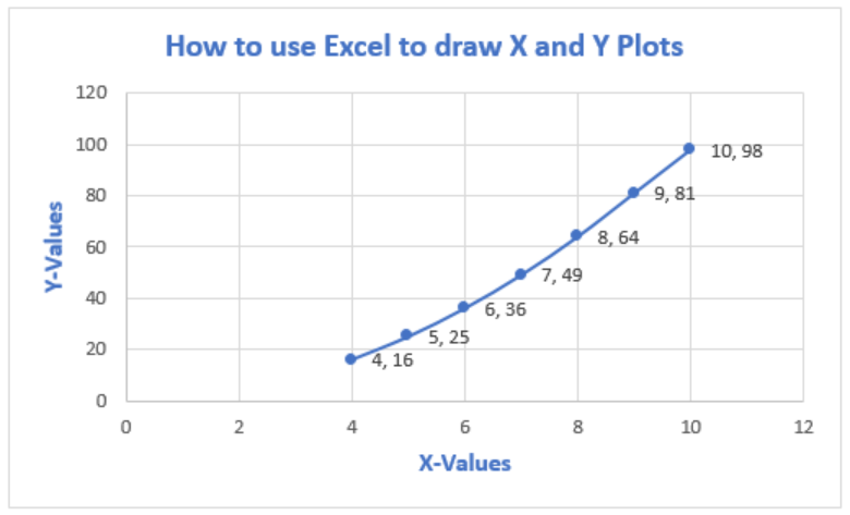 Figure 1 – How to plot data points in excel
Excel Plot X vs Y
We will set up a data table in Column A and B and then using the Scatter chart; we will display, modify, and format our X and Y plots.
- We will set up our data table as displayed below.
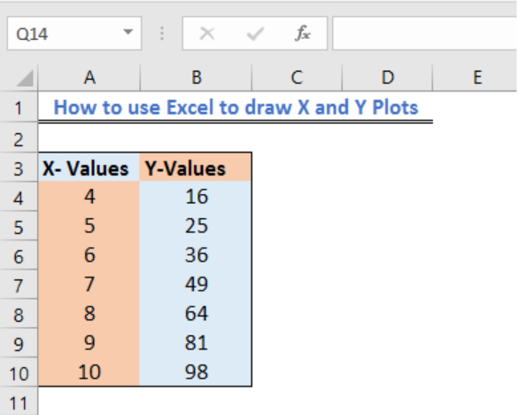 Figure 2 – Plotting in excel
- Next, we will highlight our data and go to the Insert Tab.
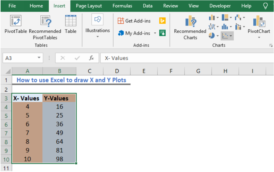 Figure 3 – X vs. Y graph in Excel
- If we are using Excel 2010 or earlier, we may look for the Scatter group under the Insert Tab
- In Excel 2013 and later, we will go to the Insert Tab ; we will go to the Charts group and select the X and Y Scatter chart. In the drop-down menu, we will choose the second option.
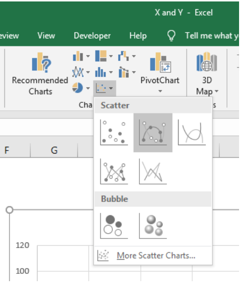 Figure 4 – How to plot points in excel
- Our Chart will look like this:
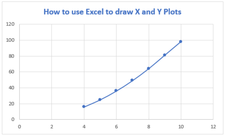 Figure 5 – How to plot x and y in Excel
Add Axis Titles to X vs Y graph in Excel
- If we wish to add other details to our graph such as titles to the horizontal axis, we can click on the Plot to activate the Chart Tools Tab. Here, we will go to Chart Elements and select Axis Title from the drop-down lists, which leads to yet another drop-down menu, where we can select the axis we want.
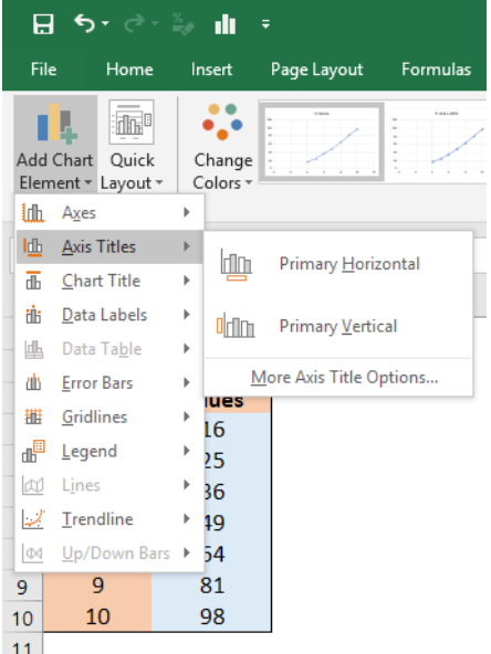 Figure 6 – Plot chart in Excel
- If we add Axis titles to the horizontal and vertical axis, we may have this
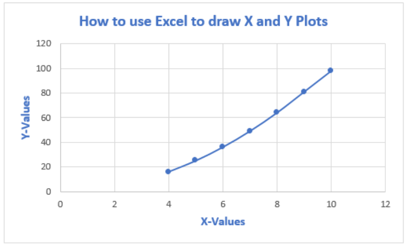 Figure 7 – Plotting in Excel
Add Data Labels to X and Y Plot
We can also add Data Labels to our plot. These data labels can give us a clear idea of each data point without having to reference our data table.
- We can click on the Plot to activate the Chart Tools Tab. We will go to Chart Elements and select Data Labels from the drop-down lists, which leads to yet another drop-down menu where we will choose More Data Table options
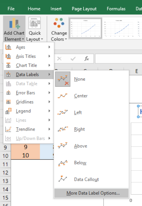 Figure 8 – How to plot points in excel
- In the Format Data Table dialog box, we will make sure that the X-Values and Y-Values are marked.
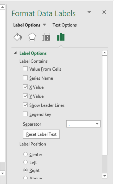 Figure 9 – How to plot x vs. graph in excel
- Our chart will look like this;
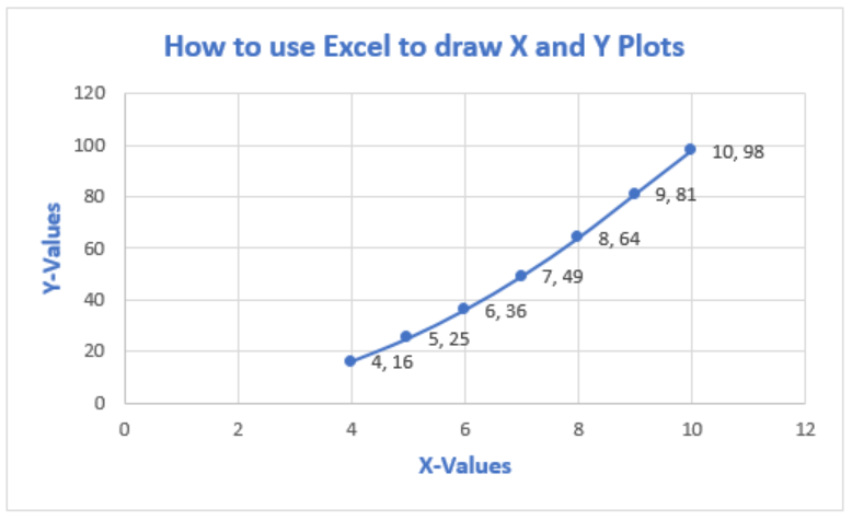 Figure 10 – Plot x vs. y in excel
- To Format Chart Axis , we can right click on the Plot and select Format Axis
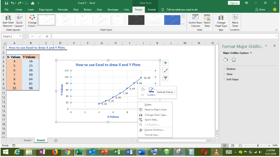 Figure 11 – Format Axis in excel x vs. y graph
- In the Format Axis dialog box , we can modify the minimum and maximum values.
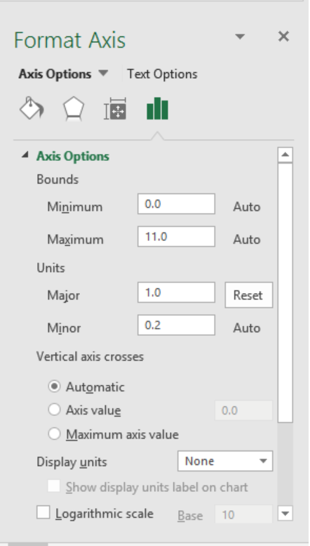 Figure 12 – How to plot x vs. y in excel
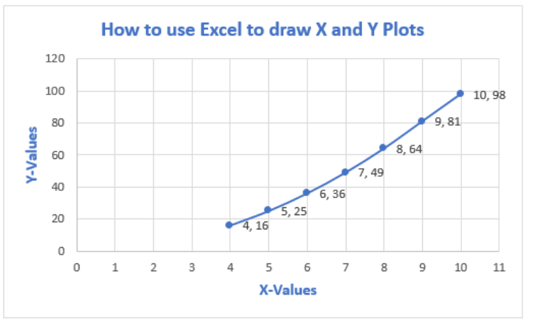 Figure 13 – How to plot data points in excel
Instant Connection to an Expert through our Excelchat Service
Most of the time, the problem you will need to solve will be more complex than a simple application of a formula or function. If you want to save hours of research and frustration, try our live Excelchat service! Our Excel Experts are available 24/7 to answer any Excel question you may have. We guarantee a connection within 30 seconds and a customized solution within 20 minutes.
Источник
Excel Chart Elements and Chart wizard
Many of our readers asking me to post tutorials to understand Excel Chart Elements and Chart wizard. This is the topic for those who wants to understand and getting started with excel charts. In this topic, We will see what are the different objects or elements related to charts, and how to access chart elements and change the chart properties. And then we will see what is the chart wizard in Excel what is the use of Chart Wizard in Excel.
- Charts in Excel
- Basic Elements of Excel Charts
- Basic Elements of Excel Charts – Chart Area
- Basic Elements of Excel Charts – Plot Area
- Basic Elements of Excel Charts – Chart Titles
- Basic Elements of Excel Charts – Chart Axis Titles
- Basic Elements of Excel Charts – Legends
- Basic Elements of Excel Charts – X-Axis
- Basic Elements of Excel Charts – Y-Axis
- Basic Elements of Excel Charts – Data Labels
- Basic Elements of Excel Charts – Gridlines
- Chart Wizard in Excel
There are many chart elements in excel to customize the charts to suit our data. Start learning Excel Chart Elements and Chart wizard to begin with Excel Charting.
Charts in Excel:
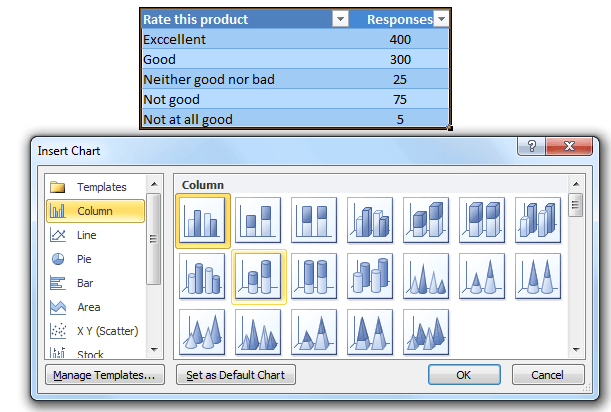
Charts help us to quickly understanding the data by plotting the data in graphs. We can present the data to visually represent with charts in Excel. Here is an example chart for customer ratings for an item. We can see the chart and quickly understand how the customers are liking a product.
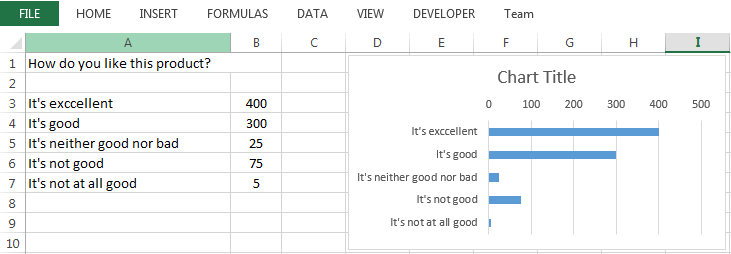
On left, we can see the data with customer satisfied. These are the responses for the questions “How do you like this product?”, There are 805 respondents answer this question and shared their opinion about an item on a 5 point rating scale.
On right, Chart is created with the customers responses. By looking the charts, we can quickly say that the customer satisfaction level is very good with the item. This is an example of Bar chart in Excel, which is suitable for quickly understanding the ranking data.
There are various types of the charts available in Excel to represent the data. We discuss this in Chart Types Tutorial.
Basic Elements of Excel Charts
The above chart is the basic charts in Excel, We can customize the charts by dealing with different Chart Element Objects and its properties. In this session we will focus on different elements of charts objects:
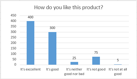
Here is an examples Column Chart for the same data shown above:
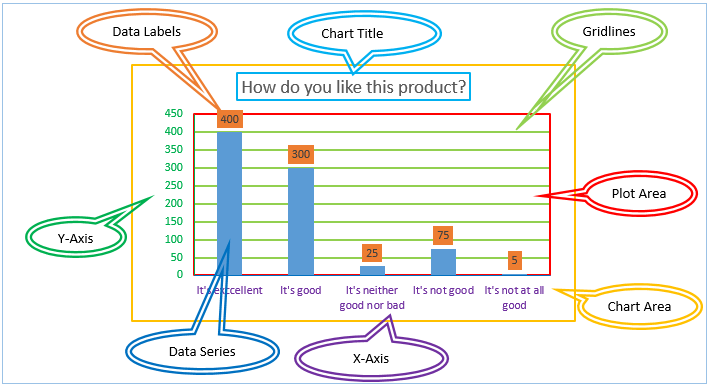
And here I have marked the basic chart elements in Excel each element with different clor for understanding purpose. Most of the times we generally deal with Chart Area, Plot Area, Chart Title, Legends, X-Axis, Y-Axis, Data Labels Data Series and Gridlines . Here is the pictorial representation of Chart Elements or Chart Objects in Excel:
Now will see each element of Excel Chart in detail:
Basic Elements of Excel Charts – Chart Area
Chart area in Excel Charts is the largest element (portion) of the Chart. We can format the Chart Area and change its border and background colors to make the charts looks more cleaner. Legends, Chart Titles and Plot Areas are the three major child elements of Chart Area.
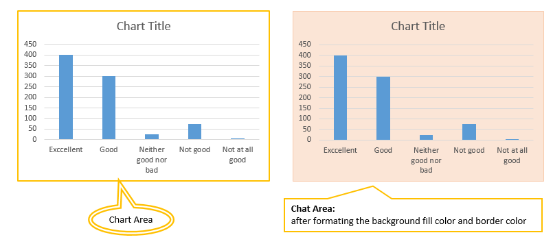
Generally we do not change the background color of the charts to make it look more professional. Charts looks more cleaner with white or default background color. However, we can change the background color to suite with the other parts of the excel sheets to make it consistent.
Basic Elements of Excel Charts – Plot Area
Plot Area is the second largest element (portion) in Excel Charts. It covers the actual chart data area. We can access the Plot Area and Format it to suit or needs.
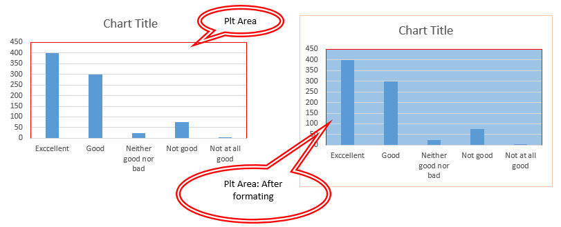
It is same as Chart Area, if your project need different background color then we change it. Otherwise default background color (white) looks more cleaner.
Basic Elements of Excel Charts – Chart Titles
We can provide the title in Excel Chart. There are three different chart titles we can provide in Excel charts, One Chart Title and Two Axis Titles.
Chart Title
Chart title is the main title of the chart, which is generally represents your chart and tell users what is this chart all about. Here is the Example Chart Tile we provided for the above Data.
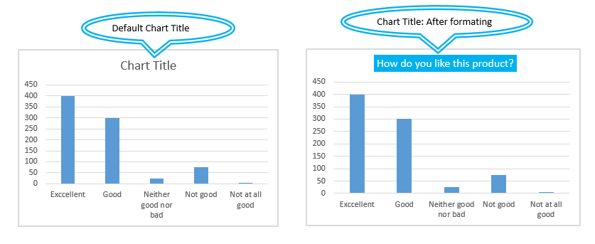
It is important to tell your user, What is this chart all about. So we generally provide the Chart titles, except some specific cases.
Basic Elements of Excel Charts – Chart Axis Titles
There are two Axis Titles which we can provide in Excel Charts. X-Axis title, which is for horizontal axis. and the second one is Y-Axis Titles, which is for Vertical Axis.
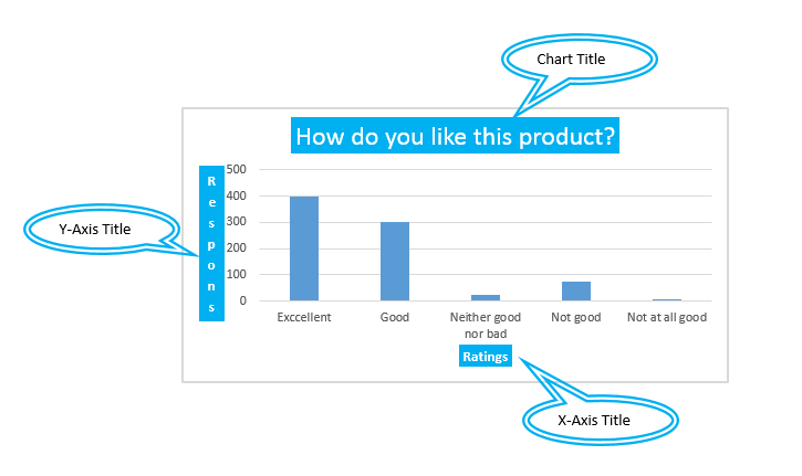
We should provide the chart Axes titles to make your users to understand the data and chart in better way. Most of the time, axis titles are shorter. However, some time we may need to provide longer titles to make it more clear.
Most of the times x-axis will have all your categories, so your x-axis title would be your category column name. And y-axis is your metric field, here you can mention the units in thousands, millions,etc.
Basic Elements of Excel Charts – Legends
When we have the data for more than one item, we need to distinguish between the data. We can take the advantage of the Chart Legend to show the difference between two categories.
Here is the example data and Chart with legends to understand the use of Chart Legends. Here we are showing the Overall satisfaction with Blue series and Quality in Orange Color. And Legends will help you to understand by providing the color definitions for each category of the data.
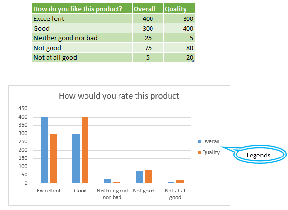
You can align the legends at any side of the Chart Area. If you have more number of category series, we generally place at right side of the chart plot area. Other wise we can place at top or bottom of the plot area to save the place.
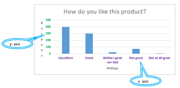
Basic Elements of Excel Charts – X-Axis
X-Axis in Excel Charts is the Horizontal Axis element in the chart. We generally plot the categories of our data on X-Axis. We can format x-axis as per our requirement. Make sure when we have longer category labels, we need to format chart axis to correctly fit the axis label into the chart
Basic Elements of Excel Charts – Y-Axis
Y-Axis in Excel Charts is the Vertical Axis element in the chart. It generally show the data range on Y-Axis. We can format x-axis as per our requirement. If we have two different types of data metrics, we can provide two y-axes, one is primary axis and the another one is secondary axis. Some times we may have large numbers in our data, in this case our chart looks more confusing. We can change the units to thosand, millions, etc. to make the charts more cleaner.
Basic Elements of Excel Charts – Data Labels
Data labels includes data values, category name, series name, legend keys and values form cells. We can choose all of these elements or any few as per our requirement.
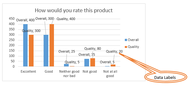
Data labels looks good when we have one or two data series. If you have more number of series, your chart looks confusing with overlapping data labels. Avoid data labels when you have more number of data series or consider changing the units into thousand, millions,etc.
Basic Elements of Excel Charts – Gridlines
Gridlines helps to quickly understand the values or percentage of the data without looking the exact values. we can understand the approximate value of the data by looking at the data series with gridlines.
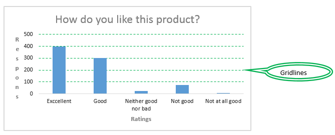
Again gridlines are sometime useful.You can delete the gridlines if they are not necessary to make your chart more cleaner.
Chart Wizard in Excel:
Excel Chart Wizard helps us to quickly to create charts in Excel. It is very easy to use and you can create rich visualized graphs in excel. You have to select the data first before launching the chart wizard.
Here is the Excel 2010 Chart wizard, it has number of charts to choose based on our data.
Here is the Excel 2013 Chart wizard, it more intelligent than Excel 2010. There are many charts provided to choose as per our data, and its provide recommended charts based on selected data.
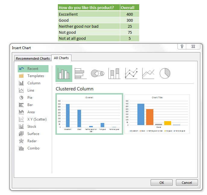
Ther are many options in Chart Wizard, we can create template with our frequently used charts. And also it will show you recently used charts to make our job more quicker. We can see the preview of the chart for the selected data in Excel 2013.
A Powerful & Multi-purpose Templates for project management. Now seamlessly manage your projects, tasks, meetings, presentations, teams, customers, stakeholders and time. This page describes all the amazing new features and options that come with our premium templates.
Save Up to 85% LIMITED TIME OFFER

All-in-One Pack
120+ Project Management Templates
Essential Pack
50+ Project Management Templates
Excel Pack
50+ Excel PM Templates
PowerPoint Pack
50+ Excel PM Templates
MS Word Pack
25+ Word PM Templates
Ultimate Project Management Template
Ultimate Resource Management Template
Project Portfolio Management Templates
Related Posts
- There are many chart elements in excel to customize the charts to suit our data. Start learning Excel Chart Elements and Chart wizard to begin with Excel Charting.
- Charts in Excel:
- Basic Elements of Excel Charts
- Chart Wizard in Excel:
VBA Reference
Effortlessly
Manage Your Projects
120+ Project Management Templates
Seamlessly manage your projects with our powerful & multi-purpose templates for project management.
120+ PM Templates Includes:
3 Comments
-
PRABHA MISHRA
May 29, 2015 at 10:10 AM — Replypls explain steps for all in details
-
S. Chowdhury
June 23, 2015 at 9:08 PM — ReplyI seek your kind cooperation to make a graph in excel with the undermentioned details. The x-axis should represent “Comprehensive”, “Individual”, “Group” and the YAxis should represent “Earned”, “Incurred” and “Expenses”
Comprehensive Individual Group
Earned 50000 40000 30000
Incurred 25000 15000 5000
Expenses 10000 8000 12000Your kind cooperation in this regard is sincerely solicited
Kindest regards
S. Chowdhury
-
nnothn
May 16, 2018 at 12:42 AM — Reply
Effectively Manage Your
Projects and Resources
ANALYSISTABS.COM provides free and premium project management tools, templates and dashboards for effectively managing the projects and analyzing the data.
We’re a crew of professionals expertise in Excel VBA, Business Analysis, Project Management. We’re Sharing our map to Project success with innovative tools, templates, tutorials and tips.
Project Management
Excel VBA
Download Free Excel 2007, 2010, 2013 Add-in for Creating Innovative Dashboards, Tools for Data Mining, Analysis, Visualization. Learn VBA for MS Excel, Word, PowerPoint, Access, Outlook to develop applications for retail, insurance, banking, finance, telecom, healthcare domains.
Page load link

3 Realtime VBA Projects
with Source Code!
Go to Top
Axis Type | Axis Titles | Axis Scale
Most chart types have two axes: a horizontal axis (or x-axis) and a vertical axis (or y-axis). This example teaches you how to change the axis type, add axis titles and how to change the scale of the vertical axis.
To create a column chart, execute the following steps.
1. Select the range A1:B7.

2. On the Insert tab, in the Charts group, click the Column symbol.

3. Click Clustered Column.

Result:

Axis Type
Excel also shows the dates between 8/24/2018 and 9/1/2018. To remove these dates, change the axis type from Date axis to Text axis.
1. Right click the horizontal axis, and then click Format Axis.

The Format Axis pane appears.
2. Click Text axis.

Result:

Axis Titles
To add a vertical axis title, execute the following steps.
1. Select the chart.
2. Click the + button on the right side of the chart, click the arrow next to Axis Titles and then click the check box next to Primary Vertical.

3. Enter a vertical axis title. For example, Visitors.
Result:

Axis Scale
By default, Excel automatically determines the values on the vertical axis. To change these values, execute the following steps.
1. Right click the vertical axis, and then click Format Axis.
The Format Axis pane appears.
2. Fix the maximum bound to 10000.
3. Fix the major unit to 2000.

Result:

Tips to show, hide, and edit the three main axes in an Excel chart
Updated on January 27, 2021
What to Know
- Select a blank area of the chart to display the Chart Tools on the right side of the chart, then select Chart Elements (plus sign).
- To hide all axes, clear the Axes check box. To hide one or more axes, hover over Axes and select the arrow to see a list of axes.
- Clear the check boxes for the axes you want to hide. Select the check boxes for the axes you want to display.
This article explains how to display, hide, and edit the three main axes (X, Y, and Z) in an Excel chart. We’ll also explain more about chart axes in general. Instructions cover Excel 2019, 2016, 2013, 2010; Excel for Microsoft 365, and Excel for Mac.
Hide and Display Chart Axes
To hide one or more axes in an Excel chart:
-
Select a blank area of the chart to display the Chart Tools on the right side of the chart.
-
Select Chart Elements, the plus sign (+), to open the Chart Elements menu.
-
To hide all axes, clear the Axes check box.
-
To hide one or more axes, hover over Axes to display a right arrow.
-
Select the arrow to display a list of axes that can be displayed or hidden on the chart.
-
Clear the check box for the axes you want to hide.
-
Select the check boxes for the axes you want to display.
What Is an Axis?
An axis on a chart or graph in Excel or Google Sheets is a horizontal or vertical line containing units of measure. The axes border the plot area of column charts, bar graphs, line graphs, and other charts. An axis displays units of measure and provides a frame of reference for the data displayed in the chart. Most charts, such as column and line charts, have two axes that are used to measure and categorize data:
The vertical axis: The Y or value axis.
The horizontal axis: The X or category axis.
All chart axes are identified by an axis title that includes the units displayed in the axis. Bubble, radar, and pie charts are some chart types that do not use axes to display data.
3-D Chart Axes
In addition to horizontal and vertical axes, 3-D charts have a third axis. The z-axis, also called the secondary vertical axis or depth axis, plots data along the third dimension (the depth) of a chart.
Vertical Axis
The vertical y-axis is located along the left side of the plot area. The scale for this axis is usually based on the data values that are plotted in the chart.
Horizontal Axis
The horizontal x-axis is found at the bottom of the plot area, and contains category headings taken from the data in the worksheet.
Secondary Vertical Axis
A second vertical axis, which is found on the right side of a chart, displays two or more types of data in a single chart. It is also used to chart data values.
A climate graph or climatograph is an example of a combination chart that uses a second vertical axis to display both temperature and precipitation data versus time in a single chart.
Thanks for letting us know!
Get the Latest Tech News Delivered Every Day
Subscribe