
Skip to content
![]()
Microsoft quietly replaced the comfortable Text Import Wizard from Excel and replaced it with the “Get & Transform” tools. The “Get & Transform” tools offer a lot of options and are very powerful. Unfortunately, they are quite complicated to use. Here is what you should now.
In a hurry? Click on “File” –> “Options” –> “Data” and set the corresponding checkmarks for reactivating the “Text Import Wizard” in Excel. Start the text import by clicking on “Data” –>”Get Data” –> “Legacy Wizards” –> “From Text (Legacy)”.
Introduction
In Excel 365 (only) 2016 (since version 1704) the “Text Import Wizard” was removed. It was replaced by the powerful “Get & Transform” tools. The “Get & Transform” tools also provide a function to import text and CSV files into Excel.
You have the following two options:
- Luckily, the comfortably “Text Import Wizard” still exists. You can re-activate and use it for importing text and csv files into Excel.
- Use the import function of the “Get & Transform” tools.
Restore the “Text Import Wizard”
The good news: You can easily restore the “Text Import Wizard”. Unfortunately, the option for re-activating them is hidden.
Follow these steps:
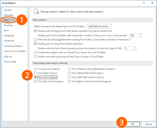
- Click on File and then on “Options”. Go to “Data” on the left-hand side.
- In the lower section of the window you can select the wizard you’d like to restore. For only importing text- or csv-files, select “From Text (Legacy)”. Feel free to also activate the corresponding wizard for importing Access files, files from web, from SQL servers and so on.
- Confirm with OK.
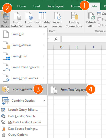
Now, you can find the so-called “Legacy Wizards” in the “Get Data” drop-down menu. In order to use them, follow these steps:
- Go to the “Data” ribbon.
- Click on “Get Data” on the left-hand side.
- Next, go to “Legacy Wizards”.
- Click on “From Text (Legacy)”.
How to use the “Text Import Wizard”
The steps for using the “Text Import Wizard” in Excel are shown in the screenshots.
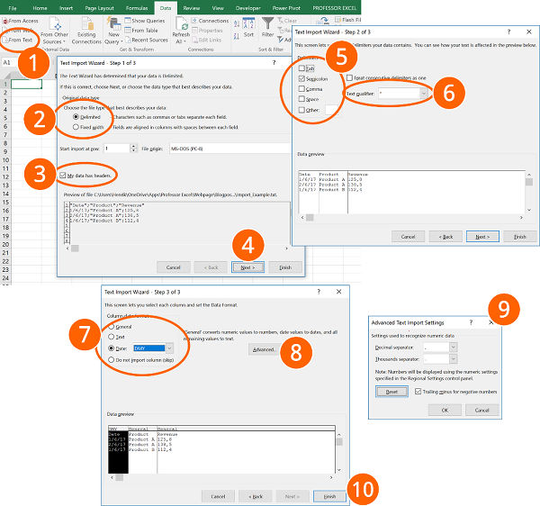
- Go to the “Data” ribbon and click on “From Text”. If you have a recent Excel version and there is no button called “From Text” (but instead “From Text/CSV”), click on “Get Data”, then on “Legacy Wizards” and then on “From Text (Legacy)”. Please refer to the paragraph above if this option is missing.
- Select how you want to define the columns: Either with a character as a separator or with a fixed width.
- If the first row contains headers, check the corresponding box.
- Continue with “Next >”.
- Select the delimiter. This is the character dividing the data into columns, for example “Tab”, “Semicolon” or “Comma”.
- Usually text fields use quotation marks marking the beginning and end of a text field.
- For each column, you can choose the data format. For dates, you could define the order of days, months and years.
- Click on “Advanced”…
- …for defining decimals and thousands separators.
- Finalize the import by clicking on “Finish”.
Import text and csv files with the “Get & Transform” tools
Importing text files in Excel with the “Get & Transform” tools requires many steps. Please refer to the numbers on the screenshots:
- Click on “From Text/CSV” on the “Data” ribbon in order to start the import process.
- Choose the delimiter (e.g. semi-colon, comma etc.). Here you can also switch to “Fixed Width”. If you want to separate your import data with the “Fixed Width” option, you have to type the numbers of characters, after which you want to data to be divided.
- For further options (e.g. switching thousands- and decimal separators) click on “Edit”.
- If you data is not represented correctly, delete the automatically created step “Changed Type”.
- Change the date format: Right-click on a column that contains a date. Alternatively click on the small “ABC” symbol in the top left corner of the column heading.
- Move the mouse to “Change Type”.
- Click on “Using Locale…”.
- Select “Date”.
- Select the locale format for dates. In this example, the German date format is used.
- Confirm with OK. Repeat the steps 5 to 10 for each date column.
Recommendation: Select several date columns at the same time by pressing and holding the Ctrl key while selecting the columns. - Change the decimal and thousand separators: Right-click again on a column with decimal numbers.
- Move the mouse to “Change Type”.
- Click on “Using Local…”.
- Choose “Decimal Number”.
- Select the local number format. Please refer to this article for a list of local number formats.
- Confirm with “OK”.
- Last step: Insert the data into a worksheet. In order to achieve this, click on “Close & Load” in the top-left corner.

Henrik Schiffner is a freelance business consultant and software developer. He lives and works in Hamburg, Germany. Besides being an Excel enthusiast he loves photography and sports.
We use cookies on our website to give you the most relevant experience by remembering your preferences and repeat visits. By clicking “Accept”, you consent to the use of ALL the cookies.
.
Chart Wizard in Excel is a wizard that takes users or guides them through a step-by-step process to insert a chart in an Excel spreadsheet. It was available in Excel in older versions under “Chart Wizard.” In addition, we have the “Recommended Charts” option for the newer versions, where Excel itself recommends various types of charts to choose from.
Table of contents
- Chart Wizard in Excel
- How to Build a Chart using the Excel Chart Wizard?
- Things to Remember
- Recommended Articles
You are free to use this image on your website, templates, etc, Please provide us with an attribution linkArticle Link to be Hyperlinked
For eg:
Source: Excel Chart Wizard (wallstreetmojo.com)
How to Build a Chart using the Excel Chart Wizard?
You can download this Chart Wizard Excel Template here – Chart Wizard Excel Template
Let us consider the below data as our chart data. Based on this data, we are going to build a chart.
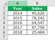
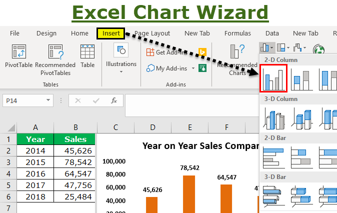
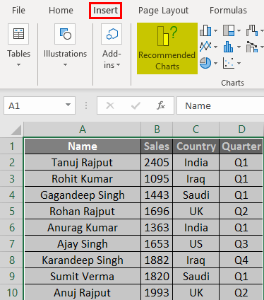
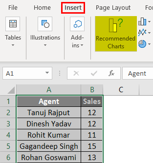
- Step 1: Firstly, we need to select the data first. In this case, the data range is A1 to B6.
- Step 2: We need to go to the “Insert” tab. Then, under the INSERT tabIn excel “INSERT” tab plays an important role in analyzing the data. Like all the other tabs in the ribbon INSERT tab offers its own features and tools. Under Insert Tab we have several other groups including tables, illustration, add-ins, charts, Power map, sparklines, filters, etc.read more, go to the “Charts” area.

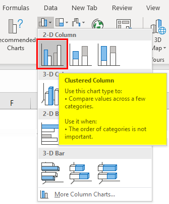
- Step 3: Since we have selected a column chart, click on the “Column Charts.”
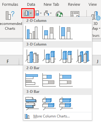
- Step 4: Select the first chart in this.
- Step 5: As soon as we click on this chart, Excel shows the default chart like the one below.
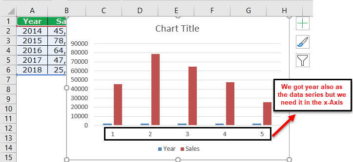
- Step 6: This is not a fully equipped chart. We need to make adjustments to this chart to look better and more beautiful.
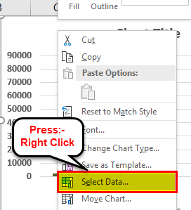
Firstly, right-click on the chart and select “Select Data.”
- Step 7: In the below window, we need only the “Sales” column to be shown as column bars, so we must remove “Year” from this list.
- Step 8: After removing it, we need “Year” to appear on the X-axis. So, we must click on the “Edit” button on the right-hand side.
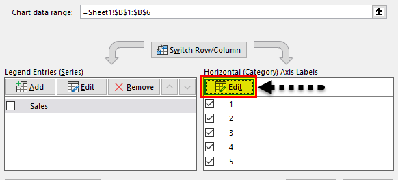
- Step 9: Now, select the “Year” range as the reference.
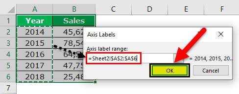
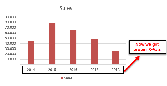
- Step 10: Click on “OK” to back to the previous window. Again, click on the “OK” button to complete the chart building. We have a chart ready now
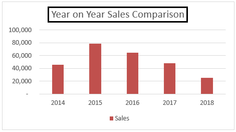
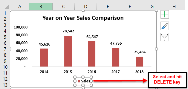
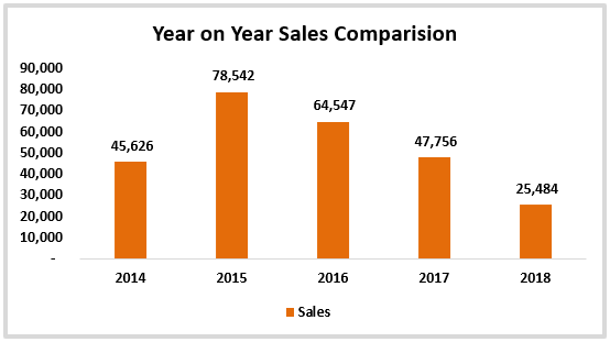
- Step 11: We need to change the chart’s name to “Year on Year Sales Comparison.” To change the chart title, double-click on the chart title and enter the chart title.
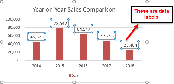
- Step 12: Add “Data Labels.” “Data Labels” are nothing but each data bar’s actual numbers. Let us show the data labels on each bar now.
Then, we need to right-click on one of the bars and select “Add Data Labels.”
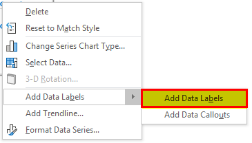
Now, we can see data labels for each label.
- Step 13: The next thing in the beautification process is removing gridlines. Gridlines in excelGridlines are little lines made of dots to divide cells from each other in a worksheet. The gridlines have slight faint invisibility; you can find it in the page layout tab. This option has a checkbox; for activating the gridlines, you can tick on it and untick if you wish to deactivate gridlines.read more are the tiny gray-colored line in the chart plot area.
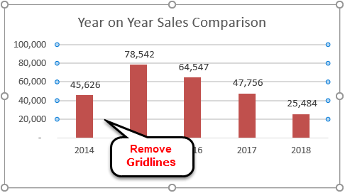
Select the gridline and press the “Delete” key to delete them. As a result, we will have a chart without gridlines.
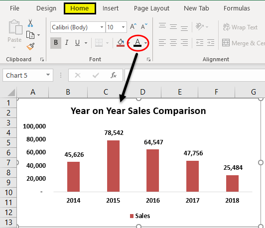
- Step 14: Change the color of the chart fonts to black. Select the chart and the black font color in the “Home” tab.
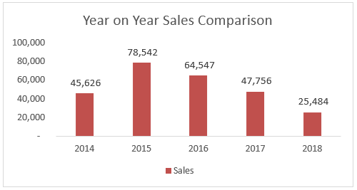
- Step 15: Since we have only one set of data in this chart, we need to remove the legend from the chartExcel chart legends depict description of significant elements and provides easy access to any chart. These legends are represented with the help of colours or symbols and distinguish data for better understanding.read more.
- Step 16: We can change the default column bar color to any of the colors as per our wish under the “Home” tab. Select the bar and choose the color of your choice.
Things to Remember
These are the processes involved in creating a chart. Below are some points to remember here.
- It will cover all the things you should know about excel chart creation. Up until Excel 2007, version Excel had its wizard tool, which would have guided the beginners in creating charts in Excel. But, from Excel 2007 versions, they eliminated “Chart Wizard” and integrated ribbon interface excelRibbons in Excel 2016 are designed to help you easily locate the command you want to use. Ribbons are organized into logical groups called Tabs, each of which has its own set of functions.read more, which is far better than the traditional “Chart Wizard.”
- Under “Select Data,” we can select and delete unwanted things.
- If Excel does not give you the proper X-axis, you need to follow Steps 8 and 9.
- We must show legends only in the case of two or more items. In the case of a single item, remove the legend.
Recommended Articles
This article has been a guide to Excel Chart Wizard. We discuss building an Excel chart wizard, practical examples, and a downloadable Excel template. You may learn more about Excel from the following articles: –
- Pie Chart in Excel
- Examples of Line Chart
- Chart Templates in Excel
- Dynamic Excel Chart
Now in Excel 365, we have the Get & Transform area available, which has been described in an older post of mine. The Get & Transform area of the Data tab on the ribbon is superior in terms of Data Connectors and Transformational capabilities. However though, sometimes we just want to use one of the old wizards to import our data such as the Legacy Wizards.

The Legacy Wizards do not appear in the Get & Transform area now, they are just hidden waiting for us to turn them on. Below you can find out How To Turn On The Legacy Wizards In Microsoft Excel 365.

We must select the File tab in order to move to Backstage View. Once in Backstage View, from the left of the drop down menu we select the category Options as shown in the image below.

Once we select the Option command, the Excel Options dialog box appears, where from the left once more, we select the category Data. Under this category we can Change Options Related To Data Import And Data Analysis, as shown below.

At the bottom part of the Data area we notice the area mentioning Show Legacy Data Import Wizards. All we need to do is to activate or deactivate the check boxes at the left of the commands that we need, and which will be displayed in Excel. The commands that are available are the following:
-
From Access
-
From Web
-
From Text
-
From SQL
-
From OData Data Feed
-
From XML Data Import
-
From Data Connection Wizard
Once we do all the adjustments that we need, we press the Ok button at the bottom right corner of the Excel Options dialog box, in order for us to return to Excel and for our adjustments to take place.

In the image below, I have activated all the Legacy Data Import Wizards, from the Excel Options dialog box, and then from the Data tab and from the left area of the ribbon named Get & Transform Data, we select the Get Data command as shown below and from Now, from the drop-down menu we notice the Legacy Wizards command, with all the available commands that we activated.

Below you can check out the video describing Turn On The Legacy Wizards In Microsoft Excel 365.
Don’t Forget To Subscribe To My YouTube Channel.


About Smart Office — philippospan
MVP:
Honored with the MVP (Most Valuable Professional) for OFFICE SYSTEM title for the years 2011, 2012, 2013, 2014 and 2015 by Microsoft, for my contribution and commitment to the technical communities worldwide.
Microsoft Master Specialist:
This certification provides skill-verification tools that not only help assess a person’s skills in using Microsoft Office programs but also the ability to quickly complete on-the-job tasks across multiple programs in the Microsoft Office system
Posted on June 18, 2018, in Excel 365 English, Microsoft Office 365 ProPlus English and tagged backstage view, Change Options Related To Data Import And Data Analysis, Data, Data Connectors, File, From Access, From Data Connection Wizard, From OData Data Feed, From SQL, From Text, From Web, From XML Data Import, Get & Transform, Legacy Data Import Wizards, Legacy Wizards, Microsoft Excel, Microsoft Office, Office Smart, Office System, Options, Smart Office, Subscribe, Turn On The Legacy Wizards In Microsoft Excel 365, YouTube. Bookmark the permalink. Comments Off on Turn On The Legacy Wizards In Microsoft Excel 365.
Excel for Microsoft 365 Excel 2021 Excel 2019 Excel 2016 Excel 2013 Excel 2010 Excel 2007 Excel Starter 2010 More…Less
Although you can’t export to Excel directly from a text file or Word document, you can use the Text Import Wizard in Excel to import data from a text file into a worksheet. The Text Import Wizard examines the text file that you are importing and helps you ensure that the data is imported in the way that you want.
Go to the Data tab > Get External Data > From Text. Then, in the Import Text File dialog box, double-click the text file that you want to import, and the Text Import Wizard dialog will open.
Step 1 of 3
Original data type If items in the text file are separated by tabs, colons, semicolons, spaces, or other characters, select Delimited. If all of the items in each column are the same length, select Fixed width.
Start import at row Type or select a row number to specify the first row of the data that you want to import.
File origin Select the character set that is used in the text file. In most cases, you can leave this setting at its default. If you know that the text file was created by using a different character set than the character set that you are using on your computer, you should change this setting to match that character set. For example, if your computer is set to use character set 1251 (Cyrillic, Windows), but you know that the file was produced by using character set 1252 (Western European, Windows), you should set File Origin to 1252.
Preview of file This box displays the text as it will appear when it is separated into columns on the worksheet.
Step 2 of 3 (Delimited data)
Delimiters Select the character that separates values in your text file. If the character is not listed, select the Other check box, and then type the character in the box that contains the cursor. These options are not available if your data type is Fixed width.
Treat consecutive delimiters as one Select this check box if your data contains a delimiter of more than one character between data fields or if your data contains multiple custom delimiters.
Text qualifier Select the character that encloses values in your text file. When Excel encounters the text qualifier character, all of the text that follows that character and precedes the next occurrence of that character is imported as one value, even if the text contains a delimiter character. For example, if the delimiter is a comma (,) and the text qualifier is a quotation mark («), «Dallas, Texas» is imported into one cell as Dallas, Texas. If no character or the apostrophe (‘) is specified as the text qualifier, «Dallas, Texas» is imported into two adjacent cells as «Dallas and Texas».
If the delimiter character occurs between text qualifiers, Excel omits the qualifiers in the imported value. If no delimiter character occurs between text qualifiers, Excel includes the qualifier character in the imported value. Hence, «Dallas Texas» (using the quotation mark text qualifier) is imported into one cell as «Dallas Texas».
Data preview Review the text in this box to verify that the text will be separated into columns on the worksheet as you want it.
Step 2 of 3 (Fixed width data)
Data preview Set field widths in this section. Click the preview window to set a column break, which is represented by a vertical line. Double-click a column break to remove it, or drag a column break to move it.
Step 3 of 3
Click the Advanced button to do one or more of the following:
-
Specify the type of decimal and thousands separators that are used in the text file. When the data is imported into Excel, the separators will match those that are specified for your location in Regional and Language Options or Regional Settings (Windows Control Panel).
-
Specify that one or more numeric values may contain a trailing minus sign.
Column data format Click the data format of the column that is selected in the Data preview section. If you do not want to import the selected column, click Do not import column (skip).
After you select a data format option for the selected column, the column heading under Data preview displays the format. If you select Date, select a date format in the Date box.
Choose the data format that closely matches the preview data so that Excel can convert the imported data correctly. For example:
-
To convert a column of all currency number characters to the Excel Currency format, select General.
-
To convert a column of all number characters to the Excel Text format, select Text.
-
To convert a column of all date characters, each date in the order of year, month, and day, to the Excel Date format, select Date, and then select the date type of YMD in the Date box.
Excel will import the column as General if the conversion could yield unintended results. For example:
-
If the column contains a mix of formats, such as alphabetical and numeric characters, Excel converts the column to General.
-
If, in a column of dates, each date is in the order of year, month, and date, and you select Date along with a date type of MDY, Excel converts the column to General format. A column that contains date characters must closely match an Excel built-in date or custom date formats.
If Excel does not convert a column to the format that you want, you can convert the data after you import it.
-
Convert numbers stored as text to numbers
-
Convert dates stored as text to dates
-
TEXT function
-
VALUE function
When you have selected the options you want, click Finish to open the Import Data dialog and choose where to place your data.
Import Data
Set these options to control how the data import process runs, including what data connection properties to use and what file and range to populate with the imported data.
-
The options under Select how you want to view this data in your workbook are only available if you have a Data Model prepared and select the option to add this import to that model (see the third item in this list).
-
Specify a target workbook:
-
If you choose Existing Worksheet, click a cell in the sheet to place the first cell of imported data, or click and drag to select a range.
-
Choose New Worksheet to import into a new worksheet (starting at cell A1)
-
-
If you have a Data Model in place, click Add this data to the Data Model to include this import in the model. For more information, see Create a Data Model in Excel.
Note that selecting this option unlocks the options under Select how you want to view this data in your workbook.
-
Click Properties to set any External Data Range properties you want. For more information, see Manage external data ranges and their properties.
-
Click OK when you’re ready to finish importing your data.
Notes: The Text Import Wizard is a legacy feature, which may need to be enabled. If you haven’t already done so, then:
-
Click File > Options > Data.
-
Under Show legacy data import wizards, select From Text (Legacy).
Once enabled, go to the Data tab > Get & Transform Data > Get Data > Legacy Wizards > From Text (Legacy). Then, in the Import Text File dialog box, double-click the text file that you want to import, and the Text Import Wizard will open.
Step 1 of 3
Original data type If items in the text file are separated by tabs, colons, semicolons, spaces, or other characters, select Delimited. If all of the items in each column are the same length, select Fixed width.
Start import at row Type or select a row number to specify the first row of the data that you want to import.
File origin Select the character set that is used in the text file. In most cases, you can leave this setting at its default. If you know that the text file was created by using a different character set than the character set that you are using on your computer, you should change this setting to match that character set. For example, if your computer is set to use character set 1251 (Cyrillic, Windows), but you know that the file was produced by using character set 1252 (Western European, Windows), you should set File Origin to 1252.
Preview of file This box displays the text as it will appear when it is separated into columns on the worksheet.
Step 2 of 3 (Delimited data)
Delimiters Select the character that separates values in your text file. If the character is not listed, select the Other check box, and then type the character in the box that contains the cursor. These options are not available if your data type is Fixed width.
Treat consecutive delimiters as one Select this check box if your data contains a delimiter of more than one character between data fields or if your data contains multiple custom delimiters.
Text qualifier Select the character that encloses values in your text file. When Excel encounters the text qualifier character, all of the text that follows that character and precedes the next occurrence of that character is imported as one value, even if the text contains a delimiter character. For example, if the delimiter is a comma (,) and the text qualifier is a quotation mark («), «Dallas, Texas» is imported into one cell as Dallas, Texas. If no character or the apostrophe (‘) is specified as the text qualifier, «Dallas, Texas» is imported into two adjacent cells as «Dallas and Texas».
If the delimiter character occurs between text qualifiers, Excel omits the qualifiers in the imported value. If no delimiter character occurs between text qualifiers, Excel includes the qualifier character in the imported value. Hence, «Dallas Texas» (using the quotation mark text qualifier) is imported into one cell as «Dallas Texas».
Data preview Review the text in this box to verify that the text will be separated into columns on the worksheet as you want it.
Step 2 of 3 (Fixed width data)
Data preview Set field widths in this section. Click the preview window to set a column break, which is represented by a vertical line. Double-click a column break to remove it, or drag a column break to move it.
Step 3 of 3
Click the Advanced button to do one or more of the following:
-
Specify the type of decimal and thousands separators that are used in the text file. When the data is imported into Excel, the separators will match those that are specified for your location in Regional and Language Options or Regional Settings (Windows Control Panel).
-
Specify that one or more numeric values may contain a trailing minus sign.
Column data format Click the data format of the column that is selected in the Data preview section. If you do not want to import the selected column, click Do not import column (skip).
After you select a data format option for the selected column, the column heading under Data preview displays the format. If you select Date, select a date format in the Date box.
Choose the data format that closely matches the preview data so that Excel can convert the imported data correctly. For example:
-
To convert a column of all currency number characters to the Excel Currency format, select General.
-
To convert a column of all number characters to the Excel Text format, select Text.
-
To convert a column of all date characters, each date in the order of year, month, and day, to the Excel Date format, select Date, and then select the date type of YMD in the Date box.
Excel will import the column as General if the conversion could yield unintended results. For example:
-
If the column contains a mix of formats, such as alphabetical and numeric characters, Excel converts the column to General.
-
If, in a column of dates, each date is in the order of year, month, and date, and you select Date along with a date type of MDY, Excel converts the column to General format. A column that contains date characters must closely match an Excel built-in date or custom date formats.
If Excel does not convert a column to the format that you want, you can convert the data after you import it.
-
Convert numbers stored as text to numbers
-
Convert dates stored as text to dates
-
TEXT function
-
VALUE function
When you have selected the options you want, click Finish to open the Import Data dialog and choose where to place your data.
Import Data
Set these options to control how the data import process runs, including what data connection properties to use and what file and range to populate with the imported data.
-
The options under Select how you want to view this data in your workbook are only available if you have a Data Model prepared and select the option to add this import to that model (see the third item in this list).
-
Specify a target workbook:
-
If you choose Existing Worksheet, click a cell in the sheet to place the first cell of imported data, or click and drag to select a range.
-
Choose New Worksheet to import into a new worksheet (starting at cell A1)
-
-
If you have a Data Model in place, click Add this data to the Data Model to include this import in the model. For more information, see Create a Data Model in Excel.
Note that selecting this option unlocks the options under Select how you want to view this data in your workbook.
-
Click Properties to set any External Data Range properties you want. For more information, see Manage external data ranges and their properties.
-
Click OK when you’re ready to finish importing your data.
Note: If your data is in a Word document, you must first save it as a text file. Click File > Save As, and choose Plain Text (.txt) as the file type.
Need more help?
You can always ask an expert in the Excel Tech Community or get support in the Answers community.
See Also
Introduction to Microsoft Power Query for Excel
Need more help?
Want more options?
Explore subscription benefits, browse training courses, learn how to secure your device, and more.
Communities help you ask and answer questions, give feedback, and hear from experts with rich knowledge.
Maintenance Alert: Saturday, April 15th, 7:00pm-9:00pm CT. During this time, the shopping cart and information requests will be unavailable.
Categories: Advanced Excel
Microsoft eliminated the Excel Chart Wizard in Excel 2007, and it has not returned in the successive versions. In fact, the company rebuilt the entire chart system, and the team decided it would not be worthwhile to update the wizard and all of its options.
On the bright side, the new chart system, with its options deeply integrated into the new ribbon interface, is far easier to use than the old chart wizard. The setup is more intuitive, and at each step you see a preview of how your chart will look before you make changes.
Compare the Chart Wizard to the New Options
If you’re hooked on the chart wizard, take comfort knowing that you can access the same steps easily from the ribbon, usually with only a couple of mouse clicks.
In older versions of Excel, after you clicked “Insert | Chart,” the wizard walked you through four screens:
1. Chart Type. Choose the type of chart before selecting your data.
2. Chart Source Data. Select the cells containing the data for your chart, and choose whether to use your data columns or rows for the chart series.
3. Chart Options. Change the format and options for your chart, such as data labels and axis scales.
4. Chart Location. Either select a location on an existing worksheet or choose to create a new worksheet for the chart.
If you wanted to make changes after you had created your chart (and who doesn’t?), you would find the options back in the wizard or, in some cases, through a pop-up menu or the “Format” menu.
Since Excel 2007, the wizard has been replaced by a simpler process that is so streamlined that you won’t need a wizard.
1. Select Your Data. By choosing your data first, you’ll have the advantage of seeing a chart using your data before you finalize the chart.
2. Choose Your Chart Type. On the “Insert” ribbon, choose a chart type. A list of subtypes will appear. Hover over each subtype with your mouse for a preview of how your data will look with this subtype. When you click on a subtype, Excel will place the chart.
3. Change Your Design and Format. When you select your new chart, two or three new tabs (depending on your version of Excel) will appear on the ribbon. The “Design,” “Layout” (if present), and “Format” tabs will allow you to choose from several professionally designed design options simply by clicking the option on the ribbon.
4. Change Chart Elements. You can change elements such as the axis options by right-clicking the elements and choosing from the context-sensitive pop-up menu.
Example 1: Create a Column Chart
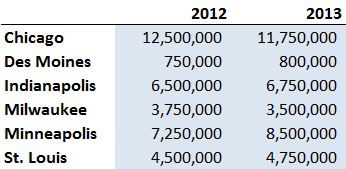
Download the attached worksheet containing sample sales data by city:
In Excel 1997-2003
Click “Insert | Chart.” In the wizard that pops up, do the following:
1. Chart Type. Choose “Column” and select the first subtype.
2. Chart Source Data. Enter the following:
a. For data range, choose B4:C9 (shown in light blue).
b. Select “Columns” for the series.
c. On the “Series” tab, select cells A4:A9 for the category labels.
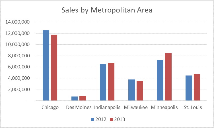
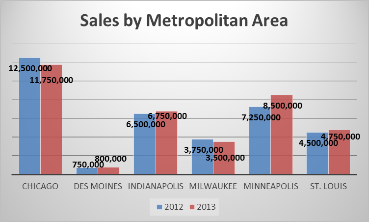
3. Chart Options. Add “Sales by Metropolitan Area” for the title and add a legend.
4. Chart Location. Choose “As object in” and select “Sheet1.”
In Excel 2007-2013
1. Drag your mouse to highlight cells B4:C9 (shown in light blue).
2. On the “Insert” tab, click “Insert Column Chart.”
3. Choose “2-D Clustered Column.”
4. On the new “Chart Tools | Design” tab on the ribbon, choose “Select Data.” In the dialog box:
a. Change the horizontal (category) labels to A4:A9 and click “OK.”
b. Edit Series1 and choose B3 for the series name.
c. Edit Series2 and choose C3 for the series name.
5. On the new chart, depending on which version of Excel you are using, either double-click the words “Chart Title” or click on the “Chart Tools | Layout” tab and add the title “Sales by Metropolitan Area.”
Next Steps
Invest some time in the worksheet exploring the chart options. Go through the chart tools tabs and experiment with the tools. Most are self-explanatory or will present you with a preview before you select the final options.
After all, what better way is there to learn than by doing it?
PRYOR+ 7-DAYS OF FREE TRAINING
Courses in Customer Service, Excel, HR, Leadership,
OSHA and more. No credit card. No commitment. Individuals and teams.
When you’re manually writing a function-based formula in a cell, you’re prone to make syntax errors. Also, it requires you to remember the syntax for each function. The Microsoft Excel Function Wizard, on the other hand, provides the user with a list of predefined formulas and makes them easy to implement. It is perfect for quickly creating valid functions.
The function wizard is handy when you can’t remember which function to use, or how to use it. In this article, we’ll show you how to use Insert Function Wizard in Excel.
How to create a formula in Excel by using the Insert Function Wizard
An Excel function is a predefined formula or an expression that performs specific calculations in a cell or a range of cells.
Function Wizard allows you to access all Excel’s pre-defined data analysis functions.
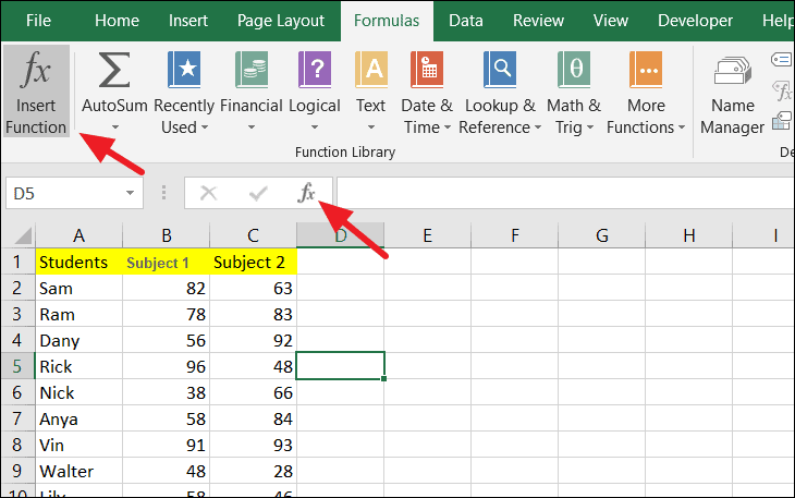
First, select the cell where you the output (answer) to appear.
Then to open the function wizard, go to the Formulas tab and click the ‘Insert Function’ option on the Function Library group. Or, you can click the Insert Function button ‘fx’ to the left of the formula bar.
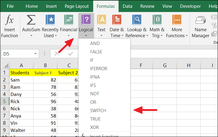
You can also choose a function from any one of the categories available in the ‘Function Library’ under the Formulas tab.
Alternatively, type an equal sign (=) in the cell where you want the output and select a function from the drop-down (from the Name box) to the left of the formula bar.
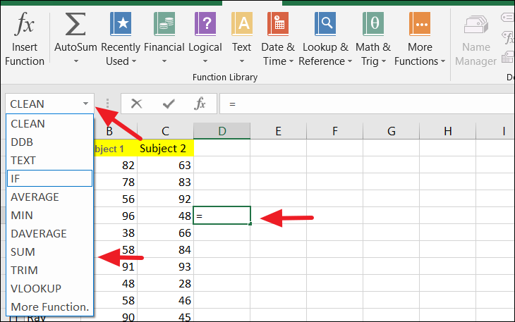
This drop-down menu will display 10 most recently used functions by you.
Inserting an Excel Function
The structure of a function always starts with an equal sign (=), followed by the function name, and the parameters of the function enclosed in parentheses.
When the Insert function wizard opens up, you can insert a function in three different ways.
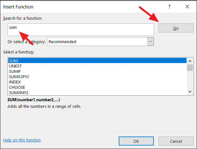
If you already know the function name, enter it in the ‘Search for a function’ field and click the ‘Go’ button.
If you forgot the function or not sure exactly what function you need to use, type a brief description of what you want to do in the ‘Search for a function’ field and click ‘Go’. For example, you can type something like this: ‘remove space’ for removing extra spaces in the text string, or ‘current date and time’ for returning the current date and time.
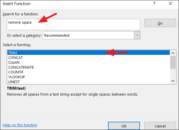
Although you won’t find an exact match for the description, you would at least get a list of closely related functions in the ‘Select a function’ box. If you click on a function, you can read a short description of that function right under the ‘Select a function’ box.
If you know what category the function belongs to, click on the drop-down menu next to ‘Select a category’ and pick one of the 13 categories listed there. All the functions under the selected category will be listed in the ‘Select a function’ box.
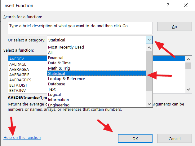
If you want to know more about the selected function, click the ‘Help on this function’ link at the bottom left corner of the dialog box. This will take you to the Microsoft ‘Support’ page where you can learn the description of the formula syntax and usage of the function.
Once you’ve found the right function for your task, select it and click ‘OK’.
Specify the Arguments
Function arguments are the values that functions need to perform calculations, they can be numbers, text strings, logical values, arrays, error values, or cell references. They can also use constants, formulas, or other functions as arguments.
For example, we’ll see how to insert SUM (one of the most frequently used functions in Excel) in the formula to add all the values in a range of cells.
Once you selected a function in the function ‘Insert Function’ wizard and clicked ‘OK’, it will take you to another wizard called ‘Function Arguments’.
There, you need to enter the function’s arguments. To enter an argument, just type a cell reference or a range, or constants directly into the argument box. You can insert as many arguments as you want by clicking on the next box.
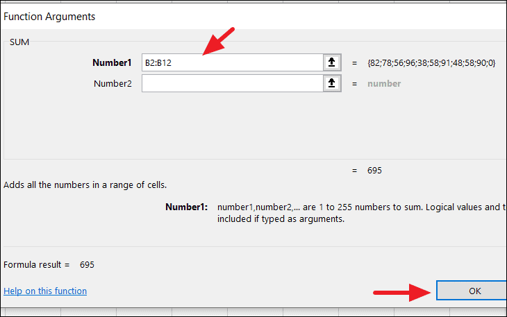
Alternatively, click in the argument’s box, and then select a cell or a range of cells in the spreadsheet using the mouse. Then, click ‘OK’.
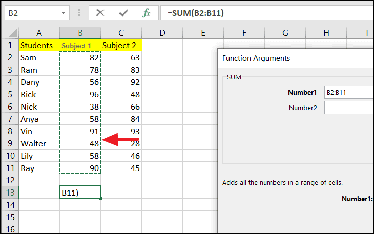
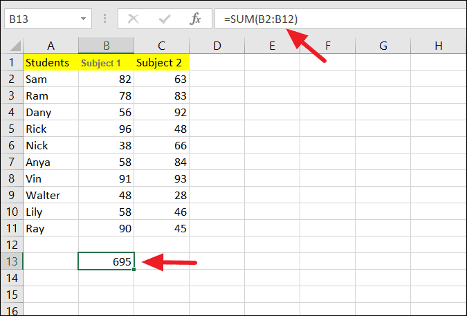
After you have specified all the arguments, click the ‘OK’ button. The answer will be displayed in the selected cell and the completed formula will be displayed in the Formula bar.
In our earlier article, we discussed how we can do quick data analysis using Pivot Table functionality in Excel. In this article, we will discuss how we can consolidate data across multiple sheets and prepare quick reports with the help of Pivot Tables.
Let us quickly understand with the help of an example.
We have multiple data sheets showing revenues by regions. Each sheet has name of products on rows and months listed in the columns. We are asked to prepare a summary showing performance by countries.
Before starting to consolidate the data, we have to ensure that
- Each sheet has the same structure. Meaning, that apart from the data the number of rows, columns, column headers should be the same.
- There are no blank rows or columns in between
- There are no totals, subtotals in between.
- Each column has a header.
Once we ensure that all the above criteria are met, we can start consolidating the data.
If we have limited number of sheets, we can add up all the data to create a summary, but this is not the most efficient method. It requires lot of manual intervention and there are also chances of errors. Also, we cannot easily change the output once the consolidation is done as it would require lot of manual intervention.
Excel has an inbuilt feature which can be used to consolidate data in multiple sheets efficiently. It is the Pivot Table Wizard. To activate the Pivot Table Wizard, Press Alt & D. Pressing Alt & D activates the Office Access Key. Then Press P. This activates the Pivot Table Wizard.
With Pivot table wizard, we can create a data summary with Just 3 steps.
Step 1
First, it asks if we want to consolidate data using Microsoft Excel list or database, External data source or Multiple consolidation ranges.
We will select Multiple consolidation ranges, as all the data is present in multiple sheets in a single file.
Then it asks if we want to create a Pivot Table or a PivotChart Report.
We will select Create a Pivot Table.
Then Click on Next.
Step 2a
In the second step, it asks if we want to create a Pivot Table report that uses ranges from one or more sheets. Also, how many page fields are required.
Here we will choose the option, I will create the Page Fields.
Then Click Next.
Step 2b
This is the most important step.
Here we have to select the data range.
Click on range and then select the data range from the first sheet.
Then Click Add.
Repeat this step for all the sheets which has the data to be consolidated.
Once we select all the data ranges. It asks, how many page fields do we want? We will select the option 1.
Then, Select the ranges (one by one) in the Range section, and then give a name to them in Field one (as shown in the above screen shot).
One we give a name to all the data ranges, Click Next.
Step 3
In the third step it asks, where we want to put the pivot table report. Whether in a new worksheet or the existing worksheet?
We will select the first option (New worksheet) and then Press Finish. We get the Pivot table report in a new sheet.
We get a consolidated data Pivot table in a new sheet.
This pivot table has all the features which were covered in our previous article. Some of them are as follows.
- We can change the report layout by changing the selection of the Pivot table fields.
- We can change the number format
- Sort the products by totals
- Calculate the percent of total sales, or average sales based on the requirement
- Change the Pivot table design
- Remove grand totals and Pivot table headers.
- Use the Pivot table slicer to create dynamic outputs.
There are multiple other options available which can be explored for further refinements as needed.
This is how we can consolidate data in multiple sheets with just a few clicks for data analysis or preparing dynamic reports. In case you have any questions, please post in the comment section. Enjoy learning.
Skip to content
The Pivot Table Wizard isn’t available on the Ribbon in Excel 2007. To open the Pivot Table Wizard, you can use the keyboard shortcut — Alt + D, P — as described in the article on creating a pivot table from multiple sheets.
Another option is to add the Pivot Table Wizard button to your Quick Access Toolbar (QAT), by following the steps below.
Customize the QAT
To add the Pivot Table Wizard to your QAT, follow these steps:
- Click on the Customize Quick Access Toolbar button
- Click More Commands

- From the ‘Choose commands from’ drop down list, select ‘Commands Not in the Ribbon’

- In the list of commands, click PivotTable and PivotChart Wizard
- Click the Add button, then click OK

Open the Pivot Table Wizard
Now that the Pivot Table Wizard button has been added to the QAT, you can click it to open the Pivot Table Wizard.

___________
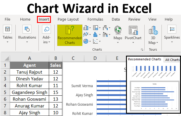
Chart Wizard in Excel (Table of Content)
- Chart Wizard in Excel
- How to Use a Chart Wizard in Excel?
Chart Wizard in Excel
Chart Wizard in Excel is used to apply different charts, which can be Column, Bar, Pie, Area, Line, etc. Chart Wizard, which is now named as Chart in the new version of MS Office, is available in the insert menu tab. To create a chart in Excel, select data with at least one parameter that can be mapped, then from the Insert menu tab, select any chart type of choice. This will easily create generate the chart. We can even change the colour of the chart, add data labels, a trend to make it more meaningful.
How to Use a Chart Wizard in Excel?
Let’s understand the working of it with the below simple steps.
You can download this Chart Wizard Excel Template here – Chart Wizard Excel Template
Example #1 – Create a Chart using Wizard
You can use any data to convert it into the chart by using this wizard. Let’s consider the below data table as shown in the below table and create a chart using Chart wizard.
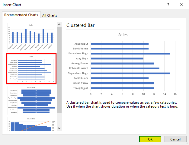
- First, select the data from which you want to create the chart, then go to the Insert tab and select Recommended Charts Tab.
- Select the chart and then click on OK.
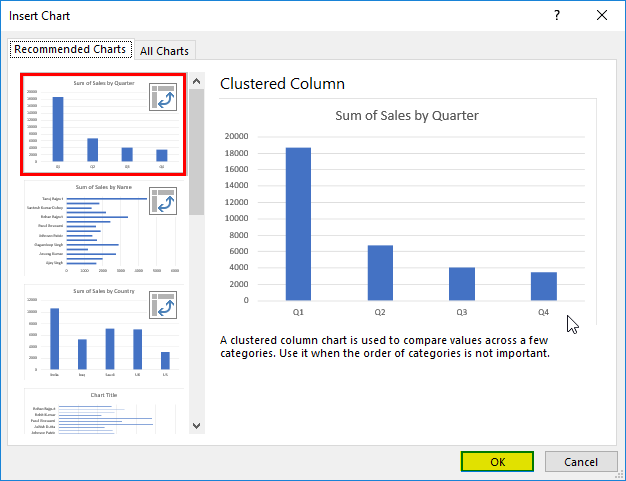
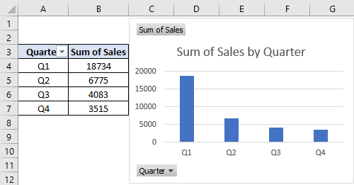
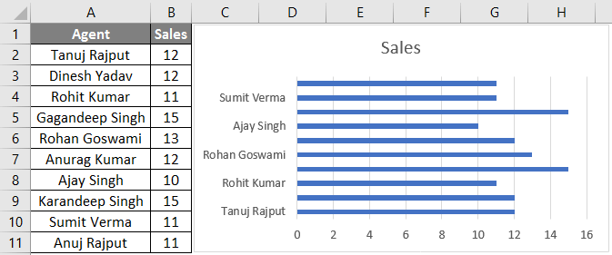
- And the output will be as shown in the below figure:
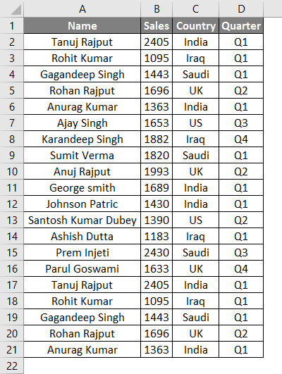
Example #2 – Create a Chart for Sales Data
Let’s consider the below data set as shown in the below table.
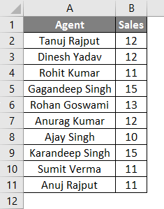
- Select the sales data from which you want to create the chart, then go to the Insert tab and select Recommended Charts Tab.
- Select the chart and then click on OK.
- And the output will be as shown in the below figure:
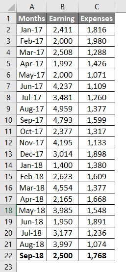
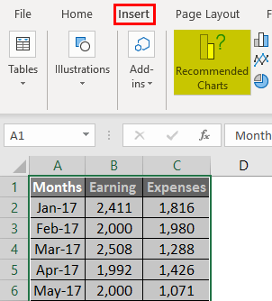
Example #3 – Create a Chart for Earning and Expenses Data
Let’s consider the below earning and expenses data set to create the chart using chart wizard.
Here are the steps as follows:
- First, select the data, then go to the Insert tab and select Recommended Chart Tab.
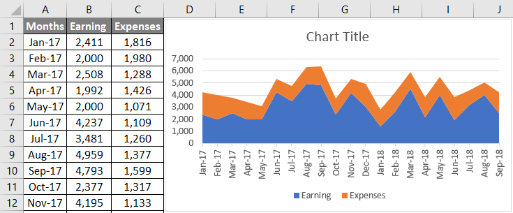
- Pick any chart type, and then just click OK.
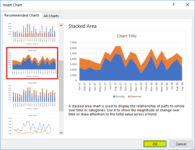
- And the output will be as shown in the below figure:
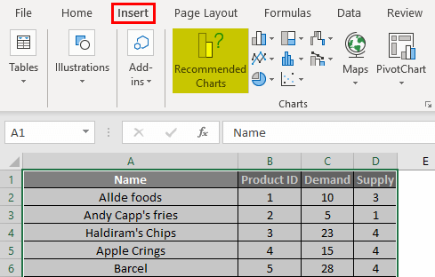
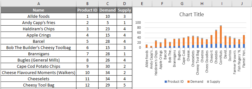
Example #4 – Create a Chart for Demand and supply Data
Let’s consider the below demand and supply data to create a chart using chart wizard in excel.

The steps are the same as we used in the previous examples; just select the below data, then Go to the insert tab and select Recommended Chart Tab.
Select the chart which you want to create, then click OK.

And the output will be as shown in the below figure:
Things to Remember
- The Chart Wizard is very simple and easy, and it is used to create an attractive chart by using simple mouse clicks.
- The Chart wizard provides simple steps to create complex charts.
Recommended Articles
This has been a guide to Chart Wizard. Here we discussed How to use a Chart Wizard in Excel along with examples and a downloadable excel template. You may also look at these useful excel articles –
- Excel Stacked Bar Chart
- Excel Flowchart
- Marimekko Chart Excel
- Histogram Chart Excel