
How to avoid broken formulas
Excel for Microsoft 365 Excel for Microsoft 365 for Mac Excel for the web Excel 2021 Excel 2021 for Mac Excel 2019 Excel 2019 for Mac Excel 2016 Excel 2016 for Mac Excel 2013 Excel for iPad Excel for Android tablets Excel 2010 Excel 2007 Excel Starter 2010 More…Less
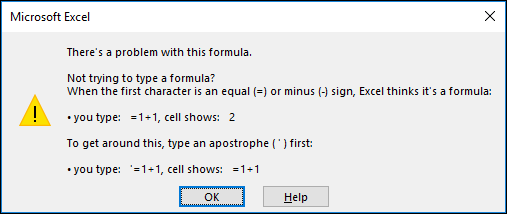
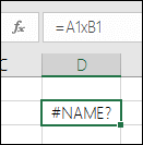
If Excel can’t resolve a formula you’re trying to create, you may get an error message like this one:
Unfortunately, this means that Excel can’t understand what you’re trying to do, so you’ll need to update your formula or make sure you’re using the function correctly.
Tip: There are a few common functions where you might run into issues, check out COUNTIF, SUMIF, VLOOKUP, or IF to learn more. You can also see a list of functions here.
Return to the cell with the broken formula, which will be in edit mode, and Excel will highlight the spot where it’s having a problem. If you still don’t know what to do from there and want to start over, you can press ESC again, or select the Cancel button in the formula bar, which will take you out of edit mode.

If you want to move forward, then the following checklist provides troubleshooting steps to help you figure out what may have gone wrong. Select the headings to learn more.
Note: If you’re using Microsoft 365 for the web, you may not see the same errors, or the solutions may not apply.
Excel throws a variety of pound (#) errors such as #VALUE!, #REF!, #NUM, #N/A, #DIV/0!, #NAME?, and #NULL!, to indicate something in your formula isn’t working properly. For example, the #VALUE! error is caused by incorrect formatting or unsupported data types in arguments. Or, you’ll see the #REF! error if a formula refers to cells that have been deleted or replaced with other data. Troubleshooting guidance will differ for each error.
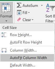
Note: #### is not a formula-related error. It just means that the column isn’t wide enough to display the cell contents. Simply drag the column to widen it, or go to Home > Format > AutoFit Column Width.
Refer to any of the following topics corresponding to the pound error you see:
-
Correct a #NUM! error
-
Correct a #VALUE! error
-
Correct a #N/A error
-
Correct a #DIV/0! error
-
Correct a #REF! error
-
Correct a #NAME? error
-
Correct a #NULL! error
Each time you open a spreadsheet that contains formulas referring to values in other spreadsheets, you’ll be prompted to update the references or leave them as-is.
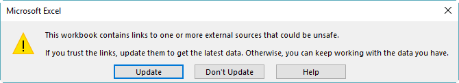
Excel displays the above dialog box to make sure that the formulas in the current spreadsheet always point to the most updated value in case the reference value has changed. You can choose to update the references, or skip if you don’t want to update. Even if you choose to not update the references, you can always manually update the links in the spreadsheet whenever you want.
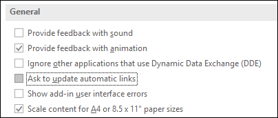
You can always disable the dialog box from appearing at start up. To do that, go to File > Options > Advanced > General, and clear the Ask to update automatic links box.
Important: If this is the first time you’re working with broken links in formulas, if you need a refresher on resolving broken links, or if you don’t know whether to update the references, see Control when external references (links) are updated.
If the formula doesn’t display the value, follow these steps:
-
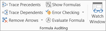
Make sure Excel is set to show formulas in your spreadsheet. To do this, select the Formulas tab, and in the Formula Auditing group, select Show Formulas.
Tip: You can also use the keyboard shortcut Ctrl + ` (the key above the Tab key). When you do this, your columns will automatically widen to display your formulas, but don’t worry, when you toggle back to the normal view, your columns will resize.
-
If the step above still doesn’t resolve the issue, it’s possible the cell is formatted as text. You can right-click on the cell and select Format Cells > General (or Ctrl + 1), then press F2 > Enter to change the format.
-
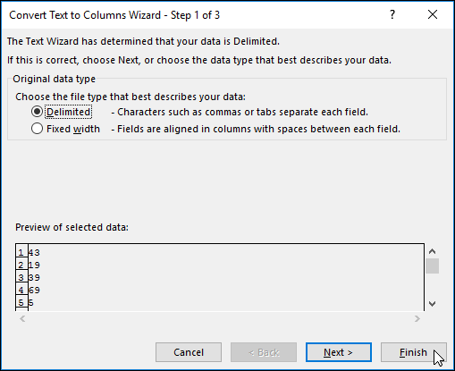
If you have a column with a large range of cells that are formatted as text, you can select the range, apply the number format of your choice, and go to Data > Text to Column > Finish. This will apply the format to all of the selected cells.

When a formula does not calculate, you’ll need to check if automatic calculation is enabled in Excel. Formulas won’t calculate if manual calculation is enabled. Follow these steps to check for Automatic calculation.
-
Select the File tab, select Options, and then select the Formulas category.
-
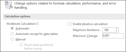
In the Calculation options section, under Workbook Calculation, make sure the Automatic option is selected.
For more information on calculations, see Change formula recalculation, iteration, or precision.
A circular reference occurs when a formula refers to the cell that it’s located in. The fix is to either move the formula to another cell, or change the formula syntax to one that avoids circular references. However, in some scenarios you may need circular references because they cause your functions to iterate—repeat until a specific numeric condition is met. In such cases, you’ll need to enable Remove or allow a circular reference.
For more information on circular references, see Remove or allow a circular reference.
If your entry doesn’t start with an equal sign, it isn’t a formula, and won’t be calculated—a common mistake.
When you type something like SUM(A1:A10), Excel shows the text string SUM(A1:A10) instead of a formula result. Alternatively, if you type 11/2, Excel shows a date, such as 2-Nov or 11/02/2009, instead of dividing 11 by 2.
To avoid these unexpected results, always start the function with an equal sign. For example, type: =SUM(A1:A10) and =11/2.
When you use a function in a formula, each opening parenthesis needs a closing parenthesis for the function to work correctly. Make sure that all parentheses are part of a matching pair. For example, the formula =IF(B5<0),»Not valid»,B5*1.05) won’t work because there are two closing parentheses, but only one opening parenthesis. The correct formula would look like this: =IF(B5<0,»Not valid»,B5*1.05).
Excel functions have arguments—values you need to provide for the function to work. Only a few functions (such as PI or TODAY) take no arguments. Check the formula syntax that appears as you start typing in the function, to make sure the function has the required arguments.
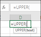
For example, the UPPER function accepts only one string of text or cell reference as its argument: =UPPER(«hello») or =UPPER(C2)
Note: You’ll see the function’s arguments listed in a floating function reference toolbar beneath the formula as you’re typing it.
Also, some functions, such as SUM, require numerical arguments only, while other functions, such as REPLACE, require a text value for at least one of their arguments. If you use the wrong data type, functions might return unexpected results or show a #VALUE! error.
If you need to quickly look up the syntax of a particular function, see the list of Excel functions (by category).
Don’t enter numbers formatted with dollar signs ($) or decimal separators (,) in formulas because dollar signs indicate Absolute References and commas are argument separators. Instead of entering $1,000, enter 1000 in the formula.
If you use formatted numbers in arguments, you’ll get unexpected calculation results, but you may also see the #NUM! error. For example, if you enter the formula =ABS(-2,134) to find the absolute value of -2134, Excel shows the #NUM! error, because the ABS function accepts only one argument, and it sees the -2, and 134 as separate arguments.
Note: You can format the formula result with decimal separators and currency symbols after you enter the formula using unformatted numbers (constants). It’s generally not a good idea to put constants in formulas, because they can be hard to find if you need to update later and they’re more prone to being typed incorrectly. It’s much better to put your constants in cells, where they’re out in the open and easily referenced.
Your formula might not return expected results if the cell’s data type can’t be used in calculations. For example, if you enter a simple formula =2+3 in a cell that’s formatted as text, Excel can’t calculate the data you entered. All you’ll see in the cell is =2+3. To fix this, change the cell’s data type from Text to General like this:
-
Select the cell.
-
Select Home and select the arrow to expand the Number or Number Format group (or press Ctrl + 1). Then select General.
-
Press F2 to put the cell in the edit mode, and then press Enter to accept the formula.
A date you enter in a cell that’s using the Number data type might be shown as a numeric date value instead of a date. To show a number as a date, pick a Date format in the Number Format gallery.
It’s fairly common to use x as the multiplication operator in a formula, but Excel can only accept the asterisk (*) for multiplication. If you use constants in your formula, Excel shows an error message and can fix the formula for you by replacing the x with the asterisk (*).
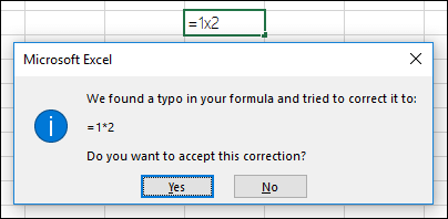
However, if you use cell references, Excel will return a #NAME? error.
If you create a formula that includes text, enclose the text in quotation marks.
For example, the formula =»Today is » & TEXT(TODAY(),»dddd, mmmm dd») combines the text «Today is » with the results of the TEXT and TODAY functions, and returns say something like Today is Monday, May 30.
In the formula, «Today is » has a space before the ending quotation mark to provide the blank space you want between the words «Today is» and «Monday, May 30.» Without quotation marks around the text, the formula might show the #NAME? error.
You can combine (or nest) up to 64 levels of functions within a formula.
For example, the formula =IF(SQRT(PI())<2,»Less than two!»,»More than two!») has 3 levels of functions; the PI function is nested inside the SQRT function, which in turn is nested inside the IF function.
When you type a reference to values or cells in another worksheet, and the name of that sheet has a non-alphabetical character (such as a space), enclose the name in single quotation marks (‘).
For example, to return the value from cell D3 in a worksheet named Quarterly Data in your workbook, type: =’Quarterly Data’!D3. Without the quotation marks around the sheet name, the formula shows the #NAME? error.
You can also select the values or cells in another sheet to refer to them in your formula. Excel then automatically adds the quotation marks around the sheet names.
When you type a reference to values or cells in another workbook, include the workbook name enclosed in square brackets ([]) followed by the name of the worksheet that has the values or cells.
For example, to refer to cells A1 through A8 on the Sales sheet in the Q2 Operations workbook that’s open in Excel, type: =[Q2 Operations.xlsx]Sales!A1:A8. Without the square brackets, the formula shows the #REF! error.
If the workbook isn’t open in Excel, type the full path to the file.
For example, =ROWS(‘C:My Documents[Q2 Operations.xlsx]Sales’!A1:A8).
Note: If the full path has space characters, enclose the path in single quotation marks (at the beginning of the path and after the name of the worksheet, before the exclamation point).
Tip: The easiest way to get the path to the other workbook is to open the other workbook, then from your original workbook, type =, and use Alt+Tab to shift to the other workbook. Select any cell on the sheet you want, then close the source workbook. Your formula will automatically update to display the full file path and sheet name along with the required syntax. You can even copy and paste the path and use wherever you need it.
Dividing a cell by another cell that has zero (0) or no value results in a #DIV/0! error.
To avoid this error, you can address it directly and test for the existence of the denominator. You could use:
=IF(B1,A1/B1,0)
Which says IF(B1 exists, then divide A1 by B1, otherwise return a 0).
Always check to see if you have any formulas that refer to data in cells, ranges, defined names, worksheets, or workbooks before you delete anything. You can then replace these formulas with their results before you remove the referenced data.
If you can’t replace the formulas with their results, review this information about the errors and possible solutions:
-
If a formula refers to cells that have been deleted or replaced with other data, and if it returns a #REF! error, select the cell with the #REF! error. In the formula bar, select #REF! and delete it. Then enter the range for the formula again.
-
If a defined name is missing, and a formula that refers to that name returns a #NAME? error, define a new name that refers to the range you want, or change the formula to refer directly to the range of cells (for example, A2:D8).
-
If a worksheet is missing, and a formula that refers to it returns a #REF! error, there’s no way to fix this, unfortunately—a worksheet that’s been deleted can’t be recovered.
-
If a workbook is missing, a formula that refers to it remains intact until you update the formula.
For example, if your formula is =[Book1.xlsx]Sheet1′!A1 and you no longer have Book1.xlsx, the values referenced in that workbook stay available. However, if you edit and save a formula that refers to that workbook, Excel shows the Update Values dialog box and prompts you to enter a file name. Select Cancel, and then make sure this data isn’t lost by replacing the formulas that refer to the missing workbook with the formula results.
Sometimes, when you copy the contents of a cell, you want to paste just the value and not the underlying formula that’s displayed in the formula bar.
For example, you might want to copy the resulting value of a formula to a cell on another worksheet. Or you might want to delete the values that you used in a formula after you copied the resulting value to another cell on the worksheet. Both of these actions cause an invalid cell reference error (#REF!) to appear in the destination cell, because the cells that contain the values you used in the formula can no longer be referenced.
You can avoid this error by pasting the resulting values of formulas, without the formula, in destination cells.
-
On a worksheet, select the cells that contain the resulting values of a formula that you want to copy.
-
On the Home tab, in the Clipboard group, select Copy
.
Keyboard shortcut: Press CTRL+C.
-
Select the upper-left cell of the paste area.
Tip: To move or copy a selection to a different worksheet or workbook, select another worksheet tab or switch to another workbook, and then select the upper-left cell of the paste area.
-
On the Home tab, in the Clipboard group, select Paste
, and then select Paste Values, or press Alt > E > S > V > Enter for Windows, or Option > Command > V > V > Enter on a Mac.
 .
.
 , and then select Paste Values, or press Alt > E > S > V > Enter for Windows, or Option > Command > V > V > Enter on a Mac.
To understand how a complex or nested formula calculates the final result, you can evaluate that formula.
-
Select the formula you want to evaluate.
-
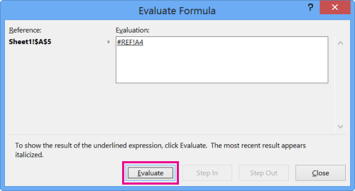
Select Formulas > Evaluate Formula.
-
Select Evaluate to examine the value of the underlined reference. The result of the evaluation is shown in italics.
-
If the underlined part of the formula is a reference to another formula, select Step In to show the other formula in the Evaluation box. Select Step Out to go back to the previous cell and formula.
The Step In button isn’t available the second time the reference appears in the formula—or if the formula refers to a cell in another workbook.
-
Continue until each part of the formula has been evaluated.
The Evaluate Formula tool won’t necessarily tell you why your formula is broken, but it can help point out where. This can be a very handy tool in larger formulas where it might otherwise be difficult to find the problem.
Notes:
-
Some parts of the IF and CHOOSE functions won’t be evaluated, and the #N/A error might appear in the Evaluation box.
-
Blank references are shown as zero values (0) in the Evaluation box.
-
Some functions are recalculated every time the worksheet changes. Those functions, including the RAND, AREAS, INDEX, OFFSET, CELL, INDIRECT, ROWS, COLUMNS, NOW, TODAY, and RANDBETWEEN functions, can cause the Evaluate Formula dialog box to show results that are different from the actual results in the cell on the worksheet.
-

Need more help?
You can always ask an expert in the Excel Tech Community or get support in the Answers community.
Tip: If you’re a small business owner looking for more information on how to get Microsoft 365 set up, visit Small business help & learning.
See Also
Overview of formulas in Excel
Excel help & learning
Need more help?
6 Main Reasons for Excel Formula Not Working (with Solution)
- Reason #1 – Cells Formatted as Text
- Reason #2 – Accidentally Typed the keys CTRL + `
- Reason #3 – Values are Different & Result is Different
- Reason #4 – Don’t Enclose Numbers in Double Quotes
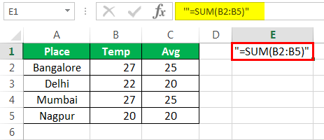
- Reason #5 – Check If Formulas are Enclosed in Double Quotes
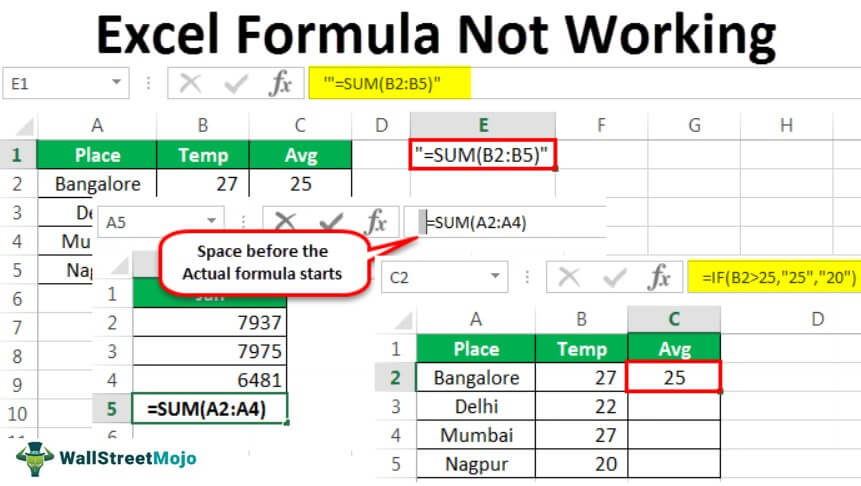
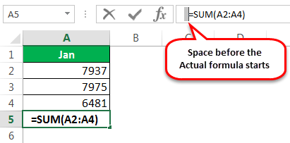
- Reason #6 – Space Before the Excel Formula
Table of contents
- 6 Main Reasons for Excel Formula Not Working (with Solution)
- #1 Cells Formatted as Text
- Solution
- #2 Accidentally Typed the keys CTRL + `
- Solution
- #3 Values are Different & Result is Different
- Solution
- #4 Don’t Enclose Numbers in Double Quotes
- #5 Check If Formulas are Enclosed in Double Quotes
- #6 Space Before the Excel Formula
- Recommended Articles
- #1 Cells Formatted as Text
You are free to use this image on your website, templates, etc, Please provide us with an attribution linkArticle Link to be Hyperlinked
For eg:
Source: Excel Formula Not Working (wallstreetmojo.com)
#1 Cells Formatted as Text
Now let us look at the solutions for the reasons given above for the Excel formula not working.
Now take a look at the first possibility of the formula showing the formula itself, not the result of the formula. For example, look at the below image where the SUM function in excelThe SUM function in excel adds the numerical values in a range of cells. Being categorized under the Math and Trigonometry function, it is entered by typing “=SUM” followed by the values to be summed. The values supplied to the function can be numbers, cell references or ranges.read more shows the formula, not the result.
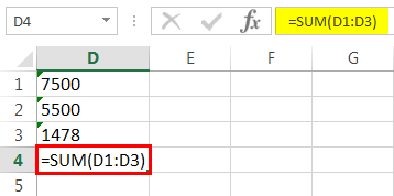
The first thing we need to look into is the format of the cells; these cells are D1, D2, and D3. So, now take a look at the format of these cells.
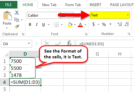
It is formatted as text. When the cells are formatted as text, Excel cannot read numbers and return the result for your applied formula.
Solution
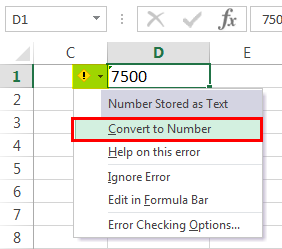
Change the format of the cells to “General” or “Convert to Number.”
- We must first select the cells. Then, on the left-hand side, we can see one small icon. Click on that icon, and choose the option “Convert to Number.”

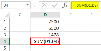
- Now, we must see the result of the formula.

- We are still not getting the result we are looking for. Now, we need to examine whether the formula cell is formatted as text or not.

- Yes, it is formatted as text, so change the cell format to “GENERAL” or “NUMBER.” We must see the result now.


#2 Accidentally Typed the keys CTRL + `
Often in Excel, when working in a hurry, we tend to type keys that are not required, which is an accidental incident. But if we do not know which key we typed, we may get an unusual result.
One such moment is SHOW FORMULAS in excelIn Excel, we can display formulas to investigate the procedure’s relationship. To begin, select the formula tab, then formula auditing, and finally show formulas. In addition, there is a keyboard shortcut for it.read more shortcut key CTRL + `. If we have accidentally typed this key, we may see the result like the picture below.
As we said, the reason could be the accidental pressing of the show formula shortcut key.
Solution
The solution is to try typing the same key again to get back the results of the formula rather than the formula itself.
#3 Values are Different & Result is Different
Sometimes, we see different numbers in Excel, but the formula shows different results. For example, the below image displays one such situation.
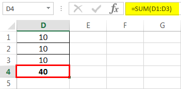
In cells D1, D2, and D3, we have 10 as the value. In cell D4, we have applied the SUM function to get the total value of cells D1, D2, and D3. But the result says 40 instead of 30.
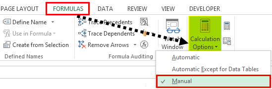
All the Excel file calculations are set to automatic. But to enhance the speed of the large data files, the user might have changed the auto calculation to a manual one.
Solution
We can fix this in two ways. One is we can turn on the calculation to “Automatic.”
Either we can do one more thing. We can also press the shortcut key F9, which is nothing but “Calculate Now” under the “Formulas” bar.
#4 Don’t Enclose Numbers in Double Quotes
We must pass the numerical values to get the desired result in situations inside the formula. For example, please take a look at the below image; it shows cities and the average temperature in the city.
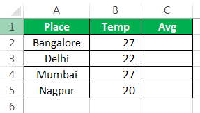
If the temperature is greater than 25, then the average should be 25, and if the temperature is less than 25, then the average should be 20. Finally, we will apply the IF condition in excelIF function in Excel evaluates whether a given condition is met and returns a value depending on whether the result is “true” or “false”. It is a conditional function of Excel, which returns the result based on the fulfillment or non-fulfillment of the given criteria.
read more to get the results.

We have supplied the numerical results double-quotes =IF (B2>25,” 25″,” 20″). Unfortunately, when the numbers are passed in double-quotes, Excel treats them as text values. Therefore, we cannot do any calculations with text numbers.
Always pass the numerical values without double quotes like the below image.
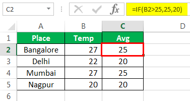
Now, we can do all sorts of calculations with these numerical values.
#5 Check If Formulas are Enclosed in Double Quotes
We need to ensure formulas are not wrapped in double quotes. It happens when we copy formulas from online websites and paste them as it is. If the formula is mentioned in double quotes for understanding, we need to remove double quotes and paste them. Otherwise, we may get only the formulas, not the result of the formula.
#6 Space Before the Excel Formula
We all humans make mistakes. Typing mistake is one of the errors for the Excel formula not working. We usually commit day in and day out in our workplace. If we type one or more spaces before we start our formula, it breaks the rule of the formulas in Excel. As a result, we may end up with only the Excel formula, not the result of the formula.
Recommended Articles
This article has been a guide to Excel Formula Not Working and Updating. Here, we discuss the Top 6 reasons and solutions for those Excel formulas not working and updating, practical examples, and a downloadable Excel template. You may learn more about Excel from the following articles: –
- Excel Minus Formula
- Excel VBA IFERROR
- Formula Excel Errors
- Max Formula in Excel
If you work with formulas in Excel, sooner or later you will encounter the problem where Excel formulas don’t work at all (or give the wrong result).
While it would have been great had there been only a few possible reasons for malfunctioning formulas. Unfortunately, there are too many things that can go wrong (and often does).
But since we live in a world that follows the Pareto principle, if you check for some common issues, it’s likely to solve 80% (or maybe even 90% or 95% of the issues where formulas are not working in Excel).
And in this article, I will highlight those common issues that are likely the cause of your Excel formulas not working.
So let’s get started!
Incorrect Syntax of the Function
Let me start by pointing out the obvious.
Every function in Excel has a specific syntax – such as the number of arguments it can take or the type of arguments it can accept.
And in many cases, the reason your Excel formulas are not working or gives the wrong result could be an incorrect argument (or missing arguments).
For example, the VLOOKUP function takes three mandatory arguments and one optional argument.
If you provide a wrong argument or don’t specify the optional argument (where it’s needed for the formula to work), it’s going to give you a wrong result.
For example, suppose you have a dataset as shown below where you need to know the score of Mark in Exam 2 (in cell F2).

If I use the below formula, I will get the wrong result, because I am using the wrong value in the third argument (one that asks for Column Index number).
=VLOOKUP(A2,A2:C6,2,FALSE)

In this case, the formula calculates (as it returns a value), but the result is incorrect (instead of score in Exam 2, it gives the score in Exam 1).
Another example where you need to be cautious about the arguments is when using VLOOKUP with the approximate match.
Since you need to use an optional argument to specify where you want VLOOKUP to do an exact match or an approximate match, not specifying this (or using the wrong argument) can cause issues.
Below is an example where I have the marks data for some students and I want to extract marks in Exam 1 for the students in the table on the right.

When I use the below VLOOKUP formula it gives me an error for some names.
=VLOOKUP(E2,$A$2:$C$6,2)

This happens as I have not specified the last argument (which is used to determine whether to do an exact match or approximate match). When you don’t specify the last argument, it automatically does an approximate match by default.
Since we needed to do an exact match in this case, the formula returns an error for some names.
While I have taken the example of the VLOOKUP function, in this case, this is something that can be applicable for many Excel formulas that have optional arguments as well.
Also read: Identify Errors Using Excel Formula Debugging
Extra Spaces Causing Unexpected Results
Leading, trailing spaces are hard to find out and can cause issues when you use a cell that has these in formulas.
For example, in the below example, if I try to use VLOOKUP to fetch the score for Mark, it gives me the #N/A error (the not available error).

While I can see that the formula is correct and the name ‘Mark’ is clearly there is the list, what I can not see is that there is a trailing space in the cell that has the name (in cell D2).

Excel doesn’t consider the content of these two cells the same and therefore it considers it a mismatch when fetching the value using VLOOKUP (or it could be any other lookup formula).
To fix this issue, you need to remove these extra space characters.
You can do this by using any of the following methods:
- Clean the cell and remove any leading/trailing spaces before using it in formulas
- Use the TRIM function within the formula to make sure any leading/trailing/double spaces are ignored.
In the above example, you can use the below formula instead to make sure it works.
=VLOOKUP(TRIM(D2),$A$2:$B$6,2,0)
While I have taken the VLOOKUP example, this is also a common issue when working with TEXT functions.
For example, if I use the LEN function to count the total number of characters in a cell, if there are leading or trailing spaces, these would also be counted and give the wrong result.
Take away / How to Fix: If possible, clean your data by removing any leading/trailing or double spaces before using these in formulas. If you can not change the original data, use the TRIM function in formulas to take care of this.
Using Manual Calculation Instead of Automatic
This one setting can drive you crazy (if you don’t know it’s what’s causing all the issues).
Excel has two calculation modes – Automatic and Manual.
By default, the automatic mode is enabled, which means that in case I use a formula or make any changes in the existing formulas, it automatically (and instantly) makes the calculation and gives me the result.
This is the setting we are all used to.
In the automatic setting, whenever you make any change in the worksheet (such as entering a new formula to even some text in a cell), Excel automatically recalculates everything (yes, everything).
But in some cases, people enable the manual calculation setting.
This is mostly done when you have a heavy Excel file with a lot of data and formulas. In such cases, you may not want Excel to recalculate everything when you make small changes (as it may take a few seconds or even minutes) for this recalculation to complete.
If you enable manual calculation, Excel will not calculate unless you force it to.
And this may make you think that your formula is not calculating.
All you need to do in this case is either set the calculation back to automatic or force a recalculation by hitting the F9 key.
Below are the steps to change the calculation from manual to automatic:
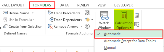
- Click the Formula tab

- Click on Calculation Options
- Select Automatic


Important: In case you’re changing the calculation from manual to automatic, it’s a good idea to create a backup of your workbook (just in case this makes your workbook hang or makes Excel crash)
Take away / How to Fix: If you notice that your formulas are not giving the expected result, try something simple in any cell (such as adding 1 to an existing formula. Once you identify the issue as the one where calculation mode needs to be changed, do a force calculation by using F9.
Deleting Rows/Column/Cells Leading to #REF! Error
One of the things that can have a devastating effect on your existing formulas in Excel is when you delete any row/column which has been used in calculations.
When this happens, sometimes, Excel adjusts the reference itself and makes sure that the formulas are working fine.
And sometimes… it can not.
Thankfully, one clear indication that you get when formulas break on deleting cells/rows/columns is the #REF! error in the cells. This is a reference error that tells you that there is some issue with the references in the formula.
Let me show you what I mean by using an example.
Below I have used the SUM formula to add the cells A2:A6.

Now, if I delete any of these cells/rows, the SUM formula will return a #REF! error. This happens because when I deleted the row, the formula doesn’t know what to reference now.
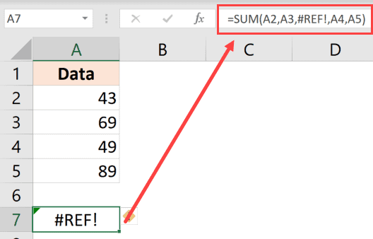
You can see that the third argument in the formula has become #REF! (which earlier referred to the cell that we deleted).
Take away / How to Fix: Before you delete any data that is being used in formulas, make sure there are no errors after the deletion. It’s also recommended that you create a backup of your work regularly to make sure you always have something to fall back on.
Incorrect Placement of Parenthesis (BODMAS)
As your formulas start to get bigger and more complex, it’s a good idea to use parenthesis to be absolutely clear of what part belongs together.
In some cases, you may have the parenthesis at the wrong place, which can either give you a wrong result or an error.
And in some cases, it’s recommended to uses parenthesis to make sure the formula understands what needs to be grouped and calculated first.
For example, suppose you have the following formula:
=5+10*50
In the above formula, the result is 505 as Excel first does the multiplication and then the addition (as there is an order of precedence when it comes to operators).
If you want it to first do the addition and then the multiplication, you need to use the below formula:
=(5+10)*50
In some cases, the order of precedence may work for you, but it’s still recommended that you use the parenthesis to avoid any confusion.
Also, in case you’re interested, below is the order of precedence for various operators often used in formulas:
| Operator | Description | Order of Precedence |
| : (colon) | Range | 1 |
| (single space) | Intersection | 2 |
| , (comma) | union | 3 |
| – | Negation (as in –1) | 4 |
| % | Percentage | 5 |
| ^ | Exponentiation | 6 |
| * and / | Multiplication & division | 7 |
| + and – | Addition & subtraction | 8 |
| & | Concatnenation | 9 |
| = < > <= >= <> | Comparison | 10 |
Take away / How to Fix: Always use parenthesis to avoid any confusion, even if you know the order of precedence and are using it correctly. Having parenthesis makes it easier to audit formulas.
Incorrect Use of Absolute/Relative Cell References
When you copy and paste formulas in Excel, it automatically adjusts the references. Sometimes, this is exactly what you want (mostly when you’re copy-pasting formulas down the column), and sometimes you don’t want this to happen.
An absolute reference is when you fix a cell reference (or range reference) so that it doesn’t change when you copy and paste formulas, and a relative reference is one that changes.
You can read more about absolute, relative, and mixed references here.
You may get an incorrect result in case you forget to change the reference to an absolute one (or vice versa). This is something that happens quite often to me when I am using lookup formulas.
Let me show you an example.
Below I have a dataset where I want to fetch the score in Exam 1 for the names in column E (a simple VLOOKUP use case)

Below is the formula that I use in cell F2 and then copies to all the cells below it:
=VLOOKUP(E2,A2:B6,2,0)

As you can see that this formula gives an error in some cases.
This happens because I haven’t locked the table array argument – it’s A2:B6 in cell F2, while it should have been $A$2:$B$6
By having these dollar signs before the row number and column alphabet in a cell reference, I am forcing Excel to keep these cell references fixed. So, even when I copy this formula down, the table array will continue to refer to A2:B6
Pro Tip: To convert a relative reference to an absolute one, select that cell reference within the cell, and press the F4 key. You would notice that it changes by adding the dollar signs. You can continue to press F4 until you get the reference you want.
Incorrect Reference to Sheet / Workbook Names
When you refer to other sheets or workbooks in a formula, you need to follow a specific format. And in case the format is incorrect, you will get an error.
For example, if I want to refer to cell A1 in Sheet2, the reference would be =Sheet2!A1 (where there is an exclamation sign after the sheet name)
And in case there are multiple words in the sheet name (let’s say it’s Example Data), the reference would be =’Example Data’!A1 (where the name is enclosed in single quotes followed by an exclamation sign).
In case you’re referring to an external workbook (let’s say you’re referring to cell A1 in ‘Example Sheet’ in the workbook named ‘Example Workbook’), the reference will be as shown below:
='[Example Workbook.xlsx]Example Sheet'!$A$1
And in case you close the workbook, the reference would change to include the entire path of the workbook (as shown below):
='C:UserssumitDesktop[Example Workbook.xlsx]Example Sheet'!$A$1
In case you end up changing the name of the workbook or the worksheet to which the formula refers to, it’s going to give you a #REF! error.
Also read: How to Find External Links and References in Excel
Circular References
A circular reference is when you refer (directly or indirectly) to the same cell where the formula is being calculated.
Below is a simple example, where I use the SUM formula in cell A4 while using it in the calculation itself.
=SUM(A1:A4)
Although Excel shows you a prompt letting you know about the circular reference, it will not do it for every instance. And this may give you the wrong result (without any warning).
In case you suspect circular reference in play, you can check which cells have it.
To do this, click the Formula tab and in the ‘Formula Auditing’ group, click on the Error Checking drop-down icon (the small downward pointing arrow).
Hover the cursor over the Circular reference option and it will show you the cell that has the circular reference issue.

Cells Formatted as Text
If you find yourself in a situation where as soon as you type the formula as hit enter, you see the formula instead of the value, it’s a clear case of the cell being formatted as text.

When a cell is formatted as text, it considers the formula as a text string and shows it as is.
It doesn’t force it to calculate and give the result.
And it has an easy fix.
- Change the format to ‘General’ from ‘Text’ (it’s in Home tab in the Numbers group)
- Go to the cell that has the formula, get into the edit mode (use F2 or double click on the cell) and hit Enter
In case the above steps don’t solve the problem, another thing to check is whether the cell has an apostrophe at the beginning. A lot of people add an apostrophe to convert formulas and numbers to text.
If there is an apostrophe, you can simply remove it.
Text Automatically Getting Converted into Dates
Excel has this bad habit of converting that looks like a date into an actual date. For example, if you enter 1/1, Excel would convert it to 01-Jan of the current year.
In some cases, this may be exactly what you want, and in some cases, this may work against you.
And since Excel stores date and time values as numbers, as soon as you enter 1/1, it converts it into a number representing the January 1 of the current year. In my case, when I do this, it converts it into the number 43831 (for 01-01-2020).
This could mess with your formulas if you’re using these cells as an argument in a formula.
How to fix this?
Again, we don’t want Excel to automatically pick the format for us, so we need to clearly specify the format ourselves.
Below are the steps to change the format to text so that it doesn’t automatically convert text to dates:
- Select the cells/range where you want to change the format
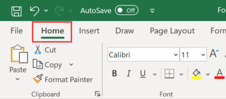
- Click on the Home tab

- In the Number group, click on the Format drop-down
- Click on Text


Now, whenever you enter anything in the selected cells, it would be considered as text, and not changed automatically.
Note: The above steps would only work for data entered after the formatting has been changed. It will not change any text that has been converted to date before you made this formatting change.
Another example where this can be really frustrating is when you enter a text/number that has leading zeros. Excel automatically removes these leading zeros as it considers these useless. For example, if you enter 0001 in a cell, Excel will change it to 1. In case you want to keep these leading zeros, use the steps above.
Hidden Rows/Columns Can Give Unexpected Results
This is not a case of formula giving you the wrong result but of using the wrong formula.
For example, suppose you have a dataset as shown below and I want to get the sum of all the visible cells in column C.

In cell C12, I have used the SUM function to get the total sale value for all these given records.

So far so good!
Now, I apply a filter to the item column to only show the records for Printer sales.

And here is the problem – the formula in cell C12 still shows the same result – i.e., the sum of all the records.
As I said, the formula is not giving the wrong result. In fact, the SUM function is working just fine.
The issue is that we have used the wrong formula here.
SUM function can not account for the filtered data and give you the result for all the cells (hidden or visible). If you only want to get the sum/count/average of visible cells, use SUBTOTAL or AGGREGATE functions.
Key takeaway – Understand the correct use and limitations of a function in Excel.
These are some of the common causes that I have seen where your Excel formulas may not work or give unexpected or wrong results. I am sure there are many more reasons for an Excel formula to not work or update.
In case you know of any other reason (maybe something that irks you often), let me know in the comments section.
Hope you found this tutorial useful!
You may also like the following Excel tutorials:
- How to Lock Formulas in Excel
- How to Copy and Paste Formulas in Excel without Changing Cell References
- Show Formulas in Excel Instead of the Values
- Convert Text to Numbers in Excel
- Convert Date to Text in Excel
- Microsoft Excel Won’t Open; How to Fix it!
- Arrow Keys not Working in Excel | Moving Pages Instead of Cells
- 20 Advanced Excel Functions and Formulas
If you have had problems where the Excel formulas don’t work.So this post is for you!
Anyone who uses formulas in Excel will sooner or later run into the problem that the formulas don’t work (or give the wrong result). Unfortunately, when it comes to Excel formulas, there are many things that can go wrong. But the good news is that if you go through some common causes, you will probably solve most of the problems where formulas don’t work in Excel.
In this article, we’ll show you the main issues that are likely causing your Excel formulas not to work. Verify!
Excel formulas not working: main reasons
Browse the topic of your interest:
Incorrect use of function syntax
Every function in Excel has a specific syntax that contains the number of arguments it can take or the type of arguments it can accept.
And in many cases, the reason why your Excel formulas are not working or giving the wrong result could be a wrong argument (or missing arguments).
For example, the VLOOKUP function takes three required arguments and one optional argument.
If you provide the wrong argument or don’t specify the optional argument (where it is required for the formula to work), it will return an incorrect result.
For example, suppose you have a table like the one shown in the image below, and you want to use the VLOOKUP function to get the grade for a particular student in cell E2. Note that you will need to specify the argument lookup valuewhich in this case is the name of the student.
On the other hand, if you don’t specify this argument, the formula will return the error #N/A.

So in this case, just enter a valid student name in cell D2 for the function to return the correct result.
See also the following article: Learn the VLOOKUP function in less than 2 minutes
Use of extra spaces
Leading and trailing spaces are hard to figure out and can cause problems when you use a cell that has them in formulas.
For a better understanding, take a look at the example below where we are using the PROCV function to get the grade for the student Carlos. However, the result of the formula is the #N/A error (not available error).

Although the formula is correct and the name ‘Carlos’ clearly exists in the list, what we can’t see is that there is a trailing space in the cell that has the name (in cell D2).

Excel does not consider the contents of these two cells to be the same, and therefore considers a discrepancy when getting the value using VLOOKUP (or any other lookup formula).
To fix this problem, you must remove these extra space characters. You can do this using any of the following methods:
1. Clear cell and remove leading/trailing spaces before using it in formulas
two. Use the TILE function in the formula to ensure that leading, trailing, or double spaces are ignored. For more details on this tip, see the article: How to remove blank spaces in Excel
Use of manual calculation instead of automatic
Another common reason why Excel formulas don’t work is the use of manual calculations instead of automatic ones.
This setting may drive many Excel users crazy, because what few people know is that Excel has two calculation modes: Automatic and Manual.
By default, automatic mode is enabled, which means that if you use a formula or make any changes to existing formulas, it will automatically (and instantly) do the calculation and give me the result.
However, in some cases, Excel users enable the manual calculation setting. This is usually done when you have a large Excel file with lots of data and formulas. In these cases, you may not want Excel to recalculate everything when you make small changes (as it can take a few seconds or even minutes) for this recalculation to complete.
If you enable manual calculation, Excel won’t calculate unless you force it, making you think your formula isn’t working correctly. In this case, all you need to do in this case is to set the calculation back to automatic or force a recalculation by pressing the F9 key.
Below are the steps to change the calculation from manual to automatic:
1. access the guide formulas
two. click on Calculation Optionsor and select Automatic

Rows or columns deleted
Another reason your Excel formulas may not work is the exclusion of rows or columns that are used in calculations.
When this happens, Excel can sometimes adjust the reference and make sure the formulas continue to work correctly. However, this is not always possible.
A clear indication you get when formulas fail to delete cells/rows/columns is the #REF error! in cells This is a reference error that tells you there is a problem with the references in the formula.
For a better understanding, consider the following example where we are using the SUM function to add the values in the range A1:A6

Now, if we delete any of those cells/rows, the SUM formula will return the #REF! error. This happens because when we delete the row, the formula doesn’t know what to reference.

In the image above, notice that the third argument of the formula has been converted to #REF. (which previously referred to the cell we deleted).
To work around this problem, before deleting data that is used in formulas, make sure there are no errors after deletion. It is also recommended that you back up your work regularly to ensure that you always have something to fall back on.
Incorrect use of parentheses.
As your formulas start to get larger and more complex, it is recommended that you use parentheses to make it absolutely clear which part to join. In some cases, you may have the parentheses in the wrong place, which may give the wrong result or error.
For example, suppose you have the following formula:
=10+12*50
In the above formula, the result is 610 since Excel does the multiplication first and then the addition (since there is an order of precedence when it comes to operators).
If you want to do the addition first and then the multiplication, you should use the following formula:
=(10+12)*50
In some cases, the order of precedence may work for you, but it is still recommended that you use parentheses to avoid confusion.
Incorrect use of absolute/relative cell references
When you copy and paste formulas into Excel, it automatically adjusts the references. Sometimes this is exactly what you want (especially when you’re copying and pasting formulas into the column), but sometimes you don’t want it to happen.
An absolute reference is when you set a cell reference (or range reference) so that it doesn’t change when you copy and paste formulas, and a relative reference is one that changes.
For more information on this topic, see the article: Cell references: relative, absolute and mixed
You may get an incorrect result if you forget to change the reference to an absolute (or vice versa). For a better understanding, please take a look at the example below where we are using the VLOOKUP function to return the grades of all students in column E. The formula was inserted into cell E2 and then we used the Excel fill handle to apply the formula to the other cells.

However, as you can see, the formula has an error in some cases. This happens because we don’t block the table_array argument — it is A2: B6 in cell D2, while it should be $A$2:$B$6
By having these dollar signs before the row number and column alphabet in a cell reference, I am forcing Excel to keep these cell references fixed. So even when I copy this formula, the table array will still refer to A2:B6.
So before you drag your formula into more cells, make sure the references are correct. To convert a relative reference to an absolute reference, select that cell reference within the cell and press the F4 key. You’ll notice this changes as you add the dollar signs. You can keep pressing F4 until you get the reference you want.

Using wrong reference to worksheet/workbook names
When referring to other worksheets or workbooks in a formula in Excel, you must follow a specific format. And in case the format is wrong, you will get an error.
For example, if I want to reference cell A1 on Sheet2, the reference would be =Sheet2!A1 (where there is an exclamation point after the sheet name).
And if there are multiple words in the spreadsheet name (for example: Monthly Billing 2022), the reference would be =’Monthly billing 2022′!A1 (where the name is enclosed in single quotes followed by an exclamation mark).
In case you are referring to an external workbook (let’s say you are referring to cell A1 in ‘Monthly Invoicing 2022’ in the workbook named ‘Sales Control’), the reference will be as shown below:
='[Monthly Billing 2022.xlsx]Monthly Billing 2022'!$A$1
And in case you close the workbook, the reference will change to include the full path of the workbook (as shown below):
='C:UsersExcelEasyDesktop[Monthly Billing 2022.xlsx]Monthly Billing 2022'!$A$1
If you end up changing the name of the workbook or sheet that the formula references, it will return the #REF! error.
Circular references
A circular references They are also often common reasons why Excel formulas don’t work.
A circular reference is when you refer (directly or indirectly) to the same cell where the formula is calculated.
Below is a simple example where we are using the SUM function on cell A5 while using it in the calculation itself.
= SUM (A1: A5)
Although Excel will tell you about the circular reference, it won’t always do so. And it might give you wrong result (without warning). And if you suspect a circular reference in your formulas, you can check which cells have it.
To do this, go to the tab Formula and in the group Formula Auditclick the dropdown icon Error checking (the little arrow pointing down).
Hover over the option Circular references and it will show the cell that has the circular reference problem.

Cells formatted as Text
If you entered a formula into a cell in Excel and pressing Enter returned the formula instead of the value, then it is a clear case that the cell is formatted as text.

When a cell is formatted as text, Excel considers the formula to be a text string and displays it as is. In this case, you will have two possible solutions:
1. Change cell format to General instead of Text.
two. Go to the cell that has the formula, enter edit mode (use F2 or double-click the cell), and press Enter
If the above steps don’t resolve the issue, another thing to check is if the cell has an apostrophe at the beginning. Many people add an apostrophe to convert formulas and numbers to text. If there is an apostrophe, you can simply remove it.
Also check out the following Excel tips:
So what do you think of the tips? Now, whenever you notice that your Excel formulas are not working, just come back to this article and check each topic to find the solution.
Bottom Line: Learn about the different calculation modes in Excel and what to do if your formulas are not calculating when you edit dependent cells.
Skill Level: Beginner
Watch the Tutorial
Download the Excel File
You can follow along using the same workbook I use in the video. I’ve attached it below:
Why Aren’t My Formulas Calculating?
If you’ve ever been in a situation where the formulas in your spreadsheet are not automatically calculating as they should, you know how frustrating it can be.
This was happening to my friend Brett. He was telling me that he was working with a file and it wasn’t recalculating the formulas as he was entering data. He found that he had to edit each cell and hit Enter for the formula in the cell to update.
And it was only happening on his computer at home. His work computer was working just fine. This was driving him crazy and wasting a lot of time.
The most likely cause of this issue is the Calculation Option mode, and it’s a critical setting that every Excel user should know about.
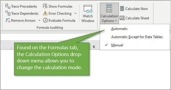
To check what calculation mode Excel is in, go to the Formulas tab, and click on Calculation Options. This will bring up a menu with three choices. The current mode will have a checkmark next to it. In the image below, you can see that Excel is in Manual Calculation Mode.
When Excel is in Manual Calculation mode, the formulas in your worksheet will not calculate automatically. You can quickly and easily fix your problem by changing the mode to Automatic. There are cases when you might want to use Manual Calc mode, and I explain more about that below.
Calculation Settings are Confusing!
It’s really important to know how the calculation mode can change. Technically, it’s is an application-level setting. That means that the setting will apply to all workbooks you have open on your computer.
As I mention in the video above, this was the issue with my friend Brett. Excel was in Manual calculation mode on his home computer and his files weren’t calculating. When he opened the same files on his work computer, they were calculating just fine because Excel was in Automatic calculation mode on that computer.
However, there is one major nuance here. The workbook (Excel file) also stores the last saved calculation setting and can change/override the application-level setting.
This should only happen for the first file you open during an Excel session.
For example, if you change Excel to manual calc mode before you save & close the file, then that setting is stored with the workbook. If you then open that workbook as the first workbook in your Excel session, the calculation mode will be changed to manual.
All subsequent workbooks that you open during that session will also be in manual calculation mode. If you save and close those files, the manual calc mode will be stored with the files as well.
The confusing part about this behavior is that it only happens for the first file you open in a session. Once you close the Excel application completely and then re-open it, Excel will return to automatic calculation mode if you start by opening a new blank file or any file that is in automatic calculation mode.
Therefore, the calculation mode of the first file you open in an Excel session dictates the calculation mode for all files opened in that session. If you change the calculation mode in one file, it will be changed for all open files.
Note: I misspoke about this in the video when I said that the calculation setting doesn’t travel with the workbook, and I will update the video.
The 3 Calculation Options
There are three calculation options in Excel.
Automatic Calculation means that Excel will recalculate all dependent formulas when a cell value or formula is changed.
Manual Calculation means that Excel will only recalculate when you force it to. This can be with a button press or keyboard shortcut. You can also recalculate a single cell by editing the cell and pressing Enter.
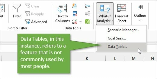
Automatic Except for Data Tables means that Excel will recalculate automatically for all cells except those that are used in Data Tables. This is not referring to normal Excel Tables that you might work with frequently. This refers to a scenario-analysis tool that not many people use. You find it on the Data tab, under the What-If Scenarios button. So unless you’re working with those Data Tables, it’s unlikely you will ever purposely change the setting to that option.
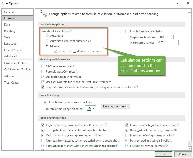
In addition to finding the Calculation setting on the Data tab, you can also find it on the Excel Options menu. Go to File, then Options, then Formulas to see the same setting options in the Excel Options window.
Under the Manual Option, you’ll see a checkbox for recalculating the workbook before saving, which is the default setting. That’s a good thing because you want your data to calculate correctly before you save the file and share it with your co-workers.
Why Would I Use Manual Calculation Mode?
If you are wondering why anyone would ever want to change the calculation from Automatic to Manual, there’s one major reason. When working with large files that are slow to calculate, the constant recalculation whenever changes are made can sometimes slow your system. Therefore people will sometimes switch to Manual mode while working through changes on worksheets that have a lot of data, and then will switch back.
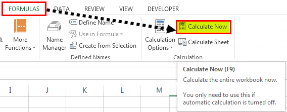
When you are in Manual Calculation mode, you can force a calculation at any time using the Calculate Now button on the Formulas tab.
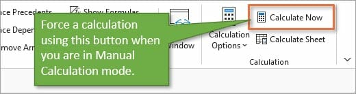
The keyboard shortcut for Calculate Now is F9, and it will calculate the entire workbook. If you want to calculate just the current worksheet, you can choose the button below it: Calculate Sheet. The keyboard shortcut for that choice is Shift + F9.
Here is a list of all Recalculate keyboard shortcuts:
| Shortcut | Description |
| F9 | Recalculate formulas that have changed since the last calculation, and formulas dependent on them, in all open workbooks. If a workbook is set for automatic recalculation, you do not need to press F9 for recalculation. |
| Shift+F9 | Recalculate formulas that have changed since the last calculation, and formulas dependent on them, in the active worksheet. |
| Ctrl+Alt+F9 | Recalculate all formulas in all open workbooks, regardless of whether they have changed since the last recalculation. |
| Ctrl+Shift+Alt+F9 | Check dependent formulas, and then recalculate all formulas in all open workbooks, regardless of whether they have changed since the last recalculation. |
Macro Changing to Manual Calculation Mode
If you find that your workbook is not automatically calculating, but you didn’t purposely change the mode, another reason that it may have changed is because of a macro.
Now I want to preface this by saying that the issue is NOT caused by all macros. It’s a specific line of code that a developer might use to help the macro run faster.
The following line of VBA code tells Excel to change to Manual Calculation mode.
Application.Calculation = xlCalculationManual
Sometimes the author of the macro will add that line at the beginning so that Excel does not attempt to calculate while the macro runs. The setting should then changed be changed back at the end of the macro with the following line.
Application.Calculation = xlCalculationAutomatic
This technique can work well for large workbooks that are slow to calculate.
However, the problem arises when the macro doesn’t get to finish—perhaps due to an error, program crash, or unexpected system issue. The macro changes the setting to Manual and it doesn’t get changed back.
As I mention in the video, this was exactly what happened to my friend Brett, and he was NOT aware of it. He was left in manual calc mode and didn’t know why, or how to get Excel calculating again.
Therefore, if you are using this technique with your macros, I encourage you to think about ways to mitigate this issue. And also warn your users of the potential of Excel being left in manual calc mode.
I also recommend NOT changing the Calculation property with code unless you absolutely need to. This will help prevent frustration and errors for the users of your macros.
Conclusion
I hope this information is helpful for you, especially if you are currently dealing with this particular issue. If you have any questions or comments about calculation modes, please share them in the comments.
An Excel formula not working is a type of Excel formula error. This issue occurs when the formula returns an incorrect result or an error value instead of the calculated results.
Typically, users face an Excel formula not working when they enter it with syntax or input values’ format issues or incorrect arguments. The problem might also occur when working with multiple workbooks containing a large amount of data and formulas.
For example, the below image shows two tables. The first table contains the subject scores of 10 students.

Select cell H2, and enter the VLOOKUP() formula =VLOOKUP(G2,A:C,3,0,FALSE) to display the Physics score of the student specified in cell G2 in the second table.

- Error/Warning → We get the error that we entered too many arguments.
- Reason → The entered VLOOKUP excel function contains one additional argument.
- Correct formula → =VLOOKUP(G2,A:C,3,FALSE) Or =VLOOKUP(G2,A:C,3,0)
- Right Output: We will get the correct Physics score of the specified student, Lisa Maxwell, 98.
- Error Observation and Solution: Thus, we can avoid such a case of the Excel formula not working warning by checking if the entered formula or function contains all the required arguments.
Table of contents
- What Is Excel Formula Not Working?
- Top 10 Reasons (with Solutions)
- #1 – Mismatch in Opening and Closing Parentheses in a Function/Formula
- #2 – Function Arguments not Seperated with the Required Character
- #3 – All Required Function Arguments Not Provided
- #4 – Incorrect Function Syntax
- #5 – A Number Value in an Excel Formula is in Double Quotations or Text Format
- #6 – Number Values Entered with Formatting
- #7 – Using Absolute Reference Incorrectly
- #8 – Nesting More Than 64 Functions in an Excel Formula
- #9 – Workbook or Worksheet Names in a Formula Not Enclosed in Single Quotations
- #10 – Full Path of Closed Workbook Not Provided while Referring to It in the Formula
- Why Excel Formulas Not Updating?
- Why Excel Formulas Not Calculating?
- #1 – Show Formula Mode is On
- #2 – The Formula Entered as a Text
- #3 – The Target cell Formula Has a Leading Space or Apostrophe Before the ‘=’ Sign
- Important Things to Note
- Frequently Asked Questions (FAQs)
- Download Template
- Recommended Articles
- Top 10 Reasons (with Solutions)
- The Excel formula not working is an Excel formula error condition, where the specific formula returns a warning/error message or an incorrect value.
- Users might find Excel formula not working when their worksheets contain massive datasets involving formulas. They might also face the issue when referring to multiple workbooks and worksheets in the active spreadsheet.
- If the Excel formulas do not update automatically, check the Calculation Options setting in the Formulas tab. It should be Automatic.
- If we find the Excel formulas not calculating, check for the following causes:
- Show Formulas mode is On.
- The entered formula is in the Text format.
- The entered formula contains a leading space or apostrophe before the ‘=’ sign.
Top 10 Reasons (with Solutions)
We will consider the Top 10 reasons for the Excel formula not working and the solutions.
#1 – Mismatch in Opening and Closing Parentheses in a Function/Formula
Typically, complex Excel formulas include multiple sets of opening and closing parentheses. They help define the order of the calculations within the formula.
However, if we enter an opening parenthesis but miss its matching closing parenthesis or vice versa in a formula, we may have the scenario of the Excel formula not working.
For example, the first table in the image below shows a list of items and their order details.

To determine the order status for the item specified in the second table based on the units required and ordered data in the first table, select cell F2, and enter the formula =IF((VLOOKUP(E2,A:C,3,0)>VLOOKUP(E2,A:B,2,0)),”Order Fulfilled”,”Order Unfulfilled” as shown below.

However, on applying the formula, we get the above warning message. The reason is the opening and closing parentheses mismatch. Excel identifies it as a typo error and suggests correcting the issue. In this case, the formula is missing the last closing parenthesis. So, we can click Yes in the error message window or close the window and manually enter the last closing parenthesis to get the correct result.

Solution
We can check the following points to avoid such a condition of the Excel formula not working.
- Excel highlights each opening and closing parenthesis pair in a different color. We can check the colors to locate the missing or additional parenthesis.
- While entering the closing parenthesis, Excel will momentarily make its opening parenthesis pair bold. And if it does not show the matching opening parenthesis in bold, it indicates a mismatch.
- When we click the Formula Bar or double-click the cell containing the formula, Excel shows the opening and closing parenthesis pair in the respective colors. We can use the color code to check for the missing parenthesis.
#2 – Function Arguments not Seperated with the Required Character
We might have an Excel formula not working if we do not use the required list separator in the formula properly.
For example, once again, consider the previous example. If we enter the formula as depicted in the image below, we will have the condition of the Excel formula not working.

The IF excel function is missing the list separator, ‘,’ between the TRUE and FALSE values.
However, if we do not use a list separator according to our Excel regional settings, our Excel formulas might also not work in such a scenario.
For example, the formula, =IF((VLOOKUP(E2,A:C,3,0)>VLOOKUP(E2,A:B,2,0)),”Order Fulfilled”,”Order Unfulfilled”) might not work in European countries, as they consider a ‘;’ as a list separator, while the ‘,’ works in North America.
Solution
- Confirm whether we included the list separator at every required position in the formula before executing it.
For example, in the above IF(), once we enter the list separator, ‘,’, between the TRUE and FALSE values, the function will return the correct result.

- Go to Control Panel → Region and Language → Additional Settings to check the Regional Settings and the accepted List Separator character. And then ensure we use the applicable list separator in our Excel formulas.
#3 – All Required Function Arguments Not Provided
Typically, an Excel function requires mandatory arguments. However, some also include optional arguments for which the functions take the default values if not provided.
But when we provide only some of the mandatory arguments to the specific formula, we will have the scenario of the Excel formula not working.
For example, the following table contains the mandatory arguments required to compute the compound interest in cell B8.

But when we enter the FV excel function in the target cell B8 to get the compound interest, as depicted in the image below, we will get the Excel formula not working.

The warning message says the entered arguments are too few for this function. And if we enter more than the required arguments, Excel returns a warning message for such issues, stating the entered arguments are too many for this function.
Solution
We can enter the Excel formula in two ways, which will help us avoid this situation.
- Enter the formula directly in the target cell. Once we enter the ‘=’ symbol and the function name, Excel will show the mandatory and optional arguments we need to provide to execute it. For example, in the above table, we will see the FV formula syntax.

Excel will highlight the argument to enter.

And finally, when we close the parenthesis and press Enter, the formula will get executed.

- We can use the function from the Formulas tab, which allows us to enter the arguments in the Function Arguments window. It will ensure that we enter all the required arguments. For example, the FV() is a Financial formula in the Formulas tab. So, we can select the target cell and navigate as depicted below to enter the arguments in the Function Arguments window.

The Function Arguments window opens, showing the mandatory argument names in bold.
Enter the mandatory arguments correctly in the window and click OK, as shown below.

The formula executed gives the following output.

#4 – Incorrect Function Syntax
When we enter a function with incorrect syntax, it can lead to the Excel formula not working.
For example, if we enter the function name incorrectly in the previous example, the formula will not work.

The entered function is FB() instead of FV(). Thus, the function returns the #NAME? error.
Likewise, the last optional argument in the FV() can take a value of 0 or 1. Or we can enter the argument value as FALSE or TRUE without double quotes. And if we enter the last argument, Type, as a value other than the mentioned options, it will result in the Excel formula not working.

In the above example, the last argument value is in double quotes, leading to the function returning the #VALUE! error.
Solution
- Ensure we enter the correct Excel function or the required formula.
- Check the function or formula syntax for correct argument values before executing the function.
For example, we will get the required output when correctly entering the last argument value without the double quotes in the above FV().

#5 – A Number Value in an Excel Formula is in Double Quotations or Text Format
When we enter a number value in a formula but within double quotes or in the text format, it leads to the Excel formula not working.
For example, the first table contains a list of values. And the second table shows two conditions to get the required results.

Select cell E2, and enter the IF() formula to achieve the desired outcome.

The cell E2 shows the correct result, 1, as the sum of all the values in the first table is 15, a value greater than 4. Unfortunately, Excel treats the function return value as a text string. And thus, we cannot use it in other Excel functions to perform calculations.
On the other hand, if the provided values in the first table are in text format. And we use them in an Excel function to perform the required calculations. Then, it will lead to the Excel function not working.
For example, the first table values are in Text format, as the Number Format in the Home tab shows the cells’ data format as Text.

Now, if we use the first table values in the SUM excel function in the cell E3, the output will be:

While the correct result is 15, since all the number values in the first table are in text format, the SUM() considers them as text values and thus returns an incorrect output, 0.
Also, in such conditions, the Status Bar showing only the function COUNT indicates that the worksheet contains many number values in text format. Otherwise, we should be able to see other Excel functions, such as SUM and AVERAGE.
Solution
- Ensure we do not provide number values in double quotations to an Excel function.
- If we see number values left-aligned in cells, check the Number Format option in the Home tab and change the format from Text to General or Number.

However, if the issue persists even after changing the Number Format, delete the data and enter the values again with the Number Format being General or Number.
- We can select all the error cells, click the error message and choose the option Convert to Number.

And once we choose the option mentioned above, the SUM() in cell E3 will return the correct value.

#6 – Number Values Entered with Formatting
When we enter numbers with formatting such as Currency while typing a formula, we may end up with the Excel formula not working.
For example, the below table shows a list of items, their prices per unit, and the number of units ordered.

To find the total value of the order in $ for each item to display the result in column D, we will apply the above-shown formulas in column D, with a ‘$’ symbol before the column B values, as we want to display the result as currency values. However, the resulting amounts in column D are not currency values.
Solution
- Avoid using a decimal separator or currency sign, such as ‘$’, while entering a number in an Excel function to avoid the scenario of the Excel formula not working. The reason is, typically, commas separate function arguments, and the ‘$’ symbol before a cell reference makes it an absolute cell reference.
- After entering the number as a plain number, right-click the cell and choose the Format Cells option from the contextual menu to apply the required formatting.
For example, remove the ‘$’ symbol in the column D formulas in the above table.

Then, use the Format Cells option, as explained above, to get the required result.

The “Format Cells” window appears.

The “Number Format” is now changed to “Currency”.

#7 – Using Absolute Reference Incorrectly
When we do not properly use absolute references in a function, it might lead to the Excel formula not working.
For example, the first table shows a list of students, their admission numbers, and grade details.

The second table contains the same list of students but in alphabetical order, and we have to update their grades using the data in the first table. So, we will apply the VLOOKUP() in the target cells without using the absolute reference for the lookup range to get the following output.

The issue is the lookup range in the VLOOKUP() has to be the same in all the target cells. But, as the VLOOKUP() applied in the first target cell does not use the absolute reference to the lookup range, the range changes when we copy the VLOOKUP() in the following cells. It thus leads to the Excel formula not working in each cell that falls outside the lookup range.
Solution
- Make the required cell reference absolute in the formulas to use the same cell value in the specific target cells’ functions.
For example, once we provide the absolute cell reference to the lookup range in the above VLOOKUP functions, the range remains the same in all the target cells. And the output will be:

#8 – Nesting More Than 64 Functions in an Excel Formula
When applying Excel formulas such as the Nested IF function, we might nest more than 64 functions in the formula to meet our requirement. However, such a scenario will lead to the Excel formula not working.
The reason is that the maximum nesting capacity in Excel version 2007 and above is 64. On the other hand, the function nesting capacity in Excel versions before 2007 is 7.
Solution
- If our Excel version is 2007 or above, ensure we use up to 64 levels of nested functions.
- If our Excel version is before 2007, we can have the maximum nested function level of 7.
#9 – Workbook or Worksheet Names in a Formula Not Enclosed in Single Quotations
To refer to other worksheets or workbooks in our formula, but their names contain spaces or non-alphabetic characters, we must enclose their names in single quotations to avoid the scenario of the Excel formula not working.
The below image shows two tables. And is we need to update the first and second tables using data from another workbook and a worksheet in the current worksheet.

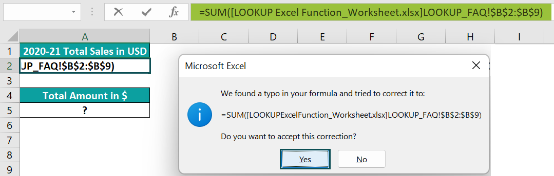
- Select cell A2, and enter the formula =SUM([LOOKUP Excel Function_Worksheet.xlsx]LOOKUP_FAQ!$B$2:$B$9)
[Note: The workbook name contains spaces, and as we did not enclose the name in single quotations, we see the above warning message.]

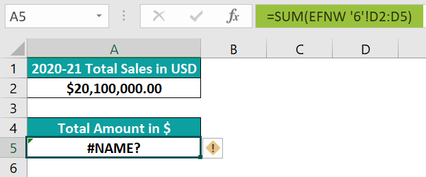
- Select cell A5, and enter the formula =SUM(EFNW ‘6′!D2:D5)
[Note: The single quotations do not enclose the entire worksheet name containing a space. And thus, Excel does not recognize the worksheet name and returns the #NAME? error.]

Solution
- Enter the formula with the workbook name in single quotations to get the required data,
as =SUM(‘[LOOKUP Excel Function_Worksheet.xlsx]LOOKUP_FAQ’!$B$2:$B$9)

- Enclose the entire worksheet name in single quotations to achieve the desired results,
as =SUM(‘EFNW 6’!D2:D5)

#10 – Full Path of Closed Workbook Not Provided while Referring to It in the Formula
When referring to another closed workbook in a formula, the external reference should include the entire path to the workbook.
For example, cell A2 contains a formula that refers to a closed workbook. And if we do not provide the entire path to the workbook, it might lead to the Excel formula not working.

Solution
- When referencing a closed workbook in a formula, ensure we include the entire path to the workbook and its name in the external reference.

Why Excel Formulas Not Updating?
Sometimes, the formula does not return the updated value automatically. Instead, it shows the previous result, even after updating the required cell references.
For example, the table below shows the monthly savings calculations in column D.

However, even when the formulas in cells D3:D7 contain the respective dependent cells’ references, the output in every cell in column D remains the same, cell D2 result.
The reason is that the Calculation Options setting is not Automatic. Instead, it is Manual.

Solution
- Set the Calculation settings as Automatic
Go to the File tab.

Choose the Options option.

Next, click the Formulas tab in the menu and set the Calculation options as Automatic.

The target cells will automatically get updated with the correct function return values.

- If we want the Calculation Options to be Manual and to recalculate the entire Excel workbook, we can force the calculation using the shortcut keys F9 or Formulas → Calculate Now.

And if we need to recalculate an active worksheet, press the shortcut keys Shift + F9 or use Formulas → Calculate Sheet.

On the other hand, by pressing Ctrl + Alt + F9, we can recalculate all the worksheets in all the open workbooks. But if we need to recalculate a single formula in a worksheet, select the specific cell with the formula and enter the edit mode. We can do so by pressing the F2 key or double-clicking the specific cell. And finally, press Enter to execute the formula.
Why Excel Formulas Not Calculating?
When we enter a formula in a cell, the cell displays the formula instead of the formula’s calculated value. Then, check for the below issues to ensure the formula works.
- Show Formulas Mode Is On.
- The Formula Entered as A Text.
- The Target Cell Formula Has A Leading Space or Apostrophe Before The ‘=’ Sign.
Let us understand in detail and look into the workaround.
#1 – Show Formula Mode is On
When we enter the required formulas in column B in the table below, the target cells show the entered formulas instead of their return values.
The reason is the Show Formulas mode in the Formulas tab is ON.

Solution
- Ensure the Show Formulas mode is OFF to view the formula return values. And for that, we can press Ctrl + ` or unselect the Show Formulas option in the Formulas tab.

#2 – The Formula Entered as a Text
Considering the previous example, if the target cells display the entered formulas instead of their return values, we must check the target cells’ Number Format in the Home tab. If it is Text, it could be the reason for this issue.

Solution
- Set the target cell’s Number Format in the Home tab as General.

The “Number Format” is now in “General” format.

And then, select cell B2 and press F2 to go to the edit mode.

Next, press Enter to recalculate the formula and get its return value.

Finally, repeat the above steps to recalculate the formulas in cells D3:D6 or use the fill handle to copy the cell D2 formula in cells D3:D6.

#3 – The Target cell Formula Has a Leading Space or Apostrophe Before the ‘=’ Sign
Continuing with the previous example, if we enter the required formula in cell B2 but with a leading space or an apostrophe in front of the ‘=’ sign, then we will see the formula in the target cell and not its evaluated value, as shown in the images below.


Solution
- When entering a formula in the target cell, ensure we do not enter a leading space or an apostrophe before the ‘=’ sign. And when copying a formula from the web, ensure there is no space before the ‘=’ sign.

Important Things to Note
- While applying the formula in a cell, ensure the function syntax is correct, with the correct number of matching parentheses and appropriate list separators. Also, check if we have entered the values for all the mandatory arguments to the function. Otherwise, it might lead to the Excel formula not working.
- Do not enter numbers in the formulas as text values or within double quotations.
- Use absolute references properly, and do not nest more than 64 functions in a formula.
Frequently Asked Questions (FAQs)
1. What are the different types of Excel formula errors?
Some of the Excel formula errors are as follows:
• The Excel formula is not working.
• The Excel formula is not updating.
• Excel formula not calculating.
• Too many arguments entered in the formula or too few arguments without the mandatory argument values.
2. Can an incorrect cell format lead to the Excel formula not working?
An incorrect cell format can lead to the Excel formula not working, specifically if it’s a Text format.
For example, the table below shows the length and breadth values of a rectangle. And column C contains the formulas for calculating the perimeter of the rectangle based on the respective length and breadth values.
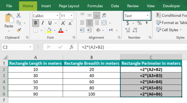
However, the target cells show the formulas instead of the formula values. The reason is that the target cells’ format is Text, as highlighted in the above image.
The solution is as follows:
• 1: First, select the target cells, C2:C6, and update the Number Format option in the Home tab as General.
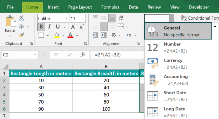
The “Number Format” is now in the “General” format.
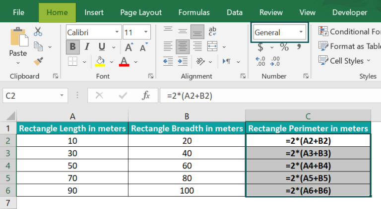
• 2: Double-click cell C2 to go to the edit mode.
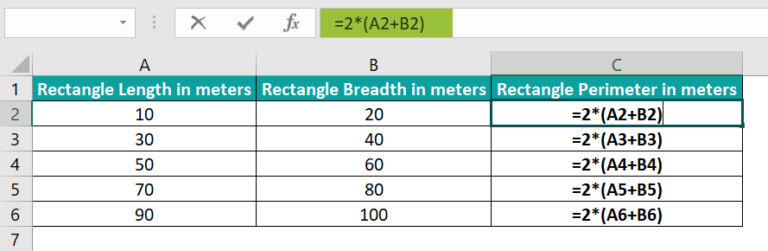
And press Enter.
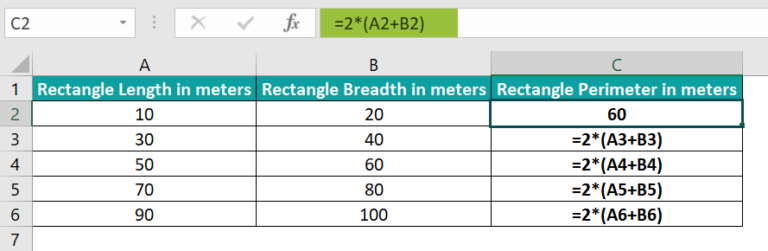
• 3: Drag the fill handle downwards to copy the formula in cells C3:C6.
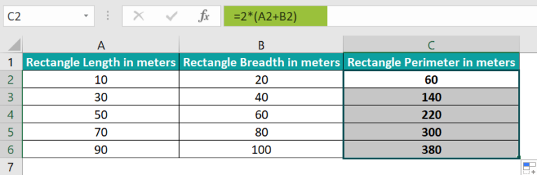
3. What happens when we enclose a worksheet name while referring to it in a formula in our active worksheet in double quotes?
When we enclose a worksheet name while referring to it in a formula in our active worksheet in double quotes, we will get the below error.
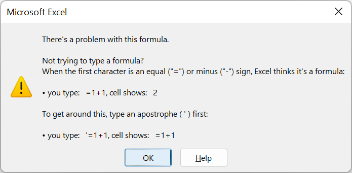
The solution to this issue is to remove the double quotations and enclose the worksheet name in single quotes if the name contains space. Otherwise, we can enter the worksheet name without quotes.
Download Template
This article must help understand the Excel formula not working, with its formula and examples. We can download the template here to use it instantly.
Recommended Articles
This has been a guide to Excel Formula Not Working. Here we see top 10 issues/errors we face in Excel, solutions, examples & a downloadable excel template. You can learn more from the following articles –
- Errors In Excel
- IFERROR in Excel
- ISERROR Excel Function
Microsoft Excel has been one of the most valuable tools since the dawn of modern computing. Over a million people use Microsoft Excel spreadsheets daily to manage projects, track finances, create charts and graphs, and even manage time.
Unlike other applications such as Word, the spreadsheet software uses mathematical formulas and data in cells to calculate values.
However, there are instances when the Excel formulas do not function properly. This article will help you fix problems with Excel formulas.
1. Calculation Options Set to Manual
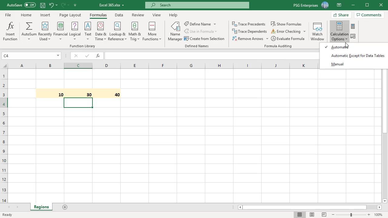
If you can’t update the value you’ve entered, and it returns the same as you entered, Excel’s calculation option may be set to manual and not automatic.
To fix this, change the calculation mode from Manual to Automatic.
- Open the spreadsheet you’re having trouble with.
- Then from the ribbon, navigate to the Formulas tab, then choose Calculation.
- Select Calculation Options and choose Automatic from the dropdown.
Alternatively, you can adjust the calculation options from Excel options.
Choose the Office button at the top left corner > Excel options > Formulas > Workbook Calculation > Automatic. If you often switch between these two modes, you can create a custom keyboard shortcut for Excel to speed up your work.
2. Cell Is Formatted as Text
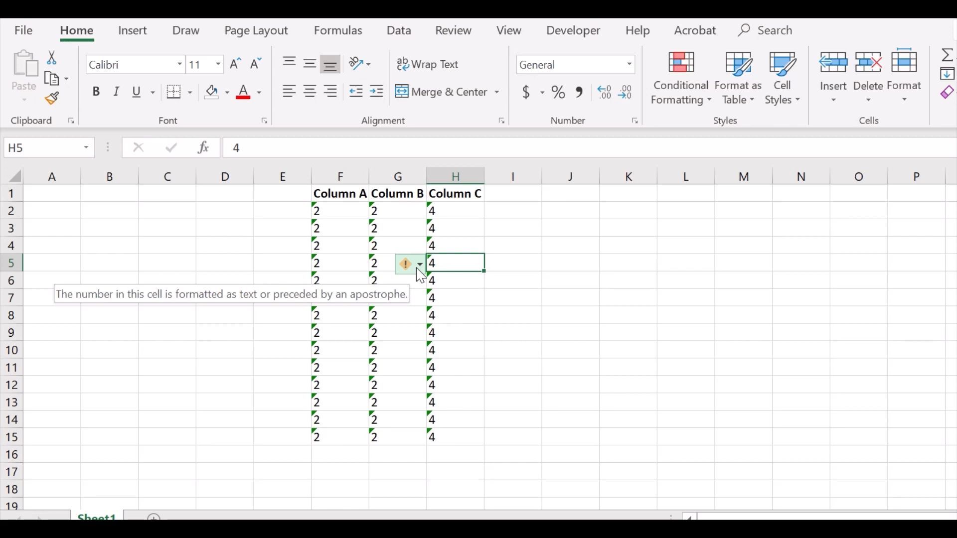
You might have accidentally formatted the cells containing the formulas as text. Unfortunately, Excel skips the applied formula when set to text format and displays the plain result instead.
The best way to check for formatting is to click on the cell and check the Number group from the Home tab. If it displays «Text,» click on that and choose General. To recalculate the formula, double-click the cell and press Enter on your keyboard.
3. Show Formulas Button Is Turned On
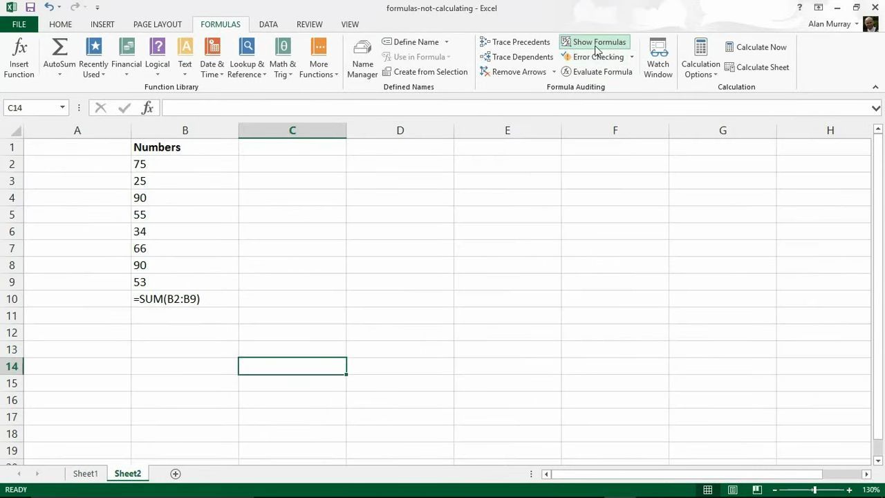
People commonly misuse the Show Formulas button by accidentally turning it on. With this turned on, the applied formulas will not work. You can find this setting under the Formulas tab.
The Show Formulas button is designed for auditing formulas, displaying the formula instead of the result when pressed. This might be a good tool if you want to better understand Excel formulas, but it stops them from working. In this case, turning it off may help resolve the issue.
Go to the Formulas tab > Formula Auditing Group and click the Show Formulas button.
4. Check Your Excel Formula

Even if you’re using an Excel function for beginners, a missing or an extra character might be why your Excel formula isn’t working. For example, when you enter an additional equal to (‘=’) or apostrophe (‘) in a spreadsheet cell, calculations are not performed, causing problems for users. The issue typically occurs when users try to copy a formula from the web.
However, it is simple to fix this problem. Just head over to the cell, select it, and remove the apostrophe or space at the beginning of the formula.
The same goes for the formula’s parentheses. When writing a lengthy formula, make sure you match all parentheses, so the calculations take place in the correct order. Excel helps you by showing parentheses pairs in different colors, so you can easily follow them.
Excel will display an error message when there’s a missing or extra parenthesis.
5. Use Proper Characters to Separate Arguments
You might have to separate function arguments to get the desired outcome depending on which Excel formulas you’re using. You should generally separate arguments using commas, but this may vary depending on your Regional Settings.
For example, in North American countries, you must enter commas to separate arguments, while in Europe, the right character is set to a semicolon. If you’ve used the wrong separating character, Excel might show the «We found a problem with this formula» error. You can try both options and check which one works for you.
If you’re used to using commas instead of semicolons, or vice versa, you can edit Excel settings to avoid repeating the same error.
- Open Excel’s File menu and go to More > Options.
- From the left pane, select Language.
- In the Office display language section, click the Add a language button.
- Select the wanted language to install and click Install.
- Select it again and click Set as Preferred.
- Test if Excel formulas are now working.
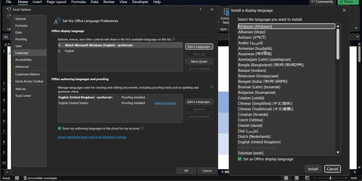
To sync Office settings across your devices when logging in with your Microsoft account, check the Store my authoring languages in the cloud for my account option.
6. Force Excel to Recalculate
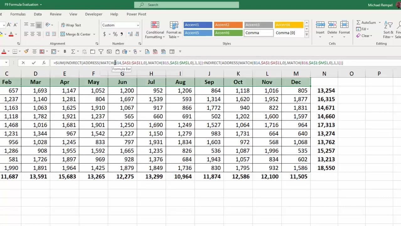
Excel allows users to recalculate formulas manually if they prefer not to use automatic calculation settings. You can do this with these methods:
For recalculating an entire spreadsheet, press F9 on your keyboard or choose Calculate Now under Formula Tab. Alternatively, you can recalculate an active sheet by pressing Shift + F9 on your keyboard or selecting Calculate Sheet from the Calculation group under Formula Tab.
You could also recalculate all formulas across all worksheets by pressing the Ctrl + Alt + F9 keyboard combination. Moreover, if you prefer recalculating just one formula from a sheet, select the cell and press Enter.
7. Check for Circular References
Excel formulas might show the wrong results if it uses circular referencing, which refers to the same cell where it does the calculations. Most of the time, Excel will notify you about a circular reference, but it might not do it every time.
Fortunately, you can manually check for this type of reference if you keep getting wrong results out of Excel formulas.
Open the Formulas tab, go to Formula Auditing, and select Error Checking > Circular References. Excel will show which cells have added a circular reference to the formula.
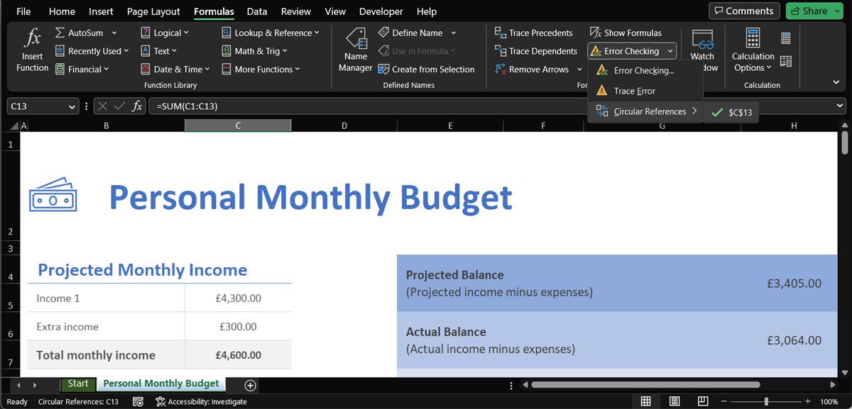
Go to the indicated cells and edit the formula so it doesn’t include the cell showing the results. For example, if the C13 cell shows the result for =SUM(C1:C13), change C13 to C12 within the formula to fix it.
Solve Your Excel Issues With These Fixes
The truth is, there’s not much room for error when writing an Excel formula. A missing parenthesis or the wrong cell format is enough to stop Excel formulas from working as intended.
However, you should know how to fix the issue as you’ll save a lot of time having Excel do the calculations for you.
Unable to make use of Excel formula because all of a sudden it stopped working, updating or calculating your data figures? Desperately you are looking for the fixes so that your Excel formula starts working again?
If your answer is yes then DON’T WORRY…! because you are at the right place.
This post will give you the best fixes to troubleshoot Excel Formulas Not Working, Excel formulas not updating or Excel formulas not calculating like issues.
I ensure you all that after reading the complete post you can proficiently fix Excel Formulas Not working issue on your own.
So, let’s dive into it….!
To recover Excel sheet data, we recommend this tool:
This software will prevent Excel workbook data such as BI data, financial reports & other analytical information from corruption and data loss. With this software you can rebuild corrupt Excel files and restore every single visual representation & dataset to its original, intact state in 3 easy steps:
- Download Excel File Repair Tool rated Excellent by Softpedia, Softonic & CNET.
- Select the corrupt Excel file (XLS, XLSX) & click Repair to initiate the repair process.
- Preview the repaired files and click Save File to save the files at desired location.
About Excel Formulas Error
Undoubtedly Excel provides a number of functions to analyze, audit, and calculate data. Some of these functions and formulas are frequently used by Excel users while some of them are specifically used by a small group of financial engineering or statistical specialist.
Excel file without a formula is impossible. Excel spreadsheet is all about formulas. Formulas make the work easy for maintaining and carrying out complex calculations as well. But what if you encounter Excel formulas not working issue? Well, it’s very frustrating as you are not able to do anything on your Excel file.
Let’s take an example for clear understanding:
Suppose you have created the reports for your management meeting and just before printing copies for the executives, you discover that totals are showing the last month values. This is very frustrating as you don’t know how to fix it?
When such instances occur several questions start running in mind that why my Excel formulas not calculating automatically? OR why don’t Excel formulas not updating automatically?
As it’s a very annoying situation so it’s obvious for any user to get Panic. But you need to be calm so that you can find out the actual reason for getting Excel formulas not working issue. To help you in this, my tutorial will explain the most common mistakes that you are doing while making formulas for Excel.
Types Of Excel Formula Errors:
Mostly it is seen that Excel users get stuck in three of these situations when their Excel formula starts troubling them.
- Excel formulas not working–
meanwhile this your Excel formula starts showing the wrong result or error.
- Excel formulas not updating–
It will display the old value even after you have already updated the dependent cells.
- Excel formulas not calculating–
In this case, the cell will only display the formula not give any result of it.
Here in this article, we are describing the complete information that explains the most common mistakes that happen while using a formula in Excel. So, that any Excel user can overcome Excel formula not calculating, Excel formula not updating automatically or Excel Formula not Working like issues easily and effortlessly.
How To Fix Excel Formulas Not Working Error?

The occurrence of Excel formula not working issue returns the wrong results or sometimes errors too. So, in this section, you will get an idea of how to fix silly mistakes usually done at the time of creating Excel formulas.
1. Enter Numbers Without Any Formatting
While using the Excel formula, don’t add a currency sign eg: $ or € or a decimal separator.
Note: in the Excel formulas, a sign of comma is generally used for separating the function of arguments. Whereas, the sign of dollar is for making absolute cell reference.
So, you can put a numeric value like this, 50000 instead of putting data like this $50,000. All in all, I just want to say in your Excel formula simply use the numeric value.
2. Numbers shouldn’t be formatted as text values
Another very common reason for the Excel formula not working is that numbers formatted as text values. It may look like as a normal number but MS Excel considers them as a text string and doesn’t include it in the calculations.

Visual indicators of a text editor are like this:
- Numbers that are formatted as “text” will by default get left-aligned while formal numbers are aligned right in the cells.
- You will see that on the Home tab> number group, the number format box is selected with Text option.
- When many cells having text numbers have been selected from the worksheet you will see that the Status Bar will only show the Count. whereas generally, it displays the count, sum, and average of numbers.
- You will see a green triangle shape in the cell’s top-left corner or a leading apostrophe visible in the formula bar.

To fix this, just select all the problems having cells and then tap on the yellow warning sign. After that select, the option Convert to Number.

But in some cases, nor the green triangles neither the warning signs seem in the cells. Then in that case go to the Home tab > Number group >number format box. if this shows the text, then clear all the formatting of the cells having the issue. after then set the format of the cell either general or number.
But if it still won’t work then make a new column and enter the data manually. Means just copy down your text to the notepad after then paste it on your Excel sheet. At the end delete off all broken columns.
3. Match All Opening And Closing Parentheses In A Formula

Generally, arguments of the Excel functions are kept under parentheses and in complex formulas; you may require to put more than a single set of the parentheses. When making such complex formula make sure that you have opened and closed the parenthesis properly.
Well, Excel shows parentheses pair in some different colors when you use it in the formula. Suppose your formula is lacking with some parentheses then Excel will display the error and allow you to correct it by balancing the pair. and due to this users start getting Excel Formulas Not Working error message.
4. Put All The Required Arguments Within The Excel Function

Each Excel function is having single or multiple required arguments. If you are entering optional arguments then enclosed it in the [square brackets] in your formula’s syntax. So, the formula must have all the necessary arguments. Or else your Excel will display the following “You’ve entered too few arguments for this function” warning message.
If the entered arguments are more than the required one then you will encounter with following “You’ve entered too many arguments for this function” warning message.
5. Include The Full Path To A Closed Workbook
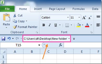
If you are using a formula that references a closed Excel workbook then your external reference must include the workbook name and entire path to the workbook. For example:
=SUM(‘D:Reports[Sales.xlsx]Jan’!B2:B10)
6. Don’t Nest More Than 64 Functions Within A Formula
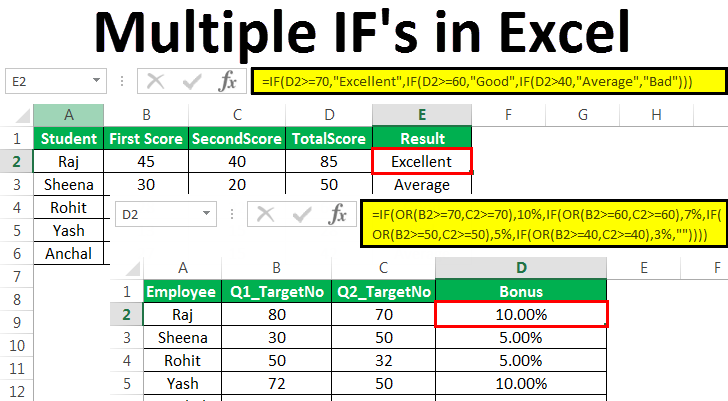
If you are nesting more than two Excel functions with each other for example suppose to create nested IF formula. Then follow these limitations:
- In Excel 2016/2013/2010/2007 you can make use of max 64 nested functions.
- While in Excel 2003 and lower, you can only make use of a maximum of 7 nested functions.
7. Don’t Enclose Numbers In Double Quotes

In the Excel formula; the value encoded within the double quotes counted as a text string.
That means, if you enter Excel formula like=IF(A1>0, “1”), then Excel will consider 1 as a text, and thus you won’t be able to make use of the returned 1’s in any other calculations. So, don’t put the double quotes and always write the formula for numeric value don’t enclose numbers in double-quotes until and unless you want it to count as text.
8. Enclose Workbook And Worksheet Names In Single Quotes
When referring to other worksheets or workbooks that have spaces or non-alphabetical characters in their names, enclose the names in single quotation marks.
For example Reference to another sheet:
=SUM(‘Jan Sales’!B2:B10)
Reference to another workbook:
=SUM(‘[2015 Sales.xlsx]Jan sales’!B2:B10)
9. Use Right Charcter For Separating The Function Argument
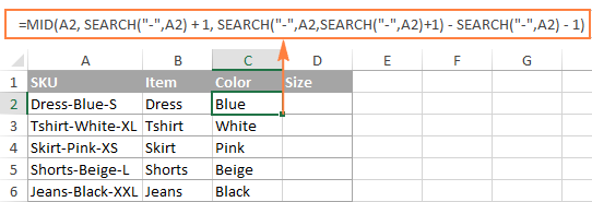
Most of you separate the Excel function arguments with the comma, however, this doesn’t work on all Excel workbook. The character which you generally use to divide arguments moreover depends on the List Separator which is sets with the Regional Settings.
European countries use for assigning the decimal symbol. Whereas, for the list separator semicolon; is used.
For e.g: North American excel user, would write =IF(A1>0, “OK”, “Not OK”), whereas European Excel users will put the exact same formula like this =IF(A1>0; “OK”; “Not OK”).
If you suddenly start getting Excel Formulas Not Working issue because of the “We found a problem with this formula…” error. in that case just go to your Regional Settings which is present in:
(Control Panel > Region and Language > Additional Settings)
After then make a check the character which is set for List Separator over there. make use of the same character for dividing the arguments in the formula of Excel.
Try the given tricks to solve the Microsoft Excel Formula not working and fix the error easily.
How To Fix Excel Formulas Not Updating Automatically?

When you are noticing that the Excel formula is not updating automatically the reason can be your Excel calculation setting is somehow got changed. Generally, it is found that when the calculation setting gets changed from automatic to manual. At that time Excel formula is not updating automatically like issues is been faced.
Here is how to change the calculation setting to fix Excel Formula Is Not Updating issue.
- Go to the Excel ribbon, and then on the Formulas.
- From this formula tab choose the Calculation group.
- tap to arrow key present next to Calculation Options. From the drop-down choose the Automatic option.

Or else, you can modify the calculation setting through these steps:
- For Excel 2019, Excel 2016, Excel 2013, and Excel 2010 user:
Open Excel worksheet < Formulas < Calculation options group. After then choose the Automatic option present within Workbook Calculation.
- For Excel 2007 user:
Tap to the Office button < Excel options < Formulas < Workbook Calculation < Automatic.

- For Excel 2003 user:
From your Excel ribbon choose the Tools < Options< Calculation< Calculation< Automatic.
How To Fix Excel Formulas Not Calculating Automatically?

If you are struggling with Excel Formulas Not Calculating issue then it’s because your cell is showing the Excel function in place of the evaluated value.
Behind this Excel formulas not calculating automatically error following are the reasons. So, check out the reasons along with its fixes to troubleshoot Excel formulas not calculating issues.
1. Show Formulas Mode Is Left On
One very common reason behind Excel formula not calculating error is that by mistakenly show formula mode has been activated in the worksheet.
So, to fix this Excel formula not calculating issue it’s compulsory to turn off Show Formulas mode.
Here is the step to be followed:
- Go to the Excel Formulas tab and from the Formula Auditing group tap to the Show Formulas

2. A Formula Is Entered As Text
The second reason behind the occurrence of Excel formula not calculating error is that Excel formulas is been formatted like text. For checking this out, follow these steps:
- From the Excel ribbon go to the home tab and then choose the Number group.
- Now choose the formula cell after then have a look over the Number Format box.
- If it’s showing text in the number group then change it to General and press F2 button from the keyword, being in the cell.
- Now enter any Excel formula so that it will recalculate the data again and show the calculated data.

Steps To Recalculate Excel data
If due to any reason, you want to set the Calculation option to Manual. In excel you have the option to force the Excel formulas to recalculate the data again. For this, you need to click on the calculate button.
So, check this out how to force the Excel formulas to recalculate:
For Recalculating Entire Workbook Data:
- From the Formulas tab choose the Calculation group.
- From the opened Calculation group tap to Calculate Now.
For Recalculating Any Specific Active Sheet:
- From the Formulas tab choose the Calculation group.
- From the opened Calculation group tap to Calculate Sheet.

If you to perform this recalculation task in all sheets of your opened Excel workbooks. Then for this just press the Ctrl + Alt + F9 button simultaneously.
In case you want to recalculate one single formula on the sheet then choose the formula cell. After then get into the editing mode by double-tapping the cell or by hitting the F2 button. At last hit Enter key from your keyboard.
Automatic Solution: MS Excel Repair Tool
Apart from the manual solution sometimes the Excel file gets corrupted and starts showing various errors, then, in this case, make use of the MS Excel Repair Tool. This is the best repair utility to fix all sorts of issues, corruption, and even errors in the Excel file.
With the help of these users can repair the Excel file easily and also restore the entire corrupted data including cell comments, charts, other data, and worksheet properties. This is a professionally designed program that can easily repair .xls and .xlsx files and easy to use.
* Free version of the product only previews recoverable data.
Steps to Utilize MS Excel Repair Tool:
Conclusion:
In this article, I tried my best to provide ample information to solve the Excel Formulas Not Working, calculating or updating error message. Make use of the given solution to fix the error and utilize the Excel file completely for maintaining crucial data.
Good Luck!!!


Priyanka is an entrepreneur & content marketing expert. She writes tech blogs and has expertise in MS Office, Excel, and other tech subjects. Her distinctive art of presenting tech information in the easy-to-understand language is very impressive. When not writing, she loves unplanned travels.