
Содержание
- What Do the Symbols (&,$,<, etc.) Mean in Formulas? – Excel & Google Sheets
- Equal Sign (=)
- Standard Operators
- Order of Operations and Adding Parentheses
- Colon (:) to Specify a Range of Cells
- Dollar Symbol ($) in an Absolute Reference
- Exclamation Point (!) to Indicate a Sheet Name
- Square Brackets [ ] to Refer to External Workbooks
- Comma (,)
- Refer to Multiple Ranges
- Separate Arguments in a Function
- Curly Brackets in Array Formulas
- Other Important Symbols
- Symbols in Formulas in Google Sheets
- Excel Symbols – what do they mean and how do I use them?
- Excel Symbols – do you know what they mean? Take a look at the list below!
- Excel Symbols List
- What Does $ (Dollar Symbol) Mean in Excel and How to Use It
- $ (Dollar Symbol) Meaning in Excel and Its Function
- How to Add a $ Symbol in an Excel Formula 1: Direct Typing
- How to Add a $ Symbol in an Excel Formula 2: The F4 Button (Command + T in Mac)
- Exercise
- Instructions
- Additional Note
What Do the Symbols (&,$,<, etc.) Mean in Formulas? – Excel & Google Sheets
This tutorial explains what different symbols mean in formulas in Excel and Google Sheets.
Excel is essentially used for keeping track of data and using calculations to manipulate this data. All calculations in Excel are done by means of formulas, and all formulas are made up of different symbols or operators, depending on what function the formula is performing.
Equal Sign (=)
The most commonly used symbol in Excel is the equal (=) sign. Every single formula or function used has to start with equals to let Excel know that a formula is being used. If you wish to reference a cell in a formula, it has to have an equal sign before the cell address. Otherwise, Excel just shows the cell address as standard text.
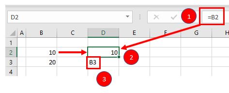
In the above example, if you type (1) =B2 in cell D2, it returns a value of (2) 10. However, typing only (3) B3 into cell D3 just shows “B3” in the cell, and there is no reference to the value 20.
Standard Operators
The next most common symbols in Excel are the standard operators as used on a calculator: plus (+), minus (–), multiply (*) and divide (/). Note that the multiplication sign is not the standard multiplication sign (x) but is depicted by an asterisk (*) while the division sign is not the standard division sign (÷) but is depicted by the forward slash (/).
An example of a formula using addition and multiplication is shown below:
Order of Operations and Adding Parentheses
In the formula shown above, B2*B3 is calculated first, as in standard mathematics. The order of operations is always multiplication before addition. However, you can adjust the order of operations by adding parentheses (round brackets) to the formula; any calculations between these parentheses would then be done first before the multiplication. Parentheses, therefore, are another example of symbols used in Excel.
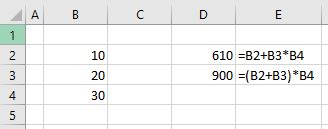
In the example shown above, the first formula returns a value of 610 while the second formula (using parentheses) returns 900.
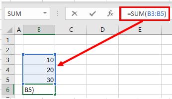
Parentheses are also used with all Excel functions. For example, to sum B3, B4, and B5 together, you can use the SUM Function where the range B3:B5 is contained within parentheses.
Colon (:) to Specify a Range of Cells
In the formula used above, the parentheses contain the cell range which the SUM Function needs to add together. This cell range is expressed with a colon (:) where the first cell reference (B3) is the cell address of the first cell included in the range of cells to add together, while the second cell reference (B5) is the cell address of the last cell included in the range.
Dollar Symbol ($) in an Absolute Reference
A particular useful and common symbol used in Excel is the dollar sign within a formula. Note that this does not indicate currency; rather, it’s used to “fix” a cell address in place in order that a single cell can be used repetitively in multiple formulas by copying formulas between cells.
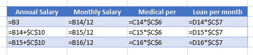
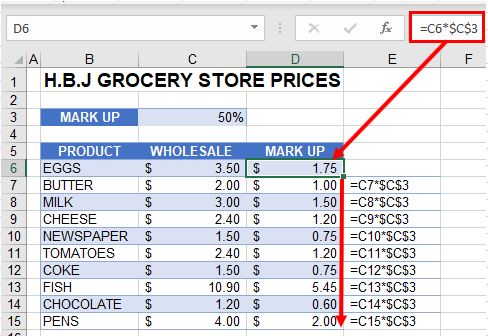
By adding a dollar sign ($) in front of the column header (C) and the row header (3), when copying the formula down to Rows 7–15 in the example below, the first part of the formula (e.g., C6) changes according to the row it is copied down to while the second part of the formula ($C$3) stays static always enabling the formula to refer to the value stored in cell C3.
See: Cell References and Absolute Cell Reference Shortcut for more information on absolute references.
Exclamation Point (!) to Indicate a Sheet Name
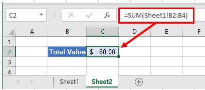
The exclamation point (!) is critical if you want to create a formula in a sheet and include a reference to a different sheet.
Square Brackets [ ] to Refer to External Workbooks
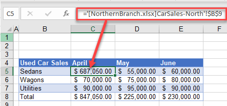
Excel uses square brackets to show references to linked workbooks. The name of the external workbook is enclosed in square brackets, while the sheet name in that workbook appears after the brackets with an exclamation point at the end.
Comma (,)
The comma has two uses in Excel.
Refer to Multiple Ranges
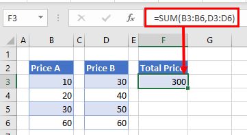
If you wish to use multiple ranges in a function (e.g., the SUM Function), you can use a comma to separate the ranges.
Separate Arguments in a Function
Alternatively, some built in Excel functions have multiple arguments which are usually separated with commas. (These can also be semicolons, depending on the function syntax.)
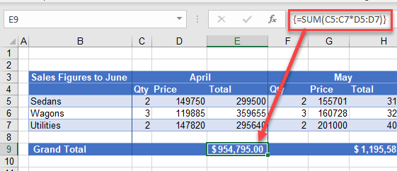
Curly Brackets in Array Formulas
Curly brackets are used in array formulas. An array formula is created by pressing the CTRL + SHIFT + ENTER keys together when entering a formula.
Other Important Symbols
| Symbol | Description | Example |
|---|---|---|
| % | Percentage | =B2% |
| ^ | Exponential operator | =B2^B3 |
| & | Concatenation | =B2&B3 |
| > | Greater than | =B2>B3 |
| = | Greater than or equal to | =B2>=B3 |
| Not equal to | =B2<>B3 |
Symbols in Formulas in Google Sheets
The symbols used in Google Sheets are identical to those used in Excel.
Источник
Excel Symbols – what do they mean and how do I use them?

Excel Symbols – do you know what they mean? Take a look at the list below!
This week’s blog is all about Excel symbols. They can be quite simple but if you don’t know what they mean it can be daunting or even frustrating! Some are a lot more obvious than others.
Excel is often used by a lot of people as a way of data entry and so people often do not have to use or understand what these symbols mean as they are already built into the spreadsheets that they use.
But have you ever been in a situation where you have clicked into a cell, exposed the formula and panicked at what you saw? All those symbols jumbled together and not knowing what they mean?
Don’t worry, it happens to us all! So because of this, we decided to put a table into our Basic course as a bit of a ‘Glossary’ to help when you start off learning about Excel! You can also find out a bit more about error messages in Excel by looking below at the list!
Excel Symbols List
Some of you would have been on our Basic Excel course and seen this list in your course notes you took away with you, however some of you wouldn’t have seen it.
So we thought we would share this list with you all that we put together of some of the common used basic symbols in Excel.
= This is an equal sign and is used at the beginning of a formula
+ This is an addition sign and is used in sums and formulas
– This is a subtraction sign and is used in sums and formulas
/ This is a division sign and is used in sums and formulas
* This is a multiplication sign and is used in sums and formulas
( ) These are rounded brackets and are used to group together smaller sums in more complex formulas
: This is a semi colon and is used in a formula to create a range of cells (e.g. A2:B4)
, This is a comma and is used for separating cell references in formulas (often for non-adjacent cells)
$ This is a dollar sign and is used when creating absolute references
% This is a percentage sign and is used when dealing with figures in percentages
[ ] These are square brackets and are used for identifying a workbook which is being linked into a formula
! This is an exclamation mark and is used for identifying a worksheet which is being linked into a formula
We hope you find this list useful! Let us know what you think!
These are all used in calculations and formulas in Excel and they are covered in more detail on our Basic and Intermediate Excel 1 day courses.
 Fed up of seeing error messages in your spreadsheets and not knowing what they mean?
Click here to find out more in our post on what different error messages in Excel mean.
If you want to have a look at what else is covered in our Excel courses, you can take a look at our agendas on our website here, also take a look at our customer comments section and see what others have thought when they have come on one of our courses!
Источник
What Does $ (Dollar Symbol) Mean in Excel and How to Use It


Got confused when you see $ symbols in an excel formula? Don’t know what they mean? This tutorial will answer what does $ mean in excel and how to use this symbol for you!
When we write a formula in excel, we often need to copy it to other cells. This is so we don’t have to waste time writing similar formulas again.
The $ symbol mainly helps us with this copy process so we get correct formula writings. Curious? Learn much more of the details below!
Disclaimer: This post may contain affiliate links from which we earn commission from qualifying purchases/actions at no additional cost for you. Learn more
Want to work faster and easier in Excel? Install and use Excel add-ins! Read this article to know the best Excel add-ins to use according to us!
$ (Dollar Symbol) Meaning in Excel and Its Function
The $ symbol in excel, more specifically in excel formulas, means that the row number/column letter on its right is absolute.
What does absolute mean? It means that the row number/column letter won’t move when we copy the formula to other cells!
You see, when we copy a formula in excel, the row and column in its cell references normally moves too. The movement depends on the direction where we copy the formula from the source.
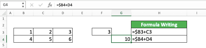
For example, take a look at the numbers and the manual sum formula in the screenshot below.
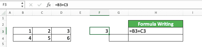
If we copy the sum formula to cell G4, then the result becomes like this.
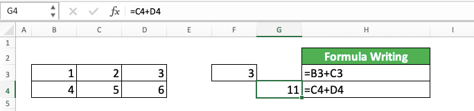
Why does the result become 11 not 3? That is because the cell references in the formula we copy also moves along with the copy direction.
As we copy the formula to one cell below and one cell right, its cell references also move in that direction. B3 becomes C4 (one cell below and one cell right from B3) and C3 becomes D4 (one cell below and one cell right from C3). This makes the sum formula sums 5 and 6 instead of 1 and 2, which produces 11.
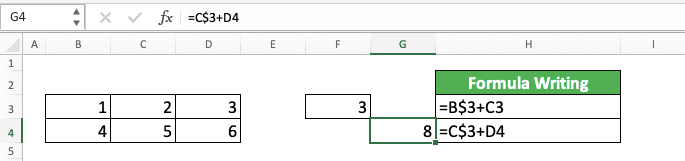
Now, what if we add a $ symbol in front of the B3 column letter before we copy the formula? That means the B3 writing in the formula becomes $B3 like this.

What will happen if we copy the formula to cell G4 like before? The thing that will happen is this.
Why the result now becomes 10 not 11? The reason is because we put a $ symbol in front of B in B3.
As discussed before, the $ symbol makes the row number/column letter on its right absolute. That means when we copy the formula with the $ symbol, the row/column won’t move.
In the example, the $ makes the B in B3 absolute. That makes the B letter won’t move when we copy the sum formula.
The formula result from the copy process is =$B4+D4. Only the row number in the $B3 moves and the column stays the same!
A similar thing will happen if we copy the formula with the $ symbol in front of the row number of B3. The row won’t move when we copy the formula because of that.
What if we put the $ symbol in front of both the row number and column letter of B3? That will make the cell reference won’t move both in its row and column when we copy the sum formula!

To summarize, here is a table that explains what a $ symbol does in an excel formula.
| $ Position | Meaning | Formula Writing Example |
|---|---|---|
| In front of the column letter | The column is an absolute reference (it won’t move wherever we copy the formula that contains the column reference) | =$A1 |
| In front of the row number | The row is an absolute reference (it won’t move wherever we copy the formula that contains the row reference) | =A$1 |
| In front of the row number and column letter | The column and row (the whole cell) are absolute references (they won’t move wherever we copy the formula that contains the cell coordinate reference) | =$A$1 |
Now, have you understood the meaning of the $ symbol in an excel formula? In short, it will make the row/column on its right won’t move when we copy the formula that contains it.
How to Add a $ Symbol in an Excel Formula 1: Direct Typing
As we have discussed the $ meaning in excel, now let’s talk about how to add it to your formula.
There are generally two methods to add $ symbols in excel, direct typing and using the F4 button. The following are the steps to add the $ symbol by typing it directly in your formula.
- Double click the cell where the formula you want to add the $ symbol is. Alternatively, highlight the formula cell and click on the formula bar

Type the $ symbols on the left of the row numbers/column letters you want to make absolute

How to Add a $ Symbol in an Excel Formula 2: The F4 Button (Command + T in Mac)
Another method to add $ symbols in your excel formula is by using the F4 button (Command + T in Mac). Here are the detailed steps to use the button for the purpose.
- Double click on the cell where the formula you want to add the $ symbol is. Alternatively, you can also highlight the formula cell and click on the formula bar

Place your typing cursor in the cell reference where you want to add the $ symbol by clicking it

Press the F4 (Command + T in Mac) button on your keyboard. Press it a few times if needed until the $ symbols are in the places you want in the cell
Exercise
After you learn about the $ meaning in excel and how to use it, you can do this exercise below. Doing it should help you understand how to use $ symbols in your excel formula.
Download the exercise file below and do the instructions. Download the answer key file if you have done the exercise and want to check your answer. Or probably when you are confused about how to do some of the instructions!
Link to the exercise file:
Download here
Instructions
Do each instruction in the appropriate sheet according to the instruction number (1=Sheet1, 2=Sheet2, 3=Sheet3)! Use $ symbols to help you answer them much faster!
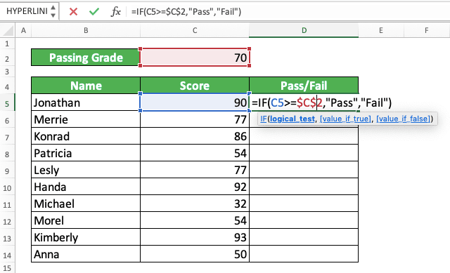
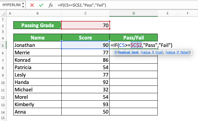
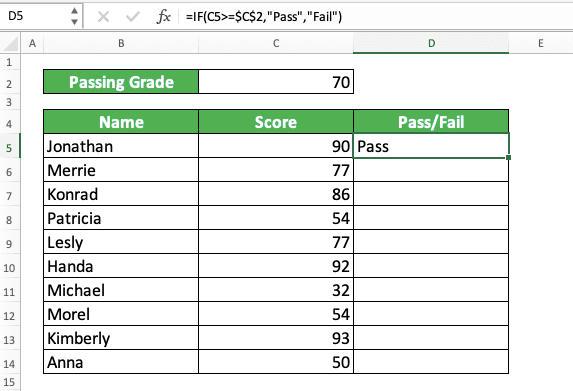
- Find out whether Mina, Klaus, and Lucia pass or fail on each of their subjects!
- Find out whether James, Patrick, and Nicole pass or fail on each of their subjects!
- Find the June, October, and March sales quantities from the table on the left using VLOOKUP!
Link to the answer key file:
Download here
Additional Note
If you want to add $ symbols in a cell range using F4, then do this. Highlight the cell range before you begin to press the button. You will automatically add $ symbols in both cells that represent the cell range!
Related tutorials you should learn:
Источник
This tutorial explains what different symbols mean in formulas in Excel and Google Sheets.
Excel is essentially used for keeping track of data and using calculations to manipulate this data. All calculations in Excel are done by means of formulas, and all formulas are made up of different symbols or operators, depending on what function the formula is performing.
Equal Sign (=)
The most commonly used symbol in Excel is the equal (=) sign. Every single formula or function used has to start with equals to let Excel know that a formula is being used. If you wish to reference a cell in a formula, it has to have an equal sign before the cell address. Otherwise, Excel just shows the cell address as standard text.
In the above example, if you type (1) =B2 in cell D2, it returns a value of (2) 10. However, typing only (3) B3 into cell D3 just shows “B3” in the cell, and there is no reference to the value 20.
Standard Operators
The next most common symbols in Excel are the standard operators as used on a calculator: plus (+), minus (–), multiply (*) and divide (/). Note that the multiplication sign is not the standard multiplication sign (x) but is depicted by an asterisk (*) while the division sign is not the standard division sign (÷) but is depicted by the forward slash (/).
An example of a formula using addition and multiplication is shown below:
=B1+B2*B3Order of Operations and Adding Parentheses
In the formula shown above, B2*B3 is calculated first, as in standard mathematics. The order of operations is always multiplication before addition. However, you can adjust the order of operations by adding parentheses (round brackets) to the formula; any calculations between these parentheses would then be done first before the multiplication. Parentheses, therefore, are another example of symbols used in Excel.
=(B1+B2)*B3
In the example shown above, the first formula returns a value of 610 while the second formula (using parentheses) returns 900.
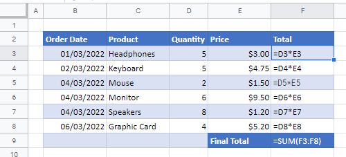
Parentheses are also used with all Excel functions. For example, to sum B3, B4, and B5 together, you can use the SUM Function where the range B3:B5 is contained within parentheses.
=SUM(B3:B5)Colon (:) to Specify a Range of Cells
In the formula used above, the parentheses contain the cell range which the SUM Function needs to add together. This cell range is expressed with a colon (:) where the first cell reference (B3) is the cell address of the first cell included in the range of cells to add together, while the second cell reference (B5) is the cell address of the last cell included in the range.
Dollar Symbol ($) in an Absolute Reference
A particular useful and common symbol used in Excel is the dollar sign within a formula. Note that this does not indicate currency; rather, it’s used to “fix” a cell address in place in order that a single cell can be used repetitively in multiple formulas by copying formulas between cells.
=C6*$C$3By adding a dollar sign ($) in front of the column header (C) and the row header (3), when copying the formula down to Rows 7–15 in the example below, the first part of the formula (e.g., C6) changes according to the row it is copied down to while the second part of the formula ($C$3) stays static always enabling the formula to refer to the value stored in cell C3.
See: Cell References and Absolute Cell Reference Shortcut for more information on absolute references.
Exclamation Point (!) to Indicate a Sheet Name
The exclamation point (!) is critical if you want to create a formula in a sheet and include a reference to a different sheet.
=SUM(Sheet1!B2:B4)
Square Brackets [ ] to Refer to External Workbooks
Excel uses square brackets to show references to linked workbooks. The name of the external workbook is enclosed in square brackets, while the sheet name in that workbook appears after the brackets with an exclamation point at the end.
Comma (,)
The comma has two uses in Excel.
Refer to Multiple Ranges
If you wish to use multiple ranges in a function (e.g., the SUM Function), you can use a comma to separate the ranges.
=SUM(B2:B3, B6:B10)
Separate Arguments in a Function
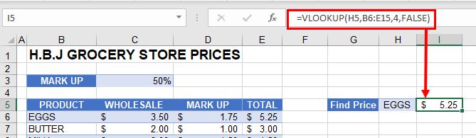
Alternatively, some built in Excel functions have multiple arguments which are usually separated with commas. (These can also be semicolons, depending on the function syntax.)
=VLOOKUP(H5, B6:E15, 4, FALSE)
Curly Brackets { } in Array Formulas
Curly brackets are used in array formulas. An array formula is created by pressing the CTRL + SHIFT + ENTER keys together when entering a formula.
Other Important Symbols
| Symbol | Description | Example |
|---|---|---|
| % | Percentage | =B2% |
| ^ | Exponential operator | =B2^B3 |
| & | Concatenation | =B2&B3 |
| > | Greater than | =B2>B3 |
| < | Less than | =B2<B3 |
| >= | Greater than or equal to | =B2>=B3 |
| <= | Less than or equal to | =B2<=B3 |
| <> | Not equal to | =B2<>B3 |
Symbols in Formulas in Google Sheets
The symbols used in Google Sheets are identical to those used in Excel.
Excel Symbols – do you know what they mean? Take a look at the list below!
![]() This week’s blog is all about Excel symbols. They can be quite simple but if you don’t know what they mean it can be daunting or even frustrating! Some are a lot more obvious than others.
This week’s blog is all about Excel symbols. They can be quite simple but if you don’t know what they mean it can be daunting or even frustrating! Some are a lot more obvious than others.
Excel is often used by a lot of people as a way of data entry and so people often do not have to use or understand what these symbols mean as they are already built into the spreadsheets that they use.
But have you ever been in a situation where you have clicked into a cell, exposed the formula and panicked at what you saw? All those symbols jumbled together and not knowing what they mean?
Don’t worry, it happens to us all! So because of this, we decided to put a table into our Basic course as a bit of a ‘Glossary’ to help when you start off learning about Excel! You can also find out a bit more about error messages in Excel by looking below at the list!
Excel Symbols List
Some of you would have been on our Basic Excel course and seen this list in your course notes you took away with you, however some of you wouldn’t have seen it.
So we thought we would share this list with you all that we put together of some of the common used basic symbols in Excel.
= This is an equal sign and is used at the beginning of a formula
+ This is an addition sign and is used in sums and formulas
– This is a subtraction sign and is used in sums and formulas
/ This is a division sign and is used in sums and formulas
* This is a multiplication sign and is used in sums and formulas
( ) These are rounded brackets and are used to group together smaller sums in more complex formulas
: This is a semi colon and is used in a formula to create a range of cells (e.g. A2:B4)
, This is a comma and is used for separating cell references in formulas (often for non-adjacent cells)
$ This is a dollar sign and is used when creating absolute references
% This is a percentage sign and is used when dealing with figures in percentages
[ ] These are square brackets and are used for identifying a workbook which is being linked into a formula
! This is an exclamation mark and is used for identifying a worksheet which is being linked into a formula
We hope you find this list useful! Let us know what you think!
These are all used in calculations and formulas in Excel and they are covered in more detail on our Basic and Intermediate Excel 1 day courses.
Fed up of seeing error messages in your spreadsheets and not knowing what they mean?
Click here to find out more in our post on what different error messages in Excel mean.
If you want to have a look at what else is covered in our Excel courses, you can take a look at our agendas on our website here, also take a look at our customer comments section and see what others have thought when they have come on one of our courses!
If you have worked with Excel formulas, I am sure you have noticed that sometimes there is a $ symbol as a part of the cell references.
If you’re wondering what does the $ sign means in Excel formulas/functions, this article is the right place.
One of the things that make Excel such a powerful tool is the ability to refer to cells/ranges and use these in formulas.
And when you copy these formulas, these cell references can adjust automatically (or should I say automatically).
Below is an example where I copy the cell C2 (which has a formula) and paste it in C3.
You can see that the formula adjusts the references when I copy and paste it. While in the formula in cell C2 refers to A2 and B2, the one in C3 refers to A3 and B3.
This is called relative reference where the references adjust based on the cell in which it has been applied.
But what if you don’t want some cells to adjust the reference?
What if you want to copy the formula, but don’t want the cell reference to change?
…. introducing the $ sign.
When you use a $ sign before the cell reference (such as $C$2), you’re telling Excel to keep referring to cell C3 even when you copy and paste the formula.
Now you can use the dollar ($) sign in three different ways, which means that there are three types of references on Excel.
Shortcut to add $ Sign to Cell References
There are two ways you can add the $ sign to a cell reference in Excel.
You can either do it manually (i.e., go into the edit mode in a cell by double-clicking on it or using F2, placing the cursor where you want the $ sign and then typing it manually).
Or you can use the keyboard shortcut
F4
To use this shortcut, simply place the cursor on the cell reference where you want to add the dollar sign and press is once. You will notice that it will change the reference by adding/removing the $ sign (based on what’s the original reference).
For example, suppose you have the reference C2 in a cell. Here is how the F4 shortcut would work:
- Press F4 one time – C2 will change to $C$2
- Press F4 two times – C2 will change to C$2
- Press F4 three times – C2 will change to $C2
- Press F4 four times – C2 will change back to C2
Types of References in Excel
There are three types of references in Excel:
- Relative references
- Absolute references
- Mixed references
In relative references, you don’t use a dollar ($) sign in the references at all.
In mixed references, you use the dollar sign ($) only once (such as $C3 or C$3)
In absolute reference, you use the dollar sign in twice in a reference (such as $C$3).
Let me quickly explain each of these with a simple example.
Relative reference
Relative reference is where you don’t use a dollar ($) sign at all.
And when you copy a cell that has a relative reference, it will change and adjust based on the cell where you copy it.
Below is the same example again, where the references adjust as soon as we copy and paste the cell that has the formula.
Absolute reference
In absolute references, you have the $ sign before the row number and the column alphabet (example $C$3)
When you use this in formulas, it will not change the reference
when you copy and paste the cell. This could be useful when you have some value that needs to remain constant (such as time period or interest rates, etc.)
Below is an example where I have a value in cell D2 which needs to remain constant (and not change when we copy-paste the formulas).
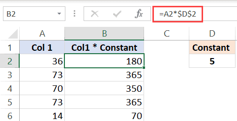
By using $D$2, we make sure that it doesn’t change when we copy-paste the cell with the formula.
Note that this example has both, relative cell reference (without the $ sign) and an absolute cell reference (with two $ signs).
Note: If you’re wondering why not simply hard code the value instead of using the absolute cell reference (the one with two dollar signs). While you can use the value itself, in the future, if you have to change the value in formulas, you will have to manually do it. Instead, you can simply change the value in C3, and all the formulas would automatically update.
Mixed reference
These are a little more complicated than the rest two.
In mixed cell references, you will have only one dollar sign (for example – $C3 or C$3)
When you add a dollar sign in front of the column alphabet (C in this example), it locks the column only. This means that if you copy-paste the formula that uses $C3, the column would not change, but the row can change.
And when you add a dollar sign in front of the row number (3 in this example), it locks the column only. This means that if you copy-paste the formula that uses C$3, the row would not change, but the column can change.
Here is a good article that goes in-depth about the mixed cell references in Excel.
Summary
A dollar sign means that the part of the cell reference before which it has been used is anchored or fixed.
Below is a quick summary of what $ means in Excel formulas:
- $A$1 – always refers to column A and row 1
- $A1 – Column A is fixed and will not change, but the row is allowed to change as the formula is copied
- A$1 – Row 1 is fixed and will not change, but the column is allowed to change as the formula is copied.
- $A$1:$A$100 – always refers to the range A1:A100
I hope this article helps you understand what the $ sign means in Excel and how to use it.
Other Excel tutorials you may find useful:
- How to Remove Dollar Sign in Excel
- How to Remove Dashes (-) in Excel?
- How to Lock Cells in Excel [Mac, Windows]
- How to Apply Accounting Number Format in Excel
- What does Pound/Hash Symbol (####) Mean in Excel?
- What Does the Exclamation Point Mean in Excel?
There are many functions in order to find the average in Excel (although it does not matter what kind of value it is: numerical, textual, percentage or other). And each of them has its own peculiarities and advantages. After all, certain conditions can be put in this task.
For example, the average in Excel is counting using statistical functions. You can also manually enter your own formula. Consider the various options.
How to find the arithmetic mean?
It is necessary to add all the numbers in the set and divide the sum by the number in order to find the arithmetic mean. For example, the student’s marks in computer science: 3, 4, 3, 5, 5. The average rating is 4 for a quarter. We found the arithmetic mean using the formula: =(3 + 4 + 3 + 5 + 5) / 5.
How can you quickly do this with Excel functions? Take for example a number of random numbers in a row:

- We put the cursor in cell A2 (under a set of numbers). In the menu – «HOME»-«Editing»-«AutoSum»-«Average» button. A formula appears after clicking in the active cell. Select the range: A1: H1 and press ENTER.
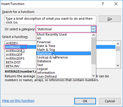
- The second method is based on the same principle of finding the arithmetic mean. But we will call the function AVERAGE differently. Using the function wizard (use fx button or key combination SHIFT + F3).
- The third way to call the AVERAGE function from the panel: «FORMULAS»-«More Function»-«Statistical»-«AVERAGE».
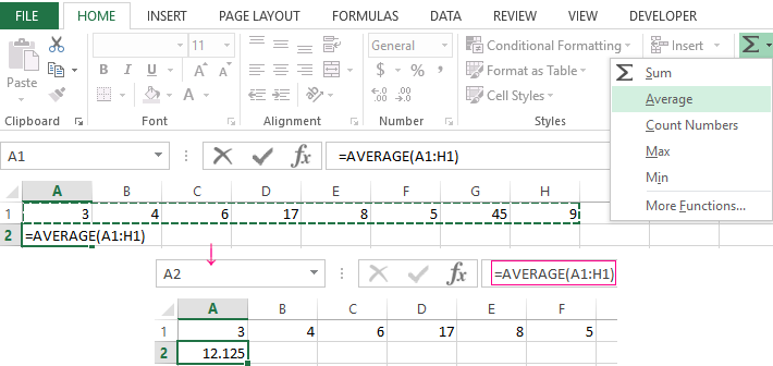
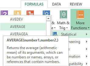
Or you can make cell to be active and just manually enter the formula: =AVERAGE(A1:A8).
Now let’s see what the AVERAGE function be able to:
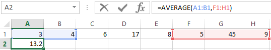
Let us find the arithmetic mean of the first two and three last numbers. Formula: =AVERAGE(A1:B1,F1:H1).
Average value by condition
A numerical criterion or a textual criterion can be the condition for finding the arithmetic mean. We will use the function: = AVERAGEIF().
Find the arithmetic mean for numbers that are greater or equal to 10.
Function:
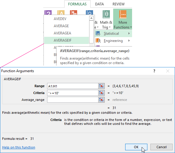
The result of using the function «AVERAGEIF» by the condition «>=10» is next:
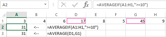
The third argument «Averaging Range» is omitted. Firstly, it is not necessary. Secondly, the range analyzed by the program contains ONLY numeric values. In the cells specified in the first argument, the search will be performed according to the condition specified in the second argument.
Attention! You can specify the search criteria in the cell. And in the formula make a reference to it.
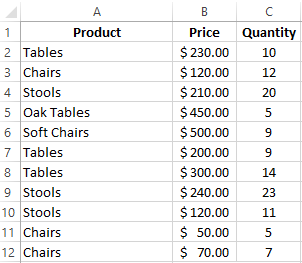
Let’s find the average value of numbers by the text criterion. For example, the average sales of goods «Tables».
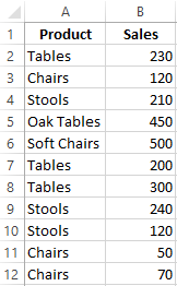
The function will look like this:
Range is a column with the names of goods. Search criteria is a link to a cell with the word «Tables» (you can insert the word «Tables» instead of the A7 link). The averaging range is the cells from which data will be taken to calculate the arithmetic mean.
We get the following value as a result of calculating using the function:
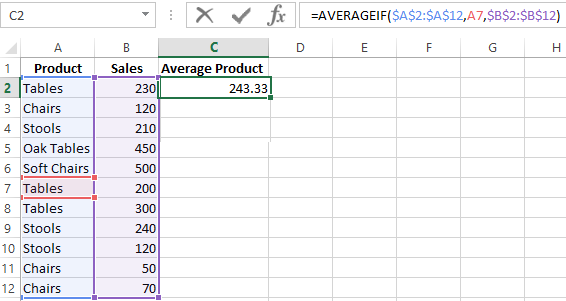
Attention! It is mandatory to point the averaging range for the text criterion (condition).
How to calculate the weighted average price in Excel?
How to calculate the average percentage in Excel? For this purpose, the SUMPRODUCTS and SUM functions are suitable. Table for an example:
How did we know the weighted average price?
Formula:
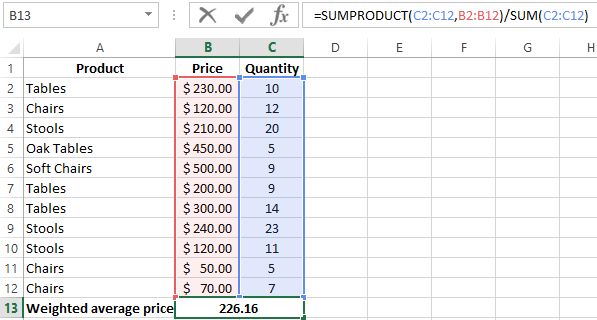
Using the formula =SUMPRODUCT() we learn the total revenue after the realization of the entire quantity of goods. And the =SUM() function sums the goods quantity. We found a weighted average price having divided the total revenue from the sale of goods by the total number of units of the goods. This indicator takes into account the «weight» of each price and its share in the total mass of values.
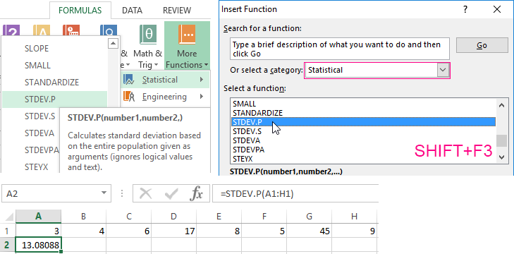
The standard deviation: the formula in Excel
There is a standard deviation in the entire population and in the sampling. In the first case, this is the square root of the general variance. In the second, this is a square root of the sampling variance.
A dispersion formula is compiled to calculate this statistical indicator. The square root is extracted from it. But in Excel, there is a ready-made function for finding the root-mean-square deviation.
The root-mean-square deviation is related to the scope of the initial data. This is not enough for a figurative representation of the variation of the analyzed range. The coefficient of variation is calculated to obtain the relative level of the data variability.
standard deviation / arithmetic mean
The formula in Excel is as follows:
STDEV.P (range of values) / AVERAGE (range of values).
The coefficient of variation is considered as a percentage. Therefore, set the percentage format in the cell set.
How to Find Mean in Excel (Table of Content)
- Introduction to Mean in Excel
- Example of Mean in Excel
Introduction to Mean in Excel
The average function is used to calculate the Arithmetic Mean of the given input. It is used to do sum of all arguments and divide it by the count of arguments where the half set of the number will be smaller than the mean, and the remaining set will be greater than the mean. It will return the arithmetic mean of the number based on provided input. It is an in-built Statistical function. A user can give 255 input arguments in the function.
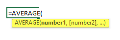
As an example, suppose there is 4 number 5,10,15,20 if a user wants to calculate the mean of the numbers then it will return 12.5 as the result of =AVERAGE (5, 10, 15, 20).
The formula of Mean: It is used to return the mean of the provided number where a half set of the number will be smaller than the number, and the remaining set will be greater than the mean.
The argument of the Function:
- number1: It is a mandatory argument in which functions will take to calculate the mean.
- [number2]: It is an optional argument in the function.
Examples on How to Find Mean in Excel
Here are some examples of how to find mean in excel with the steps and the calculation
You can download this How to Find Mean Excel Template here – How to Find Mean Excel Template
Example #1 – How to Calculate the Basic Mean in Excel
Let’s assume there is a user who wants to perform the calculation for all numbers in Excel. Let’s see how we can do this with the average function.
Step 1: Open MS Excel from the start menu >> Go to Sheet1, where the user has kept the data.
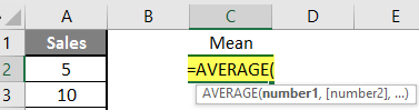
Step 2: Now create headers for Mean where we will calculate the mean of the numbers.
![]()
Step 3: Now calculate the mean of the given number by average function>> use the equal sign to calculate >> Write in cell C2 and use average>> “=AVERAGE (“
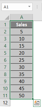
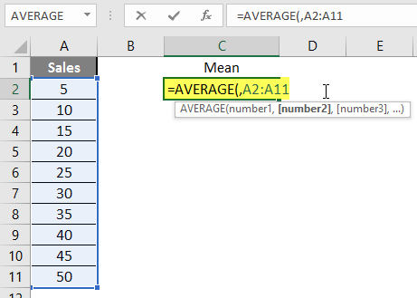
Step 3: Now, it will ask for a number1, which is given in column A >> there are 2 methods to provide input either a user can give one by one or just give the range of data >> select data set from A2 to A11 >> write in cell C2 and use average>> “=AVERAGE (A2: A11) “
Step 4: Now press the enter key >> Mean will be calculated.
Summary of Example 1: As the user wants to perform the mean calculation for all numbers in MS Excel. Easley everything calculated in the above excel example, and the Mean is 27.5 for sales.
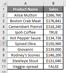
Example #2 – How to Calculate Mean if Text Value Exists in the Data Set
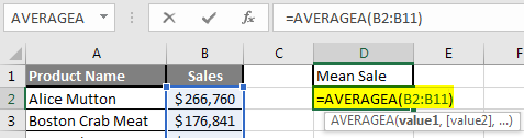
Let’s calculate the Mean if there is some text value in the Excel data set. Let’s assume a user wants to perform the calculation for some sales data set in Excel. But there is some text value also there. So, he wants to use count for all, either its text or number. Let’s see how we can do this with the AVERAGE function. Because in the normal AVERAGE function, it will exclude the text value count.
Step 1: Open MS Excel from the start menu >> Go to Sheet2, where the user has kept the data.
Step 2: Now create headers for Mean where we will calculate the mean of the numbers.
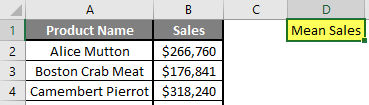
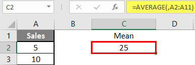
Step 3: Now calculate the mean of the given number by average function>> use the equal sign to calculate >> Write in cell D2 and use AVERAGEA>> “=AVERAGEA (“
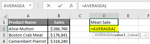
Step 4: Now, it will ask for a number1, which is given in column B >> there is two open to provide input either a user can give one by one or just give the range of data >> select data set from B2 to B11 >> write in D2 Cell and use average>> “=AVERAGEA (D2: D11) “
Step 5: Now click on the enter button >> Mean will be calculated.
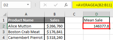
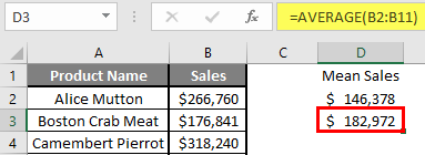
Step 6: Just to compare the AVERAGEA and AVERAGE, in normal average, it will exclude the count for text value so mean will high than the AVERAGE MEAN.
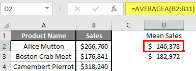
Summary of Example 2: As the user wants to perform the mean calculation for all number in MS Excel. Easley, everything calculated in the above excel example and the Mean is $146377.80 for sales.
Example #3 – How to Calculate Mean for Different Set of Data
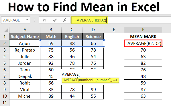
Let’s assume a user wants to perform the calculation for some student’s mark data set in MS Excel. There are ten student marks for Math, English, and Science out of 100. Let’s see How to Find Mean in Excel with the AVERAGE function.
Step 1: Open the MS Excel from the start menu >> Go to Sheet3, where the user kept the data.
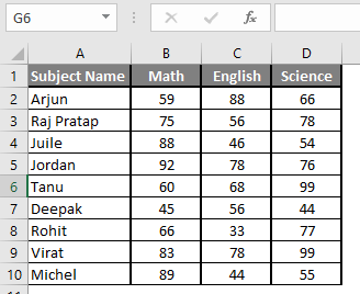
Step 2: Now create headers for Mean where we will calculate the mean of the numbers.
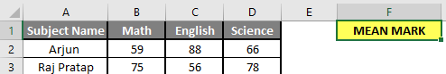
Step 3: Now calculate the mean of the given number by average function>> use the equal sign to calculate >> Write in F2 Cell and use AVERAGE >> “=AVERAGE (“
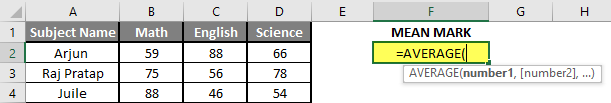
Step 3: Now, it will ask for number1 which is given in B, C, and D column >> there is two open to provide input either a user can give one by one or just give the range of data >> Select data set from B2 to D2 >> Write in F2 Cell and use average >> “=AVERAGE (B2: D2) “
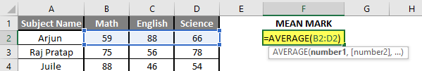
Step 4: Now click on the enter button >> Mean will be calculated.
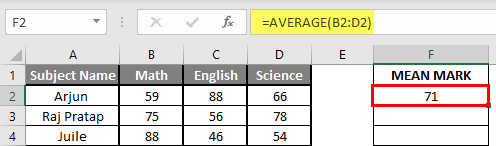
Step 5: Now click on the F2 cell and drag and apply to another cell in the F column.
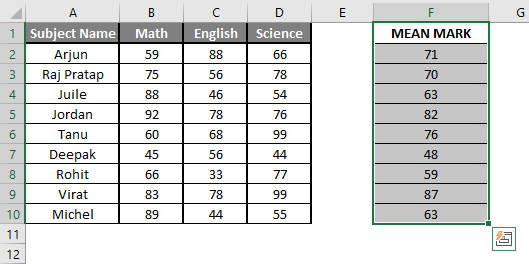
Summary of Example 3: As the user wants to perform the mean calculation for all number in MS Excel. Easley, everything calculated in the above excel example and the Mean is available in the F column.
Things to Remember About How to Find Mean in Excel
- Microsoft Excel’s AVERAGE function used to calculate the Arithmetic Mean of the given input. A user can give 255 input arguments in the function.
- Half the set of a number will be smaller than the mean, and the remaining set will be greater than the mean.
- If a user calculating the normal average, it will exclude the count for a text value, so AVERAGE Mean will bigger than the AVERAGE MEAN.
- Arguments can be number, name, range or cell references that should contain a number.
- If a user wants to calculate the mean with some condition, then use AVERAGEIF or AVERAGEIFS.
Recommended Articles
This is a guide to How to Find Mean in Excel. Here we discuss How to Find Mean along with examples and a downloadable excel template. You may also look at the following articles to learn more –
- FIND Function in Excel
- Excel Find
- Excel Average Formula
- Excel AVERAGE Function
![]()
Symbols Used in Excel Formula

Here are the important symbols used in Excel Formulas. Each of these special characters have used for different purpose in Excel. Let us see complete list of symbols used in Excel Formulas, its meaning and uses.
Symbols used in Excel Formula
Following symbols are used in Excel Formula. They will perform different actions in Excel Formulas and Functions.
| Symbol | Name | Description |
|---|---|---|
| = | Equal to | Every Excel Formula begins with Equal to symbol (=).
Example:=A1+A5 |
| () | Parentheses | All Arguments of the Excel Functions specified between the Parentheses.
Example:=COUNTIF(A1:A5,5) |
| () | Parentheses | Expressions specified in the Parentheses will be evaluated first. Parentheses changes the order of the evaluation in Excel Formula.
Example: =25+(35*2)+5 |
| * | Asterisk | Wild card operator to to denote all values in a List.
Example: =COUNTIF(A1:A5,”*“) |
| , | Comma | List of the Arguments of a Function Separated by Comma in Excel Formula.
Example: =COUNTIF(A1:A5,“>” &B1) |
| & | Ampersand | Concatenate Operator to connect two strings into one in Excel Formula.
Example: =”Total: “&SUM(B2:B25) |
| $ | Dollar | Makes Cell Reference as Absolute in Excel Formula.
Example:=SUM($B$2:$B$25) |
| ! | Exclamation | Sheet Names and Table Names Followed by ! Symbol in Excel Formula.
Example: =SUM(Sheet2!B2:B25) |
| [] | Square Brackets | Uses to refer the Field Name of the Table (List Object) in Excel Formula.
Example:=SUM(Table1[Column1]) |
| {} | Curly Brackets | Denote the Array formula in Excel.
Example: {=MAX(A1:A5-G1:G5)} |
| : | Colon | Creates references to all cells between two references.
Example: =SUM(B2:B25) |
| , | Comma | Union Operator will combine the multiple references into One.
Example: =SUM(A2:A25, B2:B25) |
| (space) | Space | Intersection Operator will create common reference of two references.
Example: =SUM(A2:A10 A5:A25) |
Share This Story, Choose Your Platform!
6 Comments
-
Redjen
May 31, 2022 at 12:37 pm — Replywhat is the symbol of average in excel?
-
PNRao
June 20, 2022 at 12:40 pm — ReplyYou can use AVERAGE()Function to calculate Average in Excel. If you wants to show the Average Statistical Symbol (x-bar), You can insert from symbols. F7C2 is the Unicode Hexa character for X-bar symbol. Make sure that you have set the Symbol Font :MS Reference Sans Serif.
-
-
Tom Pearce
September 22, 2022 at 3:54 pm — ReplyI have a workbook, where the original author used an @ sign in front of a function call in a formula. I can find no reference as to what the @ does, or how it is used. Any one know??
VBA Example: ActiveSheet.Range(“L2”).Formula = “=@CATEGORY($E2,LFC_AreaLU)”
Note: Category is a User Defined Function in the workbook.-
PNRao
December 5, 2022 at 11:30 am — Reply
-
-
Jane Girard
February 9, 2023 at 8:53 pm — ReplyI have this formula, do you know what the al means in the formula ?
IF(E4=””,””,VLOOKUP(C4,al,5,0)*E4), can-
PNRao
February 27, 2023 at 3:10 am — ReplyIt could be a defined Name or a name of the Table (List Object)
-
© Copyright 2012 – 2020 | Excelx.com | All Rights Reserved
Page load link
Google doesn’t understand <> so that failed thus asking here.
What does ‘<>’ (less than followed by greater than) mean in Excel? For example:
=SUMPRODUCT((E37:N37>0)*(E37:N37<>"")*(E37:N37))
What’s happening here?
![]()
Joey Adams
41.5k18 gold badges85 silver badges115 bronze badges
asked Jul 9, 2011 at 13:45
![]()
0
It means «not equal to» (as in, the values in cells E37-N37 are not equal to "", or in other words, they are not empty.)
answered Jul 9, 2011 at 13:47
![]()
James AllardiceJames Allardice
164k21 gold badges332 silver badges311 bronze badges