
Excel for Microsoft 365 Excel for Microsoft 365 for Mac Excel for the web Excel 2021 Excel 2021 for Mac Excel 2019 Excel 2019 for Mac Excel 2016 Excel 2016 for Mac Excel 2013 Excel 2010 Excel 2007 Excel for Mac 2011 Excel Starter 2010 More…Less
The SUMPRODUCT function returns the sum of the products of corresponding ranges or arrays. The default operation is multiplication, but addition, subtraction, and division are also possible.
In this example, we’ll use SUMPRODUCT to return the total sales for a given item and size:
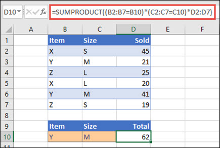
SUMPRODUCT matches all instances of Item Y/Size M and sums them, so for this example 21 plus 41 equals 62.
Syntax
To use the default operation (multiplication):
=SUMPRODUCT(array1, [array2], [array3], …)
The SUMPRODUCT function syntax has the following arguments:
|
Argument |
Description |
|---|---|
|
array1 Required |
The first array argument whose components you want to multiply and then add. |
|
[array2], [array3],… Optional |
Array arguments 2 to 255 whose components you want to multiply and then add. |
To perform other arithmetic operations
Use SUMPRODUCT as usual, but replace the commas separating the array arguments with the arithmetic operators you want (*, /, +, -). After all the operations are performed, the results are summed as usual.
Note: If you use arithmetic operators, consider enclosing your array arguments in parentheses, and using parentheses to group the array arguments to control the order of arithmetic operations.
Remarks
-
The array arguments must have the same dimensions. If they do not, SUMPRODUCT returns the #VALUE! error value. For example, =SUMPRODUCT(C2:C10,D2:D5) will return an error since the ranges aren’t the same size.
-
SUMPRODUCT treats non-numeric array entries as if they were zeros.
-
For best performance, SUMPRODUCT should not be used with full column references. Consider =SUMPRODUCT(A:A,B:B), here the function will multiply the 1,048,576 cells in column A by the 1,048,576 cells in column B before adding them.
Example 1
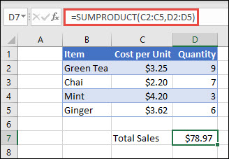
To create the formula using our sample list above, type =SUMPRODUCT(C2:C5,D2:D5) and press Enter. Each cell in column C is multiplied by its corresponding cell in the same row in column D, and the results are added up. The total amount for the groceries is $78.97.
To write a longer formula that gives you the same result, type =C2*D2+C3*D3+C4*D4+C5*D5 and press Enter. After pressing Enter, the result is the same: $78.97. Cell C2 is multiplied by D2, and its result is added to the result of cell C3 times cell D3 and so on.
Example 2
The following example uses SUMPRODUCT to return the total net sales by sales agent, where we have both total sales and expenses by agent. In this case, we’re using an Excel table, which uses structured references instead of standard Excel ranges. Here you’ll see that the Sales, Expenses, and Agent ranges are referenced by name.

The formula is: =SUMPRODUCT(((Table1[Sales])+(Table1[Expenses]))*(Table1[Agent]=B8)), and it returns the sum of all sales and expenses for the agent listed in cell B8.
Example 3
In this example, we want to return the total of a particular item sold by a given region. In this case, how many cherries did the East region sell?
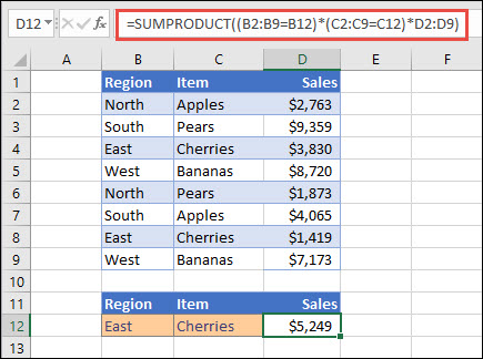
Here, the formula is: =SUMPRODUCT((B2:B9=B12)*(C2:C9=C12)*D2:D9). It first multiplies the number of occurrences of East by the number of matching occurrences of cherries. Finally, it sums the values of the corresponding rows in the Sales column. To see how Excel calculates this, select the formula cell, then go to Formulas > Evaluate Formula > Evaluate.
Need more help?
You can always ask an expert in the Excel Tech Community or get support in the Answers community.
See Also
Perform conditional calculations on ranges of cells
Sum based on multiple criteria with SUMIFS
Count based on multiple criteria with COUNTIFS
Average based on multiple criteria with AVERAGEIFS
Need more help?
Want more options?
Explore subscription benefits, browse training courses, learn how to secure your device, and more.
Communities help you ask and answer questions, give feedback, and hear from experts with rich knowledge.
SUMPRODUCT in Excel – is the favorite function of accountants, because it is most commonly used for the calculation of wages. Although it happens, it is useful in many other spheres.
You can guess by it name, that the team is responsible for the summation of compositions. The compositions in this case are considered either ranges or whole arrays.
The syntax function SUMPRODUCT
The arguments of the function SUMPRODUCT are arrays, that is to say the preset ranges. There can be as many as you like. Listing them through a semicolon, we set the number of arrays, which must first be multiplied, and then summed. The only condition is that the arrays must be equal in length and of the same type (that is, either all horizontal or all vertical ones).
The simplest example of using the function
To make it clear how and what the team believes, we consider the simple example. We have the table with the specified lengths and widths of the rectangles. We need to calculate the sum of the areas of all the rectangles. If you do not use this function, you will have to perform intermediate actions and calculate the area of each rectangle, and only then the sum — as we have done.
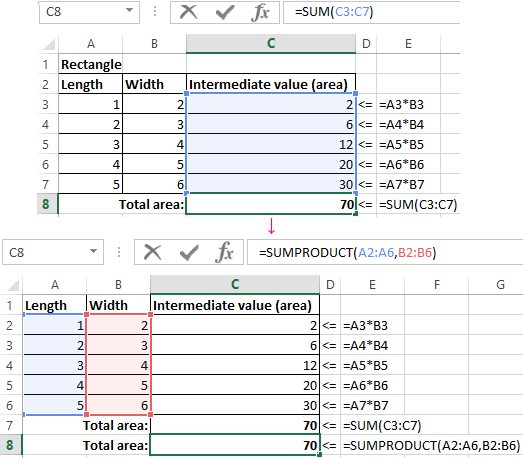
Pay attention that we did not need an array with subtotals. In the arguments of the function, we used only arrays of length and width, and the function automatically multiplied and summed them, yielding the same result = is 70.
SUMPRODUCT with the condition
The function SUMPRODUCT in its natural form is almost not used, because the calculation of the amount of works can rarely be useful in production. One of the popular applications of the SUMPRODUCT formula – is to output values that satisfying by specified conditions.
Let’s consider the example. We have the cost table for a small company for one month. It is necessary to calculate the total amount spent for January and February for all items of expenditure.
For calculating of the costs for the chancellery in January-month, we use our function and specify in the beginning two conditions. Each of them we enclose in parentheses, and between conditions need to put the «asterisk» sign, meaning the «and» union. We get the following command syntax:
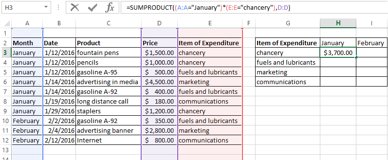
- A:A = «January») — the first condition;
- E:E = «chancery» — the second condition;
- D:D – is the array, from which the total amount is displayed.
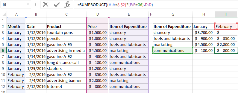
As a result, it turned out that in January 3,700 dollars were spent for office supplies. We will extend the formula to the remaining lines and replace in each of them the conditions (replacing the month or the item of expenditure).
The comparison in SUMPRODUCT
One of the conditions when using the SUMPRODUCT command can be a comparison. Let’s consider at once on the example and suppose that we need to calculate not just all office expenses for January, but only those that were less than 1000 dollars (let’s call them «the small expenses»). We prescribe to the function with the same arguments, but in addition we place the comparison operator. In this case, it looks like D:D >= 1000. The command issues to the following response: 1000.
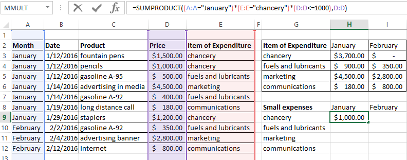
And indeed, this is the thousand that was spent in January on the pencils. We also set the comparison condition, and when the value was automatically returned and the function gave us such the response.
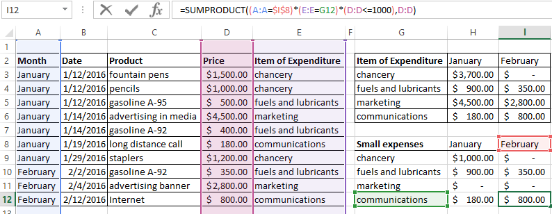
Download all examples SUMPRODUCT in Excel.
We extend the formula to the remaining cells, partially replacing to the information. We discover how much money was spent in January and February for small expenses for each cost item.
The SUMPRODUCT function multiplies arrays together and returns the sum of products. If only one array is supplied, SUMPRODUCT will simply sum the items in the array. Up to 30 ranges or arrays can be supplied.
When you first encounter SUMPRODUCT, it may seem boring, complex, and even pointless. But SUMPRODUCT is an amazingly versatile function with many uses. Because it will handle arrays gracefully, you can use it to process ranges of cells in clever, elegant ways.
Worksheet shown
In the worksheet shown above, SUMPRODUCT is used to calculate a conditional sum in three separate formulas:
I5=SUMPRODUCT(--(C5:C14="red"),F5:F14) //
I6=SUMPRODUCT(--(B5:B14="tx"),--(C5:C14="red"),F5:F14)
I7=SUMPRODUCT(--(B5:B14="co"),--(C5:C14="blue"),F5:F14)
The results are visible in cells I5, I6, and I7. The article below explains how SUMPRODUCT can be used to calculate these kind of conditional sums, and the purpose of the double negative (—).
Classic SUMPRODUCT example
The «classic» SUMPRODUCT example illustrates how you can calculate a sum directly without a helper column. For example, in the worksheet below, you can use SUMPRODUCT to get the total of all numbers in column F without using column F at all:

To perform this calculation, SUMPRODUCT uses values in columns D and E directly like this:
=SUMPRODUCT(D5:D14,E5:E14) // returns 1612
The result is the same as summing all values in column F. The formula is evaluated like this:
=SUMPRODUCT(D5:D14,E5:E14)
=SUMPRODUCT({10;6;14;9;11;10;8;9;11;10},{15;18;15;16;18;18;15;16;18;16})
=SUMPRODUCT({150;108;210;144;198;180;120;144;198;160})
=1612
This use of SUMPRODUCT can be handy, especially when there is no room (or no need) for a helper column with an intermediate calculation. However, the most common use of SUMPRODUCT in the real world is to apply conditional logic in situations that require more flexibility than functions like SUMIFS and COUNTIFS can offer.
SUMPRODUCT for conditional sums and counts
Assume you have some order data in A2:B6, with State in column A, Sales in column B:
| A | B | |
| 1 | State | Sales |
| 2 | UT | 75 |
| 3 | CO | 100 |
| 4 | TX | 125 |
| 5 | CO | 125 |
| 6 | TX | 150 |
Using SUMPRODUCT, you can count total sales for Texas («TX») with this formula:
=SUMPRODUCT(--(A2:A6="TX"))
And you can sum total sales for Texas («TX») with this formula:
=SUMPRODUCT(--(A2:A6="TX"),B2:B6)
Note: The double-negative is a common trick used in more advanced Excel formulas to coerce TRUE and FALSE values into 1’s and 0’s.
For the sum example above, here is a virtual representation of the two arrays as first processed by SUMPRODUCT:
| array1 | array2 |
| FALSE | 75 |
| FALSE | 100 |
| TRUE | 125 |
| FALSE | 125 |
| TRUE | 150 |
Each array has 5 items. Array1 contains the TRUE / FALSE values that result from the expression A2:A6=»TX», and array2 contains the values in B2:B6. Each item array1 will be multiplied by the corresponding item in the array.2 However, in the current state, the result will be zero because the TRUE and FALSE values in array1 will be evaluated as zero. We need the items in array1 to be numeric, and this is where the double-negative is useful.
Double negative (—)
The double negative (—) is one of several ways to coerce TRUE and FALSE values into their numeric equivalents, 1 and 0. Once we have 1s and 0s, we can perform various operations on the arrays with Boolean logic. The table below shows the result in array1, based on the formula above, after the double negative (—) has changed the TRUE and FALSE values to 1s and 0s.
| array1 | array2 | Product | ||
| 0 | * | 75 | = | 0 |
| 0 | * | 100 | = | 0 |
| 1 | * | 125 | = | 125 |
| 0 | * | 125 | = | 0 |
| 1 | * | 150 | = | 150 |
| Sum | 275 |
Translating the table above into arrays, this is how the formula is evaluated:
=SUMPRODUCT({0,0,1,0,1},{75,100,125,125,150})
SUMPRODUCT then multiples array1 and array2 together, resulting in a single array:
=SUMPRODUCT({0,0,125,0,150})
Finally, SUMPRODUCT returns the sum of all values in the array, 275. This example expands on the ideas above with more detail.
Abbreviated syntax in array1
You will often see the formula described above written in a different way like this:
=SUMPRODUCT((A2:A6="TX")*B2:B6) // returns 275
Norice all calculations have been moved into array1. The result is the same, but this syntax provides several advantages. First, the formula is more compact, especially as the logic becomes more complex. This is because the double negative (—) is no longer needed to convert TRUE and FALSE values — the math operation of multiplication (*) automatically converts the TRUE and FALSE values from (A2:A6=»TX») to 1s and 0s. But the most important advantage is flexibility. When using separate arguments, the operation is always multiplication, since SUMPRODUCT returns the sum of products. This limits the formula to AND logic, since multiplication corresponds to addition in Boolean algebra. Moving calculations into one argument means you can use addition (+) for OR logic, in any combination. In other words, you can choose your own math operations, which ultimately dictate the logic of the formula. See example here.
With the above advantages in mind, there is one disadvantage to the abbreviated syntax. SUMPRODUCT is programmed to ignore the errors that result from multiplying text values in arrays given as separate arguments. This can be handy in certain situations. With the abbreviated syntax, this advantage goes away, since the multiplication happens inside a single array argument. In this case, the normal behavior applies: text values will create #VALUE! errors.
Note: Technically, moving calculations into array1 creates an «array operation» and SUMPRODUCT is one of only a few functions that can handle an array operation natively without Control + Shift + Enter in Legacy Excel. See Why SUMPRODUCT? for more details.
Ignoring empty cells
To ignore empty cells with SUMPRODUCT, you can use an expression like range<>»». In the example below, the formulas in F5 and F6 both ignore cells in column C that do not contain a value:
=SUMPRODUCT(--(C5:C15<>"")) // count
=SUMPRODUCT(--(C5:C15<>"")*D5:D15) // sum

SUMPRODUCT with other functions
SUMPRODUCT can use other functions directly. You might see SUMPRODUCT used with the LEN function to count total characters in a range, or with functions like ISBLANK, ISTEXT, etc. These are not normally array functions, but when they are given a range, they create a «result array». Because SUMPRODUCT is built to work with arrays, it able to perform calculations on the arrays directly. This can be a good way to save space in a worksheet, by eliminating the need for a «helper» column.
For example, assume you have 10 different text values in A1:A10 and you want to count the total characters for all 10 values. You could add a helper column in column B that uses this formula: LEN(A1) to calculate the characters in each cell. Then you could use SUM to add up all 10 numbers. However, using SUMPRODUCT, you can write a formula like this:
=SUMPRODUCT(LEN(A1:A10))
When used with a range like A1:A10, LEN will return an array of 10 values. Then SUMPRODUCT will simply sum all values and return the result, with no helper column needed.
See examples below of many other ways to use SUMPRODUCT.
Arrays and Excel 365
This is a confusing topic, but it must be addressed. The SUMPRODUCT function can be used to create array formulas that don’t require control + shift + enter. This is a key reason that SUMPRODUCT has been so widely used to create more advanced formulas. One problem with array formulas is that they usually return incorrect results if they are not entered with control + shift + enter. This means if someone forgets to use CSE when checking or adjusting a formula, the result may suddenly change, even though the actual formula did not change. Using SUMPRODUCT means the formulas will work in any version of Excel without special handling.
In Excel 365, the formula engine handles arrays natively. This means you can often use the SUM function in place of SUMPRODUCT in an array formula with the same result and no need to enter the formula in a special way. However, if the same formula is opened in an earlier version of Excel, it will require control + shift + enter.
The bottom line is that SUMPRODUCT is a safer option if a worksheet will be used in any version of Excel before Excel 365, even if the worksheet was created in Excel 365. For more details and examples, see Why SUMPRODUCT?
Notes
- SUMPRODUCT treats non-numeric items in arrays as zeros.
- Array arguments must be the same size. Otherwise, SUMPRODUCT will generate a #VALUE! error value.
- Logical tests inside arrays will create TRUE and FALSE values. In most cases, you’ll want to coerce these to 1’s and 0’s.
- SUMPRODUCT can often use the result of other functions directly (see formula examples below)
SUMPRODUCT Function in Excel
The SUMPRODUCT excel function multiplies the numbers of two or more arrays and sums up the resulting products. An array is a range of cells supplied as an argument to the SUMPRODUCT function. A product is the output of the multiplication of two numbers.
For example, a worksheet consists of numeric values in columns A and B. They are listed as follows:
Column A
- Cell A1 contains 3
- Cell A2 contains 4
- Cell A3 contains 5
Column B
- Cell B1 contains 2
- Cell B2 contains 6
- Cell B3 contains 1
The formula “=SUMPRODUCT(A1:A3,B1:B3)” returns 35. The given formula has calculated the output as (3*2)+(4*6)+(5*1)=35. Hence, the SUMPRODUCT multiplies the respective values of the specified arrays and sums up the resulting products.
Had there been only one range, A1:A3, the formula “=SUMPRODUCT(A1:A3)” would have returned 12. This is because, in case of one array, the SUMPRODUCT excel function returns the sum of the values of the single array.
Even though the SUMPRODUCT works on arrays, it does not require the CSE shortcut (Ctrl+Shift+Enter) to operate. Rather, the “Enter” key is pressed to perform the calculations.
The SUMPRODUCT function is categorized under the Math and Trigonometry functions of Excel. To extend the functionality of the SUMPRODUCT function, it can be combined with several other functions of Excel.
Table of contents
- SUMPRODUCT Function in Excel
- Syntax of the SUMPRODUCT Formula in Excel
- Sumproduct Excel Function Examples
- Example #1–Multiply and Add Numbers
- Example #2–Multiply and Add Based on a Criterion (Condition)
- Example #3–Mutliply and Add to Find the Weighted Average
- Example #4–Multiply and Add Based on Multiple Criteria (Conditions)
- The Properties of the SUMPRODUCT Excel Function
- Frequently Asked Questions
- SUMPRODUCT Excel Function Video
- Recommended Articles
Syntax of the SUMPRODUCT Formula in Excel
The syntax of the SUMPRODUCT excel function is shown in the following image:
The SUMPRODUCT function accepts the following arguments:
- array1: This is the first array (range) whose values are to be multiplied and then added.
- array2: This is the second array (range) whose values are to be multiplied and then added.
- array3: This is the third array (range) whose values are to be multiplied and then added.
The “array1” argument is mandatory. The “array2,” “array3,” and the subsequent array arguments are optional.
Note: By default, the SUMPRODUCT function in excel multiplies numbers. However, it can also perform addition, subtraction, and division. For such arithmetic operations, place the relevant operator like “plus” (+), “minus” (-), or “forward slash” (/) between the array arguments supplied to the SUMPRODUCT function.
Sumproduct Excel Function Examples
Let us consider some examples to understand the working of the SUMPRODUCT function of Excel.
You can download this SUMPRODUCT Function Excel Template here – SUMPRODUCT Function Excel Template
Example #1–Multiply and Add Numbers
The succeeding image shows the prices (in $ in column C) and the number of units sold (column B) of 10 products. Calculate the total sales revenueSales revenue refers to the income generated by any business entity by selling its goods or providing its services during the normal course of its operations. It is reported annually, quarterly or monthly as the case may be in the business entity’s income statement/profit & loss account.read more generated by the products A to J.
Step 1: Enter the following formula in cell B15.
“=SUMPRODUCT($B$5:$B$14,$C$5:$C$14)”
Step 2: Press the “Enter” key. The output is $200,600. Hence, the total sales revenue generated by the given products (A to J) is $200,600.
For simplicity, we have shown the formula in cell B15 and given the result in cell C15.
Note: The absolute referencesAbsolute reference in excel is a type of cell reference in which the cells being referred to do not change, as they did in relative reference. By pressing f4, we can create a formula for absolute referencing.read more (shown by the dollar symbol) in the SUMPRODUCT formula ensure that the formula does not change on being copied.

Explanation: The given SUMPRODUCT formula multiplies the values of column B with the corresponding values of column C. Thereafter, the products obtained are summed up.
The SUMPRODUCT formula (entered in step 1) works as follows:
(20*1300)+(10*1500)+(17*1000)+(14*1300)+(15*1700)+(14*1200)+(15*1100)+(18*1300)+(16*1500)+(13*1400)
=26000+15000+17000+18200+25500+16800+16500+23400+24000+18200
=200600
Hence, the output of the SUMPRODUCT formula is $200,600.
Example #2–Multiply and Add Based on a Criterion (Condition)
The succeeding image shows the sales revenue (in $ in column D) generated by the different regions (column C) for twelve months. Calculate the total sales revenue generated by the West region for the given period.
Step 1: Enter the following formula in cell C32.
“=SUMPRODUCT(–($C$20:$C$31=”West”),$D$20:$D$31)”
Step 2: Press the “Enter” key. The output is $1,500. Hence, the total sales revenue generated by the West region for the period of twelve months is $1,500.
For simplicity, the SUMPRODUCT formula is shown in cell C32 and the result is given in cell D32.

Explanation: The formula $C$20:$C$31=”West” returns a series of logical values, true or false. It returns true for all cells (of the range C20:C31) that contain “West.” For cells containing values other than “West” (like North or South), the formula returns false.
The unary operator or the double negative symbol (–) converts the true and false values into 1 and 0 respectively. Had we not used the unary operator, the SUMPRODUCT function in excel would have treated the non-numeric values (of column C) as zeroes.
The first array of the SUMPRODUCT function results from the formula $C$20:$C$31=”West”. This array consists of only ones (1) and zeroes (0). The second array of the SUMPRODUCT function is $D$20:$D$31.
Since all cells (of the range C20:C31) containing “West” evaluate to 1, the SUMPRODUCT excel function works as follows:
(1*100)+(0*500)+(0*300)+(1*400)+(0*100)+(1*500)+(0*300)+(0*400)+(1*100)+(0*500)+(0*300)+(1*400)
=100+0+0+400+0+500+0+0+100+0+0+400
=1500
Hence, the output of the SUMPRODUCT formula is $1,500.
Example #3–Mutliply and Add to Find the Weighted Average
The succeeding image shows the completion percentages (column C) of 10 projects of an organization. With these percentages, one can figure out the extent to which the respective project has been completed. The priority rating (column D) is the weight assigned to a project.
Calculate the weighted average of the given projects with the help of the SUMPRODUCT excel function.
Step 1: Enter the following SUMPRODUCT formula.
“=SUMPRODUCT(C36:C46,D36:D46)/SUM(D36:D46)”
Step 2: Press the “Enter” key. The output is 55.8%. Hence, the weighted average is 55.8%.

Explanation: For calculating the weighted average, the following calculations are performed in the given sequence:
- The completion percentages (C36:C46) are multiplied by the weights (D36:D46).
- The resulting products (obtained in step a) are added.
- The answer obtained (in step b) is divided by the sum of the weights [SUM(D36:D46)].
The SUMPRODUCT formula (entered in step 1) works as follows:
[(0*0)+(0.5*2)+(0.6*3)+(0.65*1)+(0.4*1)+(0.5*2)+(0.6*4)+(0.5*1)+(0.6*4)+(0.65*4)+(0.4*3)]/(0+2+3+1+1+2+4+1+4+4+3)
=(0+1+1.8+0.65+0.4+1+2.4+0.5+2.4+2.6+1.2)/25
=13.95/25
=0.558 or 55.8%
Hence, the weighted average is 55.8%.
Note: The non-numeric values in cells C36 and D36 are treated as zeroes by the given SUMPRODUCT formula.
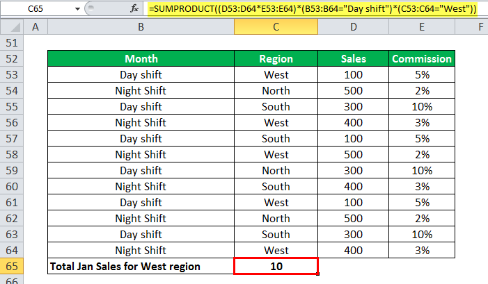
Example #4–Multiply and Add Based on Multiple Criteria (Conditions)
The succeeding image shows the sales revenues (in $ in column D) generated by the employees of different regions (column C). On every sale, a percentage of commission (column E) is earned by the employees.
Further, the employees work in two shifts, the day shift and the night shift. The entire dataset relates to the month of January of a particular year.
Calculate the total commission (in $) paid to the employees of the West region who are working in day shifts.
Step 1: Enter the following formula in cell C65.
“=SUMPRODUCT((D53:D64*E53:E64)*(B53:B64=”Day shift”)*(C53:C64=”West”))”
Step 2: Press the “Enter” key. The output is $10.
Explanation: The formula B53:B64=”Day shift” helps find the cells (in the range B53:B64) that contain the words “day shift.” If a cell of column B contains “day shift,” the result is true. Otherwise, the result is false.
Likewise, the formula C53:C64=”West” returns true or false depending on the value of cells in the given range (C53:C64). It returns true for all cells of column C that contain “West.” If the cells contain values other than “West” (like North or South), this formula returns false.
Since there is no unary operator (–) preceding these formulas, the true and false values are not converted into binary digits (0 and 1).
The SUMPRODUCT formula (entered in step 1) consists of multiple criteria. The criteria for columns B and C are “day shift” and “West” respectively. From the given dataset, only rows 53 and 61 satisfy the stated criteria.
Therefore, the SUMPRODUCT excel formula multiplies and adds the corresponding values of columns D and E for rows 53 and 61 only.
Row 53 contains 100 and 5% in cells D53 and E53 respectively. Likewise, row 61 also contains 100 and 5% in cells D61 and E61 respectively. These numbers are multiplied and then added.
The SUMPRODUCT formula works as follows:
(100*5%)+(100*5%)
=10
Hence, the employees working in day shifts and belonging to the West region are paid a total commission of $10.
The Properties of the SUMPRODUCT Excel Function
The features of the SUMPRODUCT excel function are listed as follows:
- The minimum number of arrays to be supplied to the SUMPRODUCT function is 1. If a single array is supplied, the function returns the sum of all the items of this array.
- The maximum number of arrays that can be specified is 255 in Excel 2007 and the newer versions. In the older Excel versions, the maximum limit of arrays is fixed at 30.
- All array arguments must have the same number of rows and columns. If not, the SUMPRODUCT function returns the #VALUE error#VALUE! Error in Excel represents that the reference cell the user has either entered an incorrect formula or used a wrong data type (mostly numerical data). Sometimes, it is difficult to identify the kind of mistake behind this error.read more.
- The SUMPRODUCT excel function treats the non-numeric entries of an array as zeroes.
- The logical testsA logical test in Excel results in an analytical output, either true or false. The equals to operator, “=,” is the most commonly used logical test.read more within arrays evaluate to the Boolean values, true or false. These values can be converted to 1 and 0 with the help of the unary operator (–).
Note: The SUMPRODUCT can be used as a VBA functionVBA functions serve the primary purpose to carry out specific calculations and to return a value. Therefore, in VBA, we use syntax to specify the parameters and data type while defining the function. Such functions are called user-defined functions.read more. For instance, a code can be created as follows:
Sub ABC()
MsgBox Evaluate(“=SUMPRODUCT(($A$1:$A$5=””Tanuj””)*($B$1:$B$5))”)
End Sub
The values of array A1:A5 that evaluate to “Tanuj” are multiplied by the corresponding values of the array B1:B5. The resulting products are then summed up.
Frequently Asked Questions
1. Define the SUMPRODUCT function of Excel.
The SUMPRODUCT function multiplies the numerical values of two or more arrays. The resulting products are then added. Further, it is possible to specify one or more conditions (criteria) based on which the function returns an output.
Besides multiplication, the SUMPRODUCT excle function can also perform addition, subtraction and division.
The syntax of the SUMPRODUCT excel function is stated as follows:
“SUMPRODUCT(array1,[array2],[array3],…)”
The arguments “array1,” “array2,” and “array3” are the range of values that are to be multiplied and then added. “Array1” is mandatory, while the subsequent array arguments are optional.
In the modern Excel versions, a minimum of 1 and a maximum of 255 arrays can be supplied to the SUMPRODUCT function. In case of a single array, the function returns the sum of the range supplied.
2. How does the SUMPRODUCT excel function work and when is it used in Excel?
The SUMPRODUCT function in excel works as follows:
a. Arrays, separated with commas, are supplied to the function.
b. The function evaluates the conditions, if any.
c. Once the “Enter” key is pressed, the function performs the calculations and returns a numeric output.
The SUMPRODUCT function is used in the following situations:
a. It is used when two or more numbers need to be multiplied and added with a single formula.
b. It is used to count values satisfying the specified criteria.
c. It is used to calculate the weighted average.
d. It is used when multiplication and addition operations need to be performed after one or more conditions have been met.
e. It is used when different arithmetic operations like addition, division, and subtraction are to be performed.
Note: For performing addition, division, and subtraction, place the respective operator like “+,” “/” or “-” between the array arguments supplied to the SUMPRODUCT formula of Excel.
For instance, the formula “=SUMPRODUCT(A2:A5-B2:B5) subtracts the numbers in the first range (A2:A5) from the numbers in the second range (B2:B5). The differences thus obtained are then added.
3. How to use the SUMPRODUCT function with multiple conditions?
When multiple conditions are entered in the SUMPRODUCT excel function, it evaluates each condition before returning an output. The SUMPRODUCT function works with both, the AND and the OR logic.
For example, a cake manufacturer of USA wants to find out the number of buyers in Chicago and Houston. For this, a dataset consisting of two flavors of cake (pineapple and chocolate) is studied. The worksheet contains the following entries:
The text “flavors” is displayed in cell A1. This list contains the following items:
• Cells A2, A5, A6, and A7 contain Pineapple.
• Cells A3 and A4 contain Chocolate.
The text “cities” is displayed in cell B2. This list contains the following items:
• Cells B2, B4, B6, and B7 contain Chicago.
• Cells B3 and B5 contain Houston.
The text “number of buyers” is displayed in cell C3. This list contains the following items:
• Cell C2 contains 11,020.
• Cell C3 contains 10,900.
• Cell C4 contains 20,765.
• Cell C5 contains 15,083.
• Cell C6 contains 21,032.
• Cell C7 contains 12,098.
SUMPRODUCT with AND logic
The AND logic works by using the asterisk (*). Let us calculate the total number of buyers of pineapple cake in Chicago.
a. Enter the formula “=SUMPRODUCT((A2:A7=”pineapple”)*(B2:B7=”chicago”)*C2:C7)” in any cell, say E2.
b. Press the “Enter” key.
The output is 44,150. The SUMPRODUCT function looks for “pineapple” in column A (A2:A7) and “Chicago” in column B (B2:B7). The entries which are equal to both “pineapple” and “Chicago” are summed up.
So, 11020+21032+12098=44150
Hence, the pineapple cake was purchased by 44,150 buyers in Chicago.
SUMPRODUCT with OR logic
The OR logic works by using the plus (+) sign. Let us calculate the number of buyers who have either purchased the pineapple cake or belong to Chicago.
a. Enter the formula “=SUMPRODUCT((A2:A7=”pineapple”)+(B2:B7=”chicago”),C2:C7)” in cell F2.
b. Press the “Enter” key.
The output is 124,148. The SUMPRODUCT function searches for “pineapple” in the first range (A2:A7) and “Chicago” in the second range (B2:B7). The entries which are equal to either “pineapple” or “Chicago” are summed up.
In other words, the SUMPRODUCT function counts an entry for which any of the conditions (A2:A7=”pineapple” or B2:B7=”chicago”) evaluates to true.
So, (2*11020)+(1*20765)+(1*15083)+(2*21032)+(2*12098)=124,148.
The SUMPRODUCT excel function counts “pineapple” as one entry and “Chicago” as another entry. If a row has both “pineapple” and “Chicago,” it is counted as two entries. There are a total of 8 cells which have either “pineapple” or “Chicago.”
Rows 2, 6, and 7 have both “pineapple” and “Chicago.” So, for these rows, the corresponding figures of column C are multiplied by 2. Rows 4 and 5 have “Chicago” and “pineapple” respectively. So, for these rows, the respective figures of column C are multiplied by 1.
Hence, a total of 124,148 buyers either purchased the pineapple cake or belong to Chicago.
Note: The SUMPRODUCT function can also work for both AND and OR logic simultaneously.
SUMPRODUCT Excel Function Video
Recommended Articles
This has been a guide to SUMPRODUCT in Excel. Here we discuss how to use SUMPRODUCT Function along with step by step excel example.. You may also look at these useful functions of Excel-
- SUMPRODUCT with Multiple CriteriaIn Excel, using SUMPRODUCT with several Criteria allows you to compare different arrays using multiple criteria.read more
- SUBTOTAL Excel FunctionThe SUBTOTAL excel function performs different arithmetic operations like average, product, sum, standard deviation, variance etc., on a defined range.read more
- AGGREGATE FunctionAGGREGATE Function in excel returns the aggregate of a given data table or data lists.read more
- SIGN Excel FunctionThe sign function in excel is a Math/Trig function that returns the sign (-1, 0 or +1) of the numerical argument supplied to it.read more
- Redo Shortcut in ExcelIn Excel, we have an option named “Undo” that we may use by pressing Ctrl + Z. When we undo an action but subsequently realize it was not a mistake, we can cancel the undo action and return to the original point, using «Redo.»read more
Home > Data Science > What is SUMPRODUCT in Excel: Complete Guide
Microsoft Office Suite is one of Microsoft’s most popular software package offerings, with applications for word processing, spreadsheets, and other functions. A part of the Office Suite, Microsoft Excel is a widely used data storage and analysis program. It is a spreadsheet program with various functions and formulas that enables users to perform calculations and analyses on numerical data.
Unlike its word processor counterpart (Microsoft Word), Excel can be quite challenging to navigate and grasp, mainly because of the numerous formulas, functions, and features it offers.
This article will explore the SUMPRODUCT function in Excel and its uses in simplifying numerical data analysis.
Learn data science courses online from the World’s top Universities. Earn Executive PG Programs, Advanced Certificate Programs, or Masters Programs to fast-track your career.
Explore our Popular Data Science Courses
What is the SUMPRODUCT function/SUMPRODUCT formula in Excel?
The SUMPRODUCT function in Excel returns the summation of products of corresponding arrays or ranges. We can use the function to multiply two or more arrays together and get the sum of products. An array or range in Excel is a collection of selected cells, either rows or columns of values or a combination of rows and columns of values. SUMPRODUCT in Excel is a highly versatile function. Although its default operation is multiplication, we can also use it for addition, subtraction, and division.
Syntax of the SUMPRODUCT Function in Excel
The syntax for basic use of the Excel SUMPRODUCT function for the default operation (multiplication) is as follows:
=SUMPRODUCT(array1, [array2], [array3], …)
Example:
=SUMPRODUCT(B2:B5, C2:C5)
Syntax arguments
The first array argument (array1) is mandatory in the syntax and includes the components we want to multiply then add. However, [array2], [array3], and so on are optional and have values we want to multiply and then add.
Using other arithmetic operators
If we want to perform other arithmetic operations apart from multiplication, use SUMPRODUCT as usual and replace the commas between the array arguments with the arithmetic operators (+, -, *, /) we wish to use.
Example of SUMPRODUCT Function in Excel
Below is an example showing the basic use of the Excel SUMPRODUCT function:

Source
How to use the SUMPRODUCT function in Excel?
We’ll look at some examples to understand how to use the Excel SUMPRODUCT function.
Example 1
Suppose we have the following data:

We want to find out the total amount spent. So, we will use the SUMPRODUCT function as follows:

The SUMPRODUCT function performs the following calculation: (10*20) + (20*10) + (15*12) + (5*25) + (10*20) + (6*5) = 935

Example 2
Now, consider the following data:

We want to find out the total sales in the north region. So, we will use the SUMPRODUCT function as follows:

Here, the double negative sign (–) in the syntax converts the TRUE and FALSE values into 0s and 1s.
Below is a virtual representation of the two arrays as processed by the SUMPRODUCT function if we do not use the double negative signs:

The first array contains the TRUE or FALSE values resulting from the argument B1:B7=”North,” and the second array includes the values of C1:C7. Thus, the SUMPRODUCT function multiplies each item in the first array with the corresponding item in the second array.
The SUMPRODUCT function will return zero in this state because it treats the TRUE and FALSE values as zeroes. So, we need to convert the items in the first array into numeric values( 0s and 1s). Hence, we use the double negative signs that treat TRUE and FALSE as 1 and 0, respectively.

The result is as follows:

Example 3

Look at the following data:
Here, we will use the SUMPRODUCT function to calculate the weighted average where each value has been assigned a weight (in this case, the quantity). The SUMPRODUCT formula for calculating the weighted average is as follows:

The result is:

Using the SUMPRODUCT Function to Calculate Specific Character Occurences in a Range
Apart from purely numeric calculations, we can also use the SUMPRODUCT formula in Excel to calculate the occurrence of specific characters in a range of cells. The general syntax for it is:
=SUMPRODUCT(LEN(rng)-LEN(SUBSTITUTE(rng,txt,””)))
In the syntax above, rng represents the range of cells containing words, and txt represents the character we want to count.
Consider the following example:

To count the total number of the character “a”, we will use the syntax:
=SUMPRODUCT(LEN(A2:A6)-LEN(SUBSTITUTE(A2:A6,”a”,””)))

The result:

Here, SUBSTITUTE takes away all the “a”s from the text in each cell of the range, and then LEN finds out the text length without the “a”s. The number is then deducted from the initial text length with “a”s.
Since we are using the SUMPRODUCT function, the above calculation results give an array with one item (a number) in each cell of the range. Thus, we have an array of character counts with one count in every cell. The SUMPRODUCT function then adds the numbers in the list and returns the total for all the cells in the range.
Since SUBSTITUTE is a case-sensitive function, it will match the case while performing calculations. So, if we want to count both the lower and uppercase instances of a specific character, we will modify the syntax to convert the text to uppercase before the substitution happens. The modified syntax will be:
=SUMPRODUCT(LEN(rng)-LEN(SUBSTITUTE(UPPER(rng),TXT,””)))
Using the SUMPRODUCT Function to Count Specified Words in a Range
We can use the following SUMPRODUCT formula to count the occurrence of a specific word in a range of cells. The generic syntax is:
=SUMPRODUCT((LEN(rng)-LEN(SUBSTITUTE(rng,txt,””)))/LEN(txt))
In the syntax, rng represents the cell range we want to check, and txt is the word or substring we wish to count.
Consider the following example:

To calculate the total count of the word “Jill,” we will use the syntax:
=SUMPRODUCT((LEN(A2:A5)-LEN(SUBSTITUTE(A2:A5,D2,””)))/LEN(D2))

The result:

SUBSTITUTE removes the substring (Jill) from the initial text for every cell in the array, and then LEN computes the text length minus the substring. The number is then deducted from the initial text length to get the number of characters removed by SUBSTITUTE. The function then divides the number of removed characters by the length of the substring to get the number of times the substring appeared in the initial text (this is the list of items/array).
The SUMPRODUCT function finally adds up all the items in the array to return the total instances of the substring in the range of cells.
Points to Remember While Using the SUMPRODUCT Function
1. The array arguments in the SUMPRODUCT function must have the same dimensions. If not, the function returns the #VALUE! error. An example has been shown below. Here, the ranges (B2:B8, C2:C7) are not the same.
 2. The SUMPRODUCT function treats non-numeric array components as if they were zeroes.

3. The SUMPRODUCT function returns the same result as the SUM function on applying a single range.
 4. The SUMPRODUCT function accepts up to 255 arguments in Excel 2016, 2013, 2010, and 2007 versions and up to 30 in earlier ones.
5. Logical test components inside arrays create TRUE and FALSE values. Thus, converting them into numeric values (0s and 1s) is common.
Read our popular Data Science Articles
Learn Excel with upGrad Data Analytics Certificate Program
Are you a working professional looking for a break in the data analytics field? Then here’s your chance to learn and train with upGrad’s Data Analytics Certificate Program powered by Fullstack Academy.
Highlights of the 9-month blended program (live+online):
- 200+ learning hours
- Fullstack Academy live training
- Certificate from Caltech
- Tableau and AWS certification preparation
- 1:1 career mentorship sessions
- Peer learning and industry networking
- Comprehensive coverage of data analytics tools and programming languages (including Excel)
Sign up today to book your seat!
Is there a limit on SUMPRODUCT in Excel?
The SUMPRODUCT function accepts up to 255 arguments in Excel 2016, 2013, 2010, and 2007 and up to 30 in older versions.
What is the difference between SUMIFs and SUMPRODUCT?
While SUMPRODUCT calculates the total value of the products from multiple arrays or ranges of the same dimensions, SUMIFS sums cells that meet various criteria and occur in a single range. Thus, SUMPRODUCT is mathematical calculation-based, whereas SUMIFS is more logic-based
Why does SUMPRODUCT return value?
same dimension or if one or more cells in the selected range contain text.
Want to share this article?
