
From Wikipedia, the free encyclopedia
In natural language processing (NLP), a word embedding is a representation of a word. The embedding is used in text analysis. Typically, the representation is a real-valued vector that encodes the meaning of the word in such a way that words that are closer in the vector space are expected to be similar in meaning.[1] Word embeddings can be obtained using language modeling and feature learning techniques, where words or phrases from the vocabulary are mapped to vectors of real numbers.
Methods to generate this mapping include neural networks,[2] dimensionality reduction on the word co-occurrence matrix,[3][4][5] probabilistic models,[6] explainable knowledge base method,[7] and explicit representation in terms of the context in which words appear.[8]
Word and phrase embeddings, when used as the underlying input representation, have been shown to boost the performance in NLP tasks such as syntactic parsing[9] and sentiment analysis.[10]
Development and history of the approach[edit]
In Distributional semantics, a quantitative methodological approach to understanding meaning in observed language, word embeddings or semantic vector space models have been used as a knowledge representation for some time.[11] Such models aim to quantify and categorize semantic similarities between linguistic items based on their distributional properties in large samples of language data. The underlying idea that «a word is characterized by the company it keeps» was proposed in a 1957 article by John Rupert Firth,[12] but also has roots in the contemporaneous work on search systems[13] and in cognitive psychology.[14]
The notion of a semantic space with lexical items (words or multi-word terms) represented as vectors or embeddings is based on the computational challenges of capturing distributional characteristics and using them for practical application to measure similarity between words, phrases, or entire documents. The first generation of semantic space models is the vector space model for information retrieval.[15][16][17] Such vector space models for words and their distributional data implemented in their simplest form results in a very sparse vector space of high dimensionality (cf. Curse of dimensionality). Reducing the number of dimensions using linear algebraic methods such as singular value decomposition then led to the introduction of latent semantic analysis in the late 1980s and the Random indexing approach for collecting word cooccurrence contexts.[18][19][20][21] In 2000 Bengio et al. provided in a series of papers the «Neural probabilistic language models» to reduce the high dimensionality of words representations in contexts by «learning a distributed representation for words».[22][23]
A study published in NeurIPS (NIPS) 2002 introduced the use of both word and document embeddings applying the method of kernel CCA to bilingual (and multi-lingual) corpora, also providing an early example of self-supervised learning of word embeddings [24]
Word embeddings come in two different styles, one in which words are expressed as vectors of co-occurring words, and another in which words are expressed as vectors of linguistic contexts in which the words occur; these different styles are studied in (Lavelli et al., 2004).[25] Roweis and Saul published in Science how to use «locally linear embedding» (LLE) to discover representations of high dimensional data structures.[26] Most new word embedding techniques after about 2005 rely on a neural network architecture instead of more probabilistic and algebraic models, since some foundational work by Yoshua Bengio and colleagues.[27][28]
The approach has been adopted by many research groups after advances around year 2010 had been made on theoretical work on the quality of vectors and the training speed of the model and hardware advances allowed for a broader parameter space to be explored profitably. In 2013, a team at Google led by Tomas Mikolov created word2vec, a word embedding toolkit that can train vector space models faster than the previous approaches. The word2vec approach has been widely used in experimentation and was instrumental in raising interest for word embeddings as a technology, moving the research strand out of specialised research into broader experimentation and eventually paving the way for practical application.[29]
Polysemy and homonymy[edit]
Historically, one of the main limitations of static word embeddings or word vector space models is that words with multiple meanings are conflated into a single representation (a single vector in the semantic space). In other words, polysemy and homonymy are not handled properly. For example, in the sentence «The club I tried yesterday was great!», it is not clear if the term club is related to the word sense of a club sandwich, baseball club, clubhouse, golf club, or any other sense that club might have. The necessity to accommodate multiple meanings per word in different vectors (multi-sense embeddings) is the motivation for several contributions in NLP to split single-sense embeddings into multi-sense ones.[30][31]
Most approaches that produce multi-sense embeddings can be divided into two main categories for their word sense representation, i.e., unsupervised and knowledge-based.[32] Based on word2vec skip-gram, Multi-Sense Skip-Gram (MSSG)[33] performs word-sense discrimination and embedding simultaneously, improving its training time, while assuming a specific number of senses for each word. In the Non-Parametric Multi-Sense Skip-Gram (NP-MSSG) this number can vary depending on each word. Combining the prior knowledge of lexical databases (e.g., WordNet, ConceptNet, BabelNet), word embeddings and word sense disambiguation, Most Suitable Sense Annotation (MSSA)[34] labels word-senses through an unsupervised and knowledge-based approach, considering a word’s context in a pre-defined sliding window. Once the words are disambiguated, they can be used in a standard word embeddings technique, so multi-sense embeddings are produced. MSSA architecture allows the disambiguation and annotation process to be performed recurrently in a self-improving manner.[35]
The use of multi-sense embeddings is known to improve performance in several NLP tasks, such as part-of-speech tagging, semantic relation identification, semantic relatedness, named entity recognition and sentiment analysis.[36][37]
As of the late 2010s, contextually-meaningful embeddings such as ELMo and BERT have been developed.[38] Unlike static word embeddings, these embeddings are at the token-level, in that each occurrence of a word has its own embedding. These embeddings better reflect the multi-sense nature of words, because occurrences of a word in similar contexts are situated in similar regions of BERT’s embedding space.[39][40]
For biological sequences: BioVectors[edit]
Word embeddings for n-grams in biological sequences (e.g. DNA, RNA, and Proteins) for bioinformatics applications have been proposed by Asgari and Mofrad.[41] Named bio-vectors (BioVec) to refer to biological sequences in general with protein-vectors (ProtVec) for proteins (amino-acid sequences) and gene-vectors (GeneVec) for gene sequences, this representation can be widely used in applications of deep learning in proteomics and genomics. The results presented by Asgari and Mofrad[41] suggest that BioVectors can characterize biological sequences in terms of biochemical and biophysical interpretations of the underlying patterns.
Game design[edit]
Word embeddings with applications in game design have been proposed by Rabii and Cook[42] as a way to discover emergent gameplay using logs of gameplay data. The process requires to transcribe actions happening during the game within a formal language and then use the resulting text to create word embeddings. The results presented by Rabii and Cook[42] suggest that the resulting vectors can capture expert knowledge about games like chess, that are not explicitly stated in the game’s rules.
Sentence embeddings[edit]
The idea has been extended to embeddings of entire sentences or even documents, e.g. in the form of the thought vectors concept. In 2015, some researchers suggested «skip-thought vectors» as a means to improve the quality of machine translation.[43] A more recent and popular approach for representing sentences is Sentence-BERT, or SentenceTransformers, which modifies pre-trained BERT with the use of siamese and triplet network structures.[44]
Software[edit]
Software for training and using word embeddings includes Tomas Mikolov’s Word2vec, Stanford University’s GloVe,[45] GN-GloVe,[46] Flair embeddings,[36] AllenNLP’s ELMo,[47] BERT,[48] fastText, Gensim,[49] Indra,[50] and Deeplearning4j. Principal Component Analysis (PCA) and T-Distributed Stochastic Neighbour Embedding (t-SNE) are both used to reduce the dimensionality of word vector spaces and visualize word embeddings and clusters.[51]
Examples of application[edit]
For instance, the fastText is also used to calculate word embeddings for text corpora in Sketch Engine that are available online.[52]
Ethical Implications[edit]
Word embeddings may contain the biases and stereotypes contained in the trained dataset, as Bolukbasi et al. points out in the 2016 paper “Man is to Computer Programmer as Woman is to Homemaker? Debiasing Word Embeddings” that a publicly available (and popular) word2vec embedding trained on Google News texts (a commonly used data corpus), which consists of text written by professional journalists, still shows disproportionate word associations reflecting gender and racial biases when extracting word analogies (Bolukbasi et al. 2016). For example, one of the analogies generated using the aforementioned word embedding is “man is to computer programmer as woman is to homemaker”.[53]
The applications of these trained word embeddings without careful oversight likely perpetuates existing bias in society, which is introduced through unaltered training data. Furthermore, word embeddings can even amplify these biases (Zhao et al. 2017).[54] Given word embeddings popular usage in NLP applications such as search ranking, CV parsing and recommendation systems, the biases that exist in pre-trained word embeddings may have further reaching impact than we realize.
See also[edit]
- Brown clustering
- Distributional–relational database
References[edit]
- ^ Jurafsky, Daniel; H. James, Martin (2000). Speech and language processing : an introduction to natural language processing, computational linguistics, and speech recognition. Upper Saddle River, N.J.: Prentice Hall. ISBN 978-0-13-095069-7.
- ^ Mikolov, Tomas; Sutskever, Ilya; Chen, Kai; Corrado, Greg; Dean, Jeffrey (2013). «Distributed Representations of Words and Phrases and their Compositionality». arXiv:1310.4546 [cs.CL].
- ^ Lebret, Rémi; Collobert, Ronan (2013). «Word Emdeddings through Hellinger PCA». Conference of the European Chapter of the Association for Computational Linguistics (EACL). Vol. 2014. arXiv:1312.5542.
- ^ Levy, Omer; Goldberg, Yoav (2014). Neural Word Embedding as Implicit Matrix Factorization (PDF). NIPS.
- ^ Li, Yitan; Xu, Linli (2015). Word Embedding Revisited: A New Representation Learning and Explicit Matrix Factorization Perspective (PDF). Int’l J. Conf. on Artificial Intelligence (IJCAI).
- ^ Globerson, Amir (2007). «Euclidean Embedding of Co-occurrence Data» (PDF). Journal of Machine Learning Research.
- ^ Qureshi, M. Atif; Greene, Derek (2018-06-04). «EVE: explainable vector based embedding technique using Wikipedia». Journal of Intelligent Information Systems. 53: 137–165. arXiv:1702.06891. doi:10.1007/s10844-018-0511-x. ISSN 0925-9902. S2CID 10656055.
- ^ Levy, Omer; Goldberg, Yoav (2014). Linguistic Regularities in Sparse and Explicit Word Representations (PDF). CoNLL. pp. 171–180.
- ^ Socher, Richard; Bauer, John; Manning, Christopher; Ng, Andrew (2013). Parsing with compositional vector grammars (PDF). Proc. ACL Conf.
- ^ Socher, Richard; Perelygin, Alex; Wu, Jean; Chuang, Jason; Manning, Chris; Ng, Andrew; Potts, Chris (2013). Recursive Deep Models for Semantic Compositionality Over a Sentiment Treebank (PDF). EMNLP.
- ^ Sahlgren, Magnus. «A brief history of word embeddings».
- ^ Firth, J.R. (1957). «A synopsis of linguistic theory 1930–1955». Studies in Linguistic Analysis: 1–32. Reprinted in F.R. Palmer, ed. (1968). Selected Papers of J.R. Firth 1952–1959. London: Longman.
- ^ }Luhn, H.P. (1953). «A New Method of Recording and Searching Information». American Documentation. 4: 14–16. doi:10.1002/asi.5090040104.
- ^ Osgood, C.E.; Suci, G.J.; Tannenbaum, P.H. (1957). The Measurement of Meaning. University of Illinois Press.
- ^ Salton, Gerard (1962). «Some experiments in the generation of word and document associations». Proceeding AFIPS ’62 (Fall) Proceedings of the December 4–6, 1962, Fall Joint Computer Conference. AFIPS ’62 (Fall): 234–250. doi:10.1145/1461518.1461544. ISBN 9781450378796. S2CID 9937095.
- ^ Salton, Gerard; Wong, A; Yang, C S (1975). «A Vector Space Model for Automatic Indexing». Communications of the Association for Computing Machinery (CACM). 18 (11): 613–620. doi:10.1145/361219.361220. hdl:1813/6057. S2CID 6473756.
- ^ Dubin, David (2004). «The most influential paper Gerard Salton never wrote». Retrieved 18 October 2020.
- ^ Kanerva, Pentti, Kristoferson, Jan and Holst, Anders (2000): Random Indexing of Text Samples for Latent Semantic Analysis, Proceedings of the 22nd Annual Conference of the Cognitive Science Society, p. 1036. Mahwah, New Jersey: Erlbaum, 2000.
- ^ Karlgren, Jussi; Sahlgren, Magnus (2001). Uesaka, Yoshinori; Kanerva, Pentti; Asoh, Hideki (eds.). «From words to understanding». Foundations of Real-World Intelligence. CSLI Publications: 294–308.
- ^ Sahlgren, Magnus (2005) An Introduction to Random Indexing, Proceedings of the Methods and Applications of Semantic Indexing Workshop at the 7th International Conference on Terminology and Knowledge Engineering, TKE 2005, August 16, Copenhagen, Denmark
- ^ Sahlgren, Magnus, Holst, Anders and Pentti Kanerva (2008) Permutations as a Means to Encode Order in Word Space, In Proceedings of the 30th Annual Conference of the Cognitive Science Society: 1300–1305.
- ^ Bengio, Yoshua; Ducharme, Réjean; Vincent, Pascal; Jauvin, Christian (2003). «A Neural Probabilistic Language Model» (PDF). Journal of Machine Learning Research. 3: 1137–1155.
- ^ Bengio, Yoshua; Schwenk, Holger; Senécal, Jean-Sébastien; Morin, Fréderic; Gauvain, Jean-Luc (2006). A Neural Probabilistic Language Model. Studies in Fuzziness and Soft Computing. Vol. 194. pp. 137–186. doi:10.1007/3-540-33486-6_6. ISBN 978-3-540-30609-2.
- ^ Vinkourov, Alexei; Cristianini, Nello; Shawe-Taylor, John (2002). Inferring a semantic representation of text via cross-language correlation analysis (PDF). Advances in Neural Information Processing Systems. Vol. 15.
- ^ Lavelli, Alberto; Sebastiani, Fabrizio; Zanoli, Roberto (2004). Distributional term representations: an experimental comparison. 13th ACM International Conference on Information and Knowledge Management. pp. 615–624. doi:10.1145/1031171.1031284.
- ^ Roweis, Sam T.; Saul, Lawrence K. (2000). «Nonlinear Dimensionality Reduction by Locally Linear Embedding». Science. 290 (5500): 2323–6. Bibcode:2000Sci…290.2323R. CiteSeerX 10.1.1.111.3313. doi:10.1126/science.290.5500.2323. PMID 11125150. S2CID 5987139.
- ^ Morin, Fredric; Bengio, Yoshua (2005). «Hierarchical probabilistic neural network language model» (PDF). In Cowell, Robert G.; Ghahramani, Zoubin (eds.). Proceedings of the Tenth International Workshop on Artificial Intelligence and Statistics. Proceedings of Machine Learning Research. Vol. R5. pp. 246–252.
- ^ Mnih, Andriy; Hinton, Geoffrey (2009). «A Scalable Hierarchical Distributed Language Model». Advances in Neural Information Processing Systems. Curran Associates, Inc. 21 (NIPS 2008): 1081–1088.
- ^ «word2vec». Google Code Archive. Retrieved 23 July 2021.
- ^ Reisinger, Joseph; Mooney, Raymond J. (2010). Multi-Prototype Vector-Space Models of Word Meaning. Vol. Human Language Technologies: The 2010 Annual Conference of the North American Chapter of the Association for Computational Linguistics. Los Angeles, California: Association for Computational Linguistics. pp. 109–117. ISBN 978-1-932432-65-7. Retrieved October 25, 2019.
- ^ Huang, Eric. (2012). Improving word representations via global context and multiple word prototypes. OCLC 857900050.
- ^ Camacho-Collados, Jose; Pilehvar, Mohammad Taher (2018). «From Word to Sense Embeddings: A Survey on Vector Representations of Meaning». arXiv:1805.04032 [cs.CL].
- ^ Neelakantan, Arvind; Shankar, Jeevan; Passos, Alexandre; McCallum, Andrew (2014). «Efficient Non-parametric Estimation of Multiple Embeddings per Word in Vector Space». Proceedings of the 2014 Conference on Empirical Methods in Natural Language Processing (EMNLP). Stroudsburg, PA, USA: Association for Computational Linguistics: 1059–1069. arXiv:1504.06654. doi:10.3115/v1/d14-1113. S2CID 15251438.
- ^ Ruas, Terry; Grosky, William; Aizawa, Akiko (2019-12-01). «Multi-sense embeddings through a word sense disambiguation process». Expert Systems with Applications. 136: 288–303. arXiv:2101.08700. doi:10.1016/j.eswa.2019.06.026. hdl:2027.42/145475. ISSN 0957-4174. S2CID 52225306.
- ^ Agre, Gennady; Petrov, Daniel; Keskinova, Simona (2019-03-01). «Word Sense Disambiguation Studio: A Flexible System for WSD Feature Extraction». Information. 10 (3): 97. doi:10.3390/info10030097. ISSN 2078-2489.
- ^ a b Akbik, Alan; Blythe, Duncan; Vollgraf, Roland (2018). «Contextual String Embeddings for Sequence Labeling». Proceedings of the 27th International Conference on Computational Linguistics. Santa Fe, New Mexico, USA: Association for Computational Linguistics: 1638–1649.
- ^ Li, Jiwei; Jurafsky, Dan (2015). «Do Multi-Sense Embeddings Improve Natural Language Understanding?». Proceedings of the 2015 Conference on Empirical Methods in Natural Language Processing. Stroudsburg, PA, USA: Association for Computational Linguistics: 1722–1732. arXiv:1506.01070. doi:10.18653/v1/d15-1200. S2CID 6222768.
- ^ Devlin, Jacob; Chang, Ming-Wei; Lee, Kenton; Toutanova, Kristina (June 2019). «BERT: Pre-training of Deep Bidirectional Transformers for Language Understanding». Proceedings of the 2019 Conference of the North American Chapter of the Association for Computational Linguistics: Human Language Technologies, Volume 1 (Long and Short Papers). Association for Computational Linguistics: 4171–4186. doi:10.18653/v1/N19-1423. S2CID 52967399.
- ^ Lucy, Li, and David Bamman. «Characterizing English variation across social media communities with BERT.» Transactions of the Association for Computational Linguistics 9 (2021): 538-556.
- ^ Reif, Emily, Ann Yuan, Martin Wattenberg, Fernanda B. Viegas, Andy Coenen, Adam Pearce, and Been Kim. «Visualizing and measuring the geometry of BERT.» Advances in Neural Information Processing Systems 32 (2019).
- ^ a b Asgari, Ehsaneddin; Mofrad, Mohammad R.K. (2015). «Continuous Distributed Representation of Biological Sequences for Deep Proteomics and Genomics». PLOS ONE. 10 (11): e0141287. arXiv:1503.05140. Bibcode:2015PLoSO..1041287A. doi:10.1371/journal.pone.0141287. PMC 4640716. PMID 26555596.
- ^ a b Rabii, Younès; Cook, Michael (2021-10-04). «Revealing Game Dynamics via Word Embeddings of Gameplay Data». Proceedings of the AAAI Conference on Artificial Intelligence and Interactive Digital Entertainment. 17 (1): 187–194. doi:10.1609/aiide.v17i1.18907. ISSN 2334-0924. S2CID 248175634.
- ^ Kiros, Ryan; Zhu, Yukun; Salakhutdinov, Ruslan; Zemel, Richard S.; Torralba, Antonio; Urtasun, Raquel; Fidler, Sanja (2015). «skip-thought vectors». arXiv:1506.06726 [cs.CL].
- ^ Reimers, Nils, and Iryna Gurevych. «Sentence-BERT: Sentence Embeddings using Siamese BERT-Networks.» In Proceedings of the 2019 Conference on Empirical Methods in Natural Language Processing and the 9th International Joint Conference on Natural Language Processing (EMNLP-IJCNLP), pp. 3982-3992. 2019.
- ^ «GloVe».
- ^ Zhao, Jieyu; et al. (2018) (2018). «Learning Gender-Neutral Word Embeddings». arXiv:1809.01496 [cs.CL].
- ^ «Elmo».
- ^ Pires, Telmo; Schlinger, Eva; Garrette, Dan (2019-06-04). «How multilingual is Multilingual BERT?». arXiv:1906.01502 [cs.CL].
- ^ «Gensim».
- ^ «Indra». GitHub. 2018-10-25.
- ^ Ghassemi, Mohammad; Mark, Roger; Nemati, Shamim (2015). «A Visualization of Evolving Clinical Sentiment Using Vector Representations of Clinical Notes» (PDF). Computing in Cardiology. 2015: 629–632. doi:10.1109/CIC.2015.7410989. ISBN 978-1-5090-0685-4. PMC 5070922. PMID 27774487.
- ^ «Embedding Viewer». Embedding Viewer. Lexical Computing. Retrieved 7 Feb 2018.
- ^ Bolukbasi, Tolga; Chang, Kai-Wei; Zou, James; Saligrama, Venkatesh; Kalai, Adam (2016-07-21). «Man is to Computer Programmer as Woman is to Homemaker? Debiasing Word Embeddings». arXiv:1607.06520 [cs.CL].
- ^ Petreski, Davor; Hashim, Ibrahim C. (2022-05-26). «Word embeddings are biased. But whose bias are they reflecting?». AI & Society. doi:10.1007/s00146-022-01443-w. ISSN 1435-5655. S2CID 249112516.
Начать стоит от печки, то есть с постановки задачи. Откуда берется сама задача word embedding?
Лирическое отступление: К сожалению, русскоязычное сообщество еще не выработало единого термина для этого понятия, поэтому мы будем использовать англоязычный.
Сам по себе embedding — это сопоставление произвольной сущности (например, узла в графе или кусочка картинки) некоторому вектору.
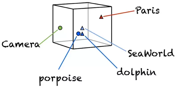
Сегодня мы говорим про слова и стоит обсудить, как делать такое сопоставление вектора слову.
Вернемся к предмету: вот у нас есть слова и есть компьютер, который должен с этими словами как-то работать. Вопрос — как компьютер будет работать со словами? Ведь компьютер не умеет читать, и вообще устроен сильно иначе, чем человек. Самая первая идея, приходящая в голову — просто закодировать слова цифрами по порядку следования в словаре. Идея очень продуктивна в своей простоте — натуральный ряд бесконечен и можно перенумеровать все слова, не опасаясь проблем. (На секунду забудем про ограничения типов, тем более, в 64-битное слово можно запихнуть числа от 0 до 2^64 — 1, что существенно больше количества всех слов всех известных языков.)
Но у этой идеи есть и существенный недостаток: слова в словаре следуют в алфавитном порядке, и при добавлении слова нужно перенумеровывать заново большую часть слов. Но даже это не является настолько важным, а важно то, буквенное написание слова никак не связано с его смыслом (эту гипотезу еще в конце XIX века высказал известный лингвист Фердинанд де Соссюр). В самом деле слова “петух”, “курица” и “цыпленок” имеют очень мало общего между собой и стоят в словаре далеко друг от друга, хотя очевидно обозначают самца, самку и детеныша одного вида птицы. То есть мы можем выделить два вида близости слов: лексический и семантический. Как мы видим на примере с курицей, эти близости не обязательно совпадают. Можно для наглядности привести обратный пример лексически близких, но семантически далеких слов — «зола» и «золото». (Если вы никогда не задумывались, то имя Золушка происходит именно от первого.)
Чтобы получить возможность представить семантическую близость, было предложено использовать embedding, то есть сопоставить слову некий вектор, отображающий его значение в “пространстве смыслов”.
Какой самый простой способ получить вектор из слова? Кажется, что естественно будет взять вектор длины нашего словаря и поставить только одну единицу в позиции, соответствующей номеру слова в словаре. Этот подход называется one-hot encoding (OHE). OHE все еще не обладает свойствами семантической близости:

Значит нам нужно найти другой способ преобразования слов в вектора, но OHE нам еще пригодится.
Отойдем немного назад — значение одного слова нам может быть и не так важно, т.к. речь (и устная, и письменная) состоит из наборов слов, которые мы называем текстами. Так что если мы захотим как-то представить тексты, то мы возьмем OHE-вектор каждого слова в тексте и сложим вместе. Т.е. на выходе получим просто подсчет количества различных слов в тексте в одном векторе. Такой подход называется “мешок слов” (bag of words, BoW), потому что мы теряем всю информацию о взаимном расположении слов внутри текста.
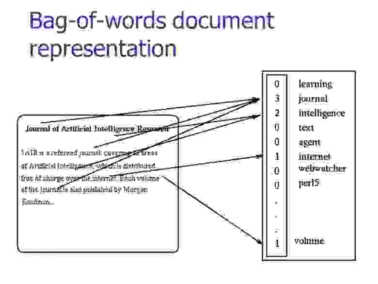
Но несмотря на потерю этой информации так тексты уже можно сравнивать. Например, с помощью косинусной меры.
Мы можем пойти дальше и представить наш корпус (набор текстов) в виде матрицы “слово-документ” (term-document). Стоит отметить, что в области информационного поиска (information retrieval) эта матрица носит название «обратного индекса» (inverted index), в том смысле, что обычный/прямой индекс выглядит как «документ-слово» и очень неудобен для быстрого поиска. Но это опять же выходит за рамки нашей статьи.
Эта матрица приводит нас к тематическим моделям, где матрицу “слово-документ” пытаются представить в виде произведения двух матриц “слово-тема” и “тема-документ”. В самом простом случае мы возьмем матрицу и с помощью SVD-разложения получим представление слов через темы и документов через темы:

Здесь  — слова,
  — документы. Но это уже будет предметом другой статьи, а сейчас мы вернемся к нашей главной теме — векторному представлению слов.
Пусть у нас есть такой корпус:
s = ['Mars has an athmosphere', "Saturn 's moon Titan has its own athmosphere",
     'Mars has two moons', 'Saturn has many moons', 'Io has cryo-vulcanoes']
С помощью SVD-преобразования, выделим только первые две компоненты, и нарисуем:
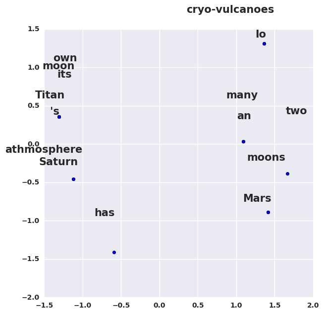
Что интересного на этой картинке? То, что Титан и Ио — далеко друг от друга, хотя они оба являются спутниками Сатурна, но в нашем корпусе про это ничего нет. Слова «атмосфера» и «Сатурн» очень близко друг другу, хотя не являются синонимами. В то же время «два» и «много» стоят рядом, что логично. Но общий смысл этого примера в том, что результаты, которые вы получите очень сильно зависят от корпуса, с которым вы работаете. Весь код для получения картинки выше можно посмотреть здесь.
Логика повествования выводит на следующую модификацию матрицы term-document — формулу TF-IDF. Эта аббревиатура означает «term frequency — inverse document frequency».

Давайте попробуем разобраться, что это такое. Итак, TF — это частота слова  в тексте
  , здесь нет ничего сложного. А вот IDF — существенно более интересная вещь: это логарифм обратной частоты распространенности слова в корпусе
  . Распространенностью называется отношение числа текстов, в которых встретилось искомое слово, к общему числу текстов в корпусе. С помощью TF-IDF тексты также можно сравнивать, и делать это можно с меньшей опаской, чем при использовании обычных частот.
Новая эпоха
Описанные выше подходы были (и остаются) хороши для времен (или областей), где количество текстов мало и словарь ограничен, хотя, как мы видели, там тоже есть свои сложности. Но с приходом в нашу жизнь интернета все стало одновременно и сложнее и проще: в доступе появилось великое множество текстов, и эти тексты с изменяющимся и расширяющимся словарем. С этим надо было что-то делать, а ранее известные модели не могли справиться с таким объемом текстов. Количество слов в английском языке очень грубо составляет миллион — матрица совместных встречаемостей только пар слов будет 10^6 x 10^6. Такая матрица даже сейчас не очень лезет в память компьютеров, а, скажем, 10 лет назад про такое можно было не мечтать. Конечно, были придуманы множество способов, упрощающих или распараллеливающих обработку таких матриц, но все это были паллиативные методы.
И тогда, как это часто бывает, был предложен выход по принципу “тот, кто нам мешает, тот нам поможет!” А именно, в 2013 году тогда мало кому известный чешский аспирант Томаш Миколов предложил свой подход к word embedding, который он назвал word2vec. Его подход основан на другой важной гипотезе, которую в науке принято называть гипотезой локальности — “слова, которые встречаются в одинаковых окружениях, имеют близкие значения”. Близость в данном случае понимается очень широко, как то, что рядом могут стоять только сочетающиеся слова. Например, для нас привычно словосочетание «заводной будильник». А сказать “заводной апельсин” мы не можем* — эти слова не сочетаются.
Основываясь на этой гипотезе Томаш Миколов предложил новый подход, который не страдал от больших объемов информации, а наоборот выигрывал [1].

Модель, предложенная Миколовым очень проста (и потому так хороша) — мы будем предсказывать вероятность слова по его окружению (контексту). То есть мы будем учить такие вектора слов, чтобы вероятность, присваиваемая моделью слову была близка к вероятности встретить это слово в этом окружении в реальном тексте.

Здесь  — вектор целевого слова,
  — это некоторый вектор контекста, вычисленный (например, путем усреднения) из векторов окружающих нужное слово других слов. А
  — это функция, которая двум векторам сопоставляет одно число. Например, это может быть упоминавшееся выше косинусное расстояние.
Приведенная формула называется softmax, то есть “мягкий максимум”, мягкий — в смысле дифференцируемый. Это нужно для того, чтобы наша модель могла обучиться с помощью backpropagation, то есть процесса обратного распространения ошибки.
Процесс тренировки устроен следующим образом: мы берем последовательно (2k+1) слов, слово в центре является тем словом, которое должно быть предсказано. А окружающие слова являются контекстом длины по k с каждой стороны. Каждому слову в нашей модели сопоставлен уникальный вектор, который мы меняем в процессе обучения нашей модели.
В целом, этот подход называется CBOW — continuous bag of words, continuous потому, что мы скармливаем нашей модели последовательно наборы слов из текста, a BoW потому что порядок слов в контексте не важен.
Также Миколовым сразу был предложен другой подход — прямо противоположный CBOW, который он назвал skip-gram, то есть “словосочетание с пропуском”. Мы пытаемся из данного нам слова угадать его контекст (точнее вектор контекста). В остальном модель не претерпевает изменений.
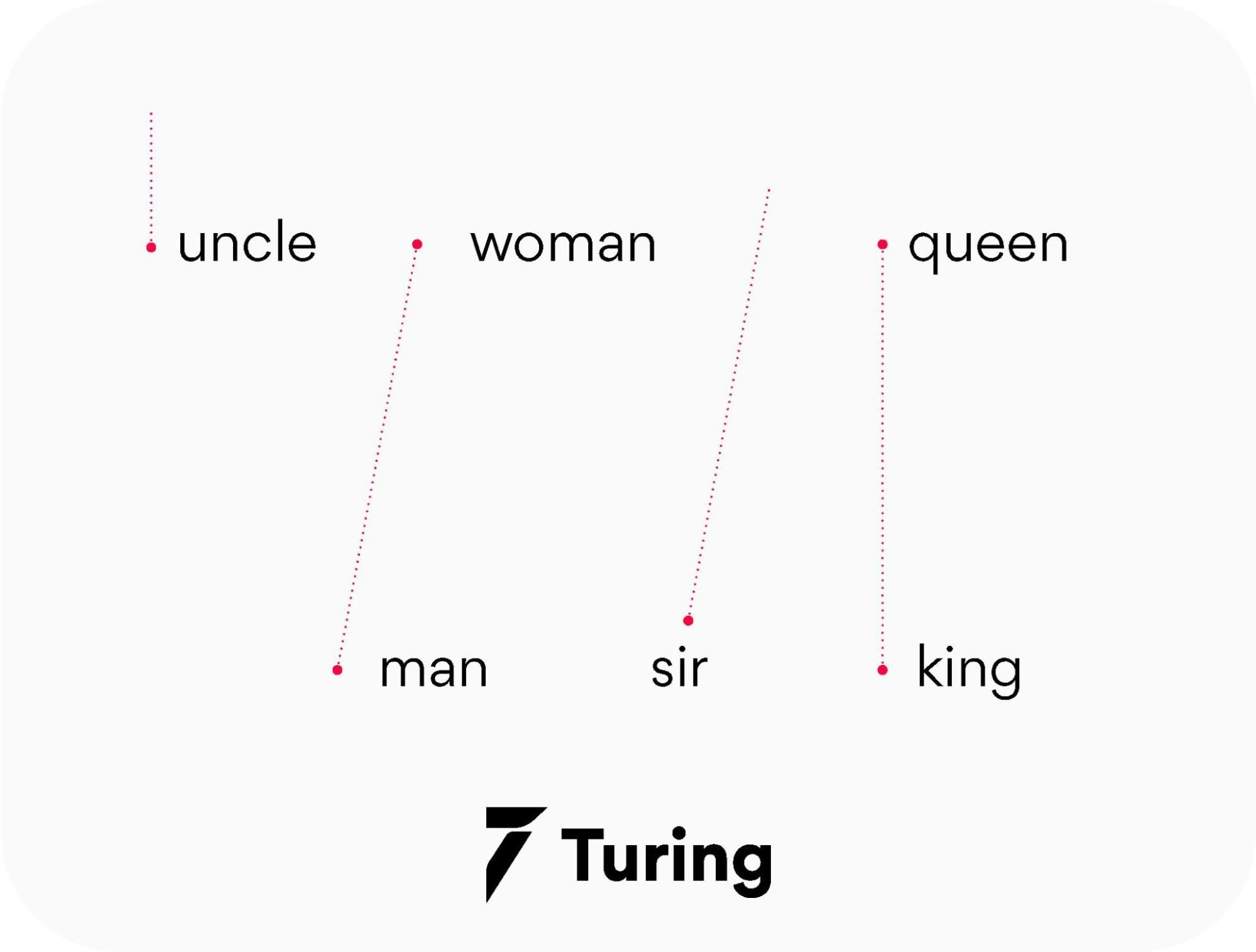
Что стоит отметить: хотя в модель не заложено явно никакой семантики, а только статистические свойства корпусов текстов, оказывается, что натренированная модель word2vec может улавливать некоторые семантические свойства слов. Классический пример из работы автора:
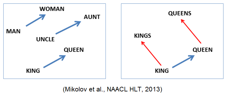
Слово «мужчина» относится к слову «женщина» так же, как слово «дядя» к слову «тётя», что для нас совершенно естественно и понятно, но в других моделям добиться такого же соотношения векторов можно только с помощью специальных ухищрений. Здесь же — это происходит естественно из самого корпуса текстов. Кстати, помимо семантических связей, улавливаются и синтаксические, справа показано соотношение единственного и множественного числа.
Более сложные вещи
На самом деле, за прошедшее время были предложены улучшения ставшей уже также классической модели Word2Vec. Два самых распространенных будут описаны ниже. Но этот раздел может быть пропущен без ущерба для понимания статьи в целом, если покажется слишком сложным.
Negative Sampling
В стандартной модели CBoW, рассмотренной выше, мы предсказываем вероятности слов и оптимизируем их. Функцией для оптимизации (минимизации в нашем случае) служит дивергенция Кульбака-Лейблера:

Здесь  — распределение вероятностей слов, которое мы берем из корпуса,
  — распределение, которое порождает наша модель. Дивергенция — это буквально «расхождение», насколько одно распределение не похоже на другое. Т.к. наши распределения на словах, т.е. являются дискретными, мы можем заменить в этой формуле интеграл на сумму:

Оказалось так, что оптимизировать эту формулу достаточно сложно. Прежде всего из-за того, что рассчитывается с помощью softmax по всему словарю. (Как мы помним, в английском сейчас порядка миллиона слов.) Здесь стоит отметить, что многие слова вместе не встречаются, как мы уже отмечали выше, поэтому большая часть вычислений в softmax является избыточной. Был предложен элегантный обходной путь, который получил название Negative Sampling. Суть этого подхода заключается в том, что мы максимизируем вероятность встречи для нужного слова в типичном контексте (том, который часто встречается в нашем корпусе) и одновременно минимизируем вероятность встречи в нетипичном контексте (том, который редко или вообще не встречается). Формулой мысль выше записывается так:

Здесь  — точно такой же, что и в оригинальной формуле, а вот остальное несколько отличается. Прежде всего стоит обратить внимание на то, что формуле теперь состоит из двух частей: позитивной () и негативной (
 ). Позитивная часть отвечает за типичные контексты, и
  здесь — это распределение совместной встречаемости слова и остальных слов корпуса. Негативная часть — это, пожалуй, самое интересное — это набор слов, которые с нашим целевым словом встречаются редко. Этот набор порождается из распределения
  , которое на практике берется как равномерное по всем словам словаря корпуса. Было показано, что такая функция приводит при своей оптимизации к результату, аналогичному стандартному softmax [2].
Hierarchical SoftMax
Также люди зашли и с другой стороны — можно не менять исходную формулу, а попробовать посчитать сам softmax более эффективно. Например, используя бинарное дерево [3]. По всем словам в словаре строится дерево Хаффмана. В полученном дереве  слов располагаются на листьях дерева.
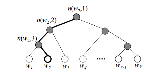
На рисунке изображен пример такого бинарного дерева. Жирным выделен путь от корня до слова  . Длину пути обозначим
  , а
, а  -ую вершину на пути к слову обозначим через
  . Можно доказать, что внутренних вершин (не листьев)
  .
.
С помощью иерархического softmax вектора  предсказывается для
  внутренних вершин. А вероятность того, что слово будет выходным словом (в зависимости от того, что мы предсказываем: слово из контекста или заданное слово по контексту) вычисляется по формуле:
![$p(w=w_o)=prodlimits_{j=1}^{L(w)-1}sigma([n(w,j+1)=lch(n(w,j))] v_{n(w,j)}^T u)$](https://habrastorage.org/getpro/habr/formulas/018/e83/e8f/018e83e8fb17212f7b2c6a6be6d09635.svg)
где  — функция softmax;
 ![$[true]=1,[false]=-1$](https://habrastorage.org/getpro/habr/formulas/870/680/f3e/870680f3ef96594c5444eaeca1440677.svg) ;
;  — левый сын вершины
  ;
;  , если используется метод skip-gram,
  , то есть, усредненный вектор контекста, если используется CBOW.
Формулу можно интуитивно понять, представив, что на каждом шаге мы можем пойти налево или направо с вероятностями:


Затем на каждом шаге вероятности перемножаются ( шагов) и получается искомая формула.
При использовании простого softmax для подсчета вероятности слова, приходилось вычислять нормирующую сумму по всем словам из словаря, требовалось  операций. Теперь же вероятность слова можно вычислить при помощи последовательных вычислений, которые требуют
  .
.
Другие модели
Помимо word2vec были, само собой, предложены и другие модели word embedding. Стоит отметить модель, предложенную лабораторией компьютерной лингвистики Стенфордского университета, под названием Global Vectors (GloVe), сочетающую в себе черты SVD разложения и word2vec [4].
Также надо упомянуть о том, что т.к. изначально все описанные модели были предложены для английского языка, то там не так остро стоит проблема словоизменения, характерная для синтетических языков (это — лингвистический термин), вроде русского. Везде выше по тексту неявно предполагалось, что мы либо считаем разные формы одного слова разными словами — и тогда надеяться, что нашего корпуса будет достаточно модели, чтобы выучить их синтаксическую близость, либо используем механизмы стеммирования или лемматизации. Стеммирование — это обрезание окончания слова, оставление только основы (например, “красного яблока” превратится в “красн яблок”). А лемматизация — замена слова его начальной формой (например, “мы бежим” превратится в “я бежать”). Но мы можем и не терять эту информацию, а использовать ее — закодировав OHE в новый вектор, и сконкатинировать его с вектором для основы или леммы.
Еще стоит сказать, что то, с чем мы начинали — буквенное представление слова — тоже не кануло в Лету: предложены модели по использованию буквенного представления слова для word embedding [5].
Практическое применение
Мы поговорили о теории, пришло время посмотреть, к чему все вышеописанное применимо на практике. Ведь любая самая красивая теория без практического применения — не более чем игра ума. Рассмотрим применение Word2Vec в двух задачах:
1) Задача классификации, необходимо по последовательности посещенных сайтов определять пользователя;
2) Задача регрессии, необходимо по тексту статьи определить ее рейтинг на Хабрахабре.
Классификация
# загрузим библиотеки и установим опции
from __future__ import division, print_function
# отключим всякие предупреждения Anaconda
import warnings
warnings.filterwarnings('ignore')
#%matplotlib inline
import numpy as np
import pandas as pd
from sklearn.metrics import roc_auc_score
Cкачать данные для первой задачи можно со страницы соревнования «Catch Me If You Can»
# загрузим обучающую и тестовую выборки
train_df = pd.read_csv('data/train_sessions.csv')#,index_col='session_id')
test_df = pd.read_csv('data/test_sessions.csv')#, index_col='session_id')

# приведем колонки time1, ..., time10 к временному формату
times = ['time%s' % i for i in range(1, 11)]
train_df[times] = train_df[times].apply(pd.to_datetime)
test_df[times] = test_df[times].apply(pd.to_datetime)

# отсортируем данные по времени
train_df = train_df.sort_values(by='time1')

# посмотрим на заголовок обучающей выборки
train_df.head()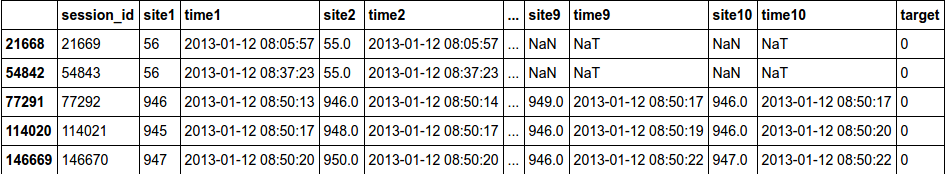
sites = ['site%s' % i for i in range(1, 11)]
#заменим nan на 0
train_df[sites] = train_df[sites].fillna(0).astype('int').astype('str')
test_df[sites] = test_df[sites].fillna(0).astype('int').astype('str')
#создадим тексты необходимые для обучения word2vec
train_df['list'] = train_df['site1']
test_df['list'] = test_df['site1']
for s in sites[1:]:
    train_df['list'] = train_df['list']+","+train_df[s]
    test_df['list'] = test_df['list']+","+test_df[s]
train_df['list_w'] = train_df['list'].apply(lambda x: x.split(','))
test_df['list_w'] = test_df['list'].apply(lambda x: x.split(','))
#В нашем случае предложение это набор сайтов, которые посещал пользователь
#нам необязательно переводить цифры в названия сайтов, т.к. алгоритм будем выявлять взаимосвязь их друг с другом.
train_df['list_w'][10]['229', '1500', '33', '1500', '391', '35', '29', '2276', '40305', '23']# подключим word2vec
from gensim.models import word2vec#объединим обучающую и тестовую выборки и обучим нашу модель на всех данных
#с размером окна в 6=3*2 (длина предложения 10 слов) и итоговыми векторами размерности 300, параметр workers отвечает за количество ядер
test_df['target'] = -1
data = pd.concat([train_df,test_df], axis=0)
model = word2vec.Word2Vec(data['list_w'], size=300, window=3, workers=4)
#создадим словарь со словами и соответсвующими им векторами
w2v = dict(zip(model.wv.index2word, model.wv.syn0))Т.к. сейчас мы каждому слову сопоставили вектор, то нужно решить, что сопоставить целому предложению из слов.
Один из возможных вариантов это просто усреднить все слова в предложении и получить некоторый смысл всего предложения (если слова нет в тексте, то берем нулевой вектор).
class mean_vectorizer(object):
    def __init__(self, word2vec):
        self.word2vec = word2vec
        self.dim = len(next(iter(w2v.values())))

    def fit(self, X):
        return self

    def transform(self, X):
        return np.array([
            np.mean([self.word2vec[w] for w in words if w in self.word2vec]
                    or [np.zeros(self.dim)], axis=0)
            for words in X
        ])
data_mean=mean_vectorizer(w2v).fit(train_df['list_w']).transform(train_df['list_w'])
data_mean.shape(253561, 300)Т.к. мы получили distributed representation, то никакое число по отдельности ничего не значит, а значит лучше всего покажут себя линейные алгоритмы. Попробуем нейронные сети, LogisticRegression и проверим нелинейный метод XGBoost.
# Воспользуемся валидацией
def split(train,y,ratio):
    idx = round(train.shape[0] * ratio)
    return train[:idx, :], train[idx:, :], y[:idx], y[idx:]
y = train_df['target']
Xtr, Xval, ytr, yval = split(data_mean, y,0.8)
Xtr.shape,Xval.shape,ytr.mean(),yval.mean()
((202849, 300), (50712, 300), 0.009726446765820882, 0.006389020350212968)# подключим библиотеки keras
from keras.models import Sequential, Model
from keras.layers import Dense, Dropout, Activation, Input
from keras.preprocessing.text import Tokenizer
from keras import regularizers# опишем нейронную сеть
model = Sequential()
model.add(Dense(128, input_dim=(Xtr.shape[1])))
model.add(Activation('relu'))
model.add(Dropout(0.5))
model.add(Dense(1))
model.add(Activation('sigmoid'))
model.compile(loss='binary_crossentropy',
optimizer='adam',
metrics=['binary_accuracy'])history = model.fit(Xtr, ytr,
batch_size=128,
epochs=10,
validation_data=(Xval, yval),
class_weight='auto',
verbose=0)classes = model.predict(Xval, batch_size=128)
roc_auc_score(yval, classes)0.91892341356995644Получили неплохой результат. Значит Word2Vec смог выявить зависимости между сессиями.
Посмотрим, что произойдет с алгоритмом XGBoost.
import xgboost as xgbdtr = xgb.DMatrix(Xtr, label= ytr,missing = np.nan)
dval = xgb.DMatrix(Xval, label= yval,missing = np.nan)
watchlist = [(dtr, 'train'), (dval, 'eval')]
history = dict()params = {
'max_depth': 26,
'eta': 0.025,
'nthread': 4,
'gamma' : 1,
'alpha' : 1,
'subsample': 0.85,
'eval_metric': ['auc'],
'objective': 'binary:logistic',
'colsample_bytree': 0.9,
'min_child_weight': 100,
'scale_pos_weight':(1)/y.mean(),
'seed':7
}model_new = xgb.train(params, dtr, num_boost_round=200, evals=watchlist, evals_result=history, verbose_eval=20)Обучение
[0] train-auc:0.954886 eval-auc:0.85383
[20] train-auc:0.989848 eval-auc:0.910808
[40] train-auc:0.992086 eval-auc:0.916371
[60] train-auc:0.993658 eval-auc:0.917753
[80] train-auc:0.994874 eval-auc:0.918254
[100] train-auc:0.995743 eval-auc:0.917947
[120] train-auc:0.996396 eval-auc:0.917735
[140] train-auc:0.996964 eval-auc:0.918503
[160] train-auc:0.997368 eval-auc:0.919341
[180] train-auc:0.997682 eval-auc:0.920183Видим, что алгоритм сильно подстраивается под обучающую выборку, поэтому возможно наше предположение о необходимости использовать линейные алгоритмы подтверждено.
Посмотрим, что покажет обычный LogisticRegression.
from sklearn.linear_model import LogisticRegression
def get_auc_lr_valid(X, y, C=1, seed=7, ratio = 0.8):
# разделим выборку на обучающую и валидационную
idx = round(X.shape[0] * ratio)
# обучение классификатора
lr = LogisticRegression(C=C, random_state=seed, n_jobs=-1).fit(X[:idx], y[:idx])
# прогноз для валидационной выборки
y_pred = lr.predict_proba(X[idx:, :])[:, 1]
# считаем качество
score = roc_auc_score(y[idx:], y_pred)
return scoreget_auc_lr_valid(data_mean, y, C=1, seed=7, ratio = 0.8)0.90037148150108237Попробуем улучшить результаты.
Теперь вместо обычного среднего, чтобы учесть частоту с которой слово встречается в тексте, возьмем взвешенное среднее. В качестве весов возьмем IDF. Учёт IDF уменьшает вес широко употребительных слов и увеличивает вес более редких слов, которые могут достаточно точно указать на то, к какому классу относится текст. В нашем случае, кому принадлежит последовательность посещенных сайтов.
#пропишем класс выполняющий tfidf преобразование.
from sklearn.feature_extraction.text import TfidfVectorizer
from collections import defaultdict
class tfidf_vectorizer(object):
def __init__(self, word2vec):
self.word2vec = word2vec
self.word2weight = None
self.dim = len(next(iter(w2v.values())))
def fit(self, X):
tfidf = TfidfVectorizer(analyzer=lambda x: x)
tfidf.fit(X)
max_idf = max(tfidf.idf_)
self.word2weight = defaultdict(
lambda: max_idf,
[(w, tfidf.idf_[i]) for w, i in tfidf.vocabulary_.items()])
return self
def transform(self, X):
return np.array([
np.mean([self.word2vec[w] * self.word2weight[w]
for w in words if w in self.word2vec] or
[np.zeros(self.dim)], axis=0)
for words in X
])data_mean = tfidf_vectorizer(w2v).fit(train_df['list_w']).transform(train_df['list_w'])Проверим изменилось ли качество LogisticRegression.
get_auc_lr_valid(data_mean, y, C=1, seed=7, ratio = 0.8)0.90738924587178804видим прирост на 0.07, значит скорее всего взвешенное среднее помогает лучше отобразить смысл всего предложения через word2vec.
Предсказание популярности
Попробуем Word2Vec уже в текстовой задаче — предсказании популярности статьи на Хабрхабре.
Испробуем силы алгоритма непосредственно на текстовых данных статей Хабра. Мы преобразовали данные в csv таблицы. Скачать их вы можете здесь: train, test.
Xtrain = pd.read_csv('data/train_content.csv')
Xtest = pd.read_csv('data/test_content.csv')
print(Xtrain.shape,Xtest.shape)
Xtrain.head()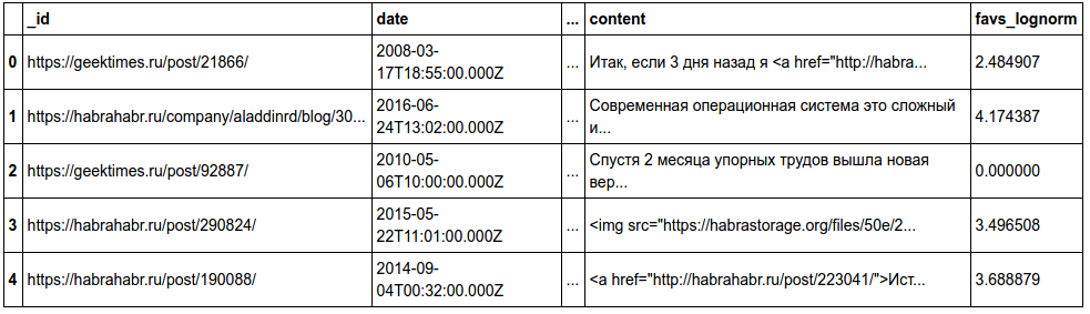
Пример текста
‘Доброго хабрадня!
rn
rnПерейду сразу к сути. С недавнего времени на меня возложилась задача развития контекстной сети текстовых объявлений. Задача возможно кому-то покажется простой, но есть несколько нюансов. Страна маленькая, 90% интернет-пользователей сконцентрировано в одном городе. С одной стороны легко охватить, с другой стороны некуда развиваться.
rn
rnТак как развитие интернет-проектов у нас слабое, и недоверие клиентов к местным проектам преобладает, то привлечь рекламодателей тяжело. Но самое страшное это привлечь площадки, которые знают и Бегун и AdSense, но абсолютно не знают нас. В целом проблема такая: площадки не регистрируются, потому что нет рекламодателей с деньгами, а рекламодатели не дают объявления, потому что список площадок слаб.
rn
rnКак выходят из такого положения Хабраспециалисты?’
Будем обучать модель на всем содержании статьи. Для этого совершим некоторые преобразования над текстом.
Напишем функцию, которая будет преобразовывать тестовую статью в лист из слов необходимый для обучения Word2Vec.
Функция получает строку, в которой содержится весь текстовый документ.
1) Сначала функция будет удалять все символы кроме букв верхнего и нижнего регистра;
2) Затем преобразовывает слова к нижнему регистру;
3) После чего удаляет стоп слова из текста, т.к. они не несут никакой информации о содержании;
4) Лемматизация, процесс приведения словоформы к лемме — её нормальной (словарной) форме.
Функция возвращает лист из слов.
# подключим необходимые библиотеки
from sklearn.metrics import mean_squared_error
import re
from nltk.corpus import stopwords
import pymorphy2
morph = pymorphy2.MorphAnalyzer()
stops = set(stopwords.words("english")) | set(stopwords.words("russian"))
def review_to_wordlist(review):
#1)
review_text = re.sub("[^а-яА-Яa-zA-Z]"," ", review)
#2)
words = review_text.lower().split()
#3)
words = [w for w in words if not w in stops]
#4)
words = [morph.parse(w)[0].normal_form for w in words ]
return(words)
Лемматизация занимает много времени, поэтому ее можно убрать в целях более быстрых подсчетов.
# Преобразуем время
Xtrain['date'] = Xtrain['date'].apply(pd.to_datetime)
Xtrain['year'] = Xtrain['date'].apply(lambda x: x.year)
Xtrain['month'] = Xtrain['date'].apply(lambda x: x.month)Будем обучаться на 2015 году, а валидироваться по первым 4 месяцам 2016, т.к. в нашей тестовой выборке представлены данные за первые 4 месяца 2017 года. Более правдивую валидацию можно сделать, идя по годам, увеличивая нашу обучающую выборку и смотря качество на первых четырех месяцах следующего года
Xtr = Xtrain[Xtrain['year']==2015]
Xval = Xtrain[(Xtrain['year']==2016)& (Xtrain['month']<=4)]
ytr = Xtr['favs_lognorm']
yval = Xval['favs_lognorm']
Xtr.shape,Xval.shape,ytr.mean(),yval.mean()((23425, 15), (7556, 15), 3.4046228249071526, 3.304679829935242)data = pd.concat([Xtr,Xval],axis = 0,ignore_index = True)#у нас есть nan, поэтому преобразуем их к строке
data['content_clear'] = data['content'].apply(str)%%time
data['content_clear'] = data['content_clear'].apply(review_to_wordlist)model = word2vec.Word2Vec(data['content_clear'], size=300, window=10, workers=4)
w2v = dict(zip(model.wv.index2word, model.wv.syn0))Посмотрим чему выучилась модель:
model.wv.most_similar(positive=['open', 'data','science','best'])Результат
[(‘massive’, 0.6958945393562317),
(‘mining’, 0.6796239018440247),
(‘scientist’, 0.6742461919784546),
(‘visualization’, 0.6403135061264038),
(‘centers’, 0.6386666297912598),
(‘big’, 0.6237790584564209),
(‘engineering’, 0.6209672689437866),
(‘structures’, 0.609510600566864),
(‘knowledge’, 0.6094595193862915),
(‘scientists’, 0.6050446629524231)]
Модель обучилась достаточно неплохо, посмотрим на результаты алгоритмов:
data_mean = mean_vectorizer(w2v).fit(data['content_clear']).transform(data['content_clear'])
data_mean.shapedef split(train,y,ratio):
idx = ratio
return train[:idx, :], train[idx:, :], y[:idx], y[idx:]
y = data['favs_lognorm']
Xtr, Xval, ytr, yval = split(data_mean, y,23425)
Xtr.shape,Xval.shape,ytr.mean(),yval.mean()((23425, 300), (7556, 300), 3.4046228249071526, 3.304679829935242)from sklearn.linear_model import Ridge
from sklearn.metrics import mean_squared_error
model = Ridge(alpha = 1,random_state=7)
model.fit(Xtr, ytr)
train_preds = model.predict(Xtr)
valid_preds = model.predict(Xval)
ymed = np.ones(len(valid_preds))*ytr.median()
print('Ошибка на трейне',mean_squared_error(ytr, train_preds))
print('Ошибка на валидации',mean_squared_error(yval, valid_preds))
print('Ошибка на валидации предсказываем медиану',mean_squared_error(yval, ymed))Ошибка на трейне 0.734248488422
Ошибка на валидации 0.665592676973
Ошибка на валидации предсказываем медиану 1.44601638512data_mean_tfidf = tfidf_vectorizer(w2v).fit(data['content_clear']).transform(data['content_clear'])y = data['favs_lognorm']
Xtr, Xval, ytr, yval = split(data_mean_tfidf, y,23425)
Xtr.shape,Xval.shape,ytr.mean(),yval.mean()((23425, 300), (7556, 300), 3.4046228249071526, 3.304679829935242)model = Ridge(alpha = 1,random_state=7)
model.fit(Xtr, ytr)
train_preds = model.predict(Xtr)
valid_preds = model.predict(Xval)
ymed = np.ones(len(valid_preds))*ytr.median()
print('Ошибка на трейне',mean_squared_error(ytr, train_preds))
print('Ошибка на валидации',mean_squared_error(yval, valid_preds))
print('Ошибка на валидации предсказываем медиану',mean_squared_error(yval, ymed))Ошибка на трейне 0.743623730976
Ошибка на валидации 0.675584372744
Ошибка на валидации предсказываем медиану 1.44601638512Попробуем нейронные сети.
# подключим библиотеки keras
from keras.models import Sequential, Model
from keras.layers import Dense, Dropout, Activation, Input
from keras.preprocessing.text import Tokenizer
from keras import regularizers
from keras.wrappers.scikit_learn import KerasRegressor# Опишем нашу сеть.
def baseline_model():
model = Sequential()
model.add(Dense(128, input_dim=Xtr.shape[1], kernel_initializer='normal', activation='relu'))
model.add(Dropout(0.2))
model.add(Dense(64, activation='relu'))
model.add(Dropout(0.5))
model.add(Dense(1, kernel_initializer='normal'))
model.compile(loss='mean_squared_error', optimizer='adam')
return model
estimator = KerasRegressor(build_fn=baseline_model,epochs=20, nb_epoch=20, batch_size=64,validation_data=(Xval, yval), verbose=2)estimator.fit(Xtr, ytr)Обучение
Train on 23425 samples, validate on 7556 samples
Epoch 1/20
1s — loss: 1.7292 — val_loss: 0.7336
Epoch 2/20
0s — loss: 1.2382 — val_loss: 0.6738
Epoch 3/20
0s — loss: 1.1379 — val_loss: 0.6916
Epoch 4/20
0s — loss: 1.0785 — val_loss: 0.6963
Epoch 5/20
0s — loss: 1.0362 — val_loss: 0.6256
Epoch 6/20
0s — loss: 0.9858 — val_loss: 0.6393
Epoch 7/20
0s — loss: 0.9508 — val_loss: 0.6424
Epoch 8/20
0s — loss: 0.9066 — val_loss: 0.6231
Epoch 9/20
0s — loss: 0.8819 — val_loss: 0.6207
Epoch 10/20
0s — loss: 0.8634 — val_loss: 0.5993
Epoch 11/20
1s — loss: 0.8401 — val_loss: 0.6093
Epoch 12/20
1s — loss: 0.8152 — val_loss: 0.6006
Epoch 13/20
0s — loss: 0.8005 — val_loss: 0.5931
Epoch 14/20
0s — loss: 0.7736 — val_loss: 0.6245
Epoch 15/20
0s — loss: 0.7599 — val_loss: 0.5978
Epoch 16/20
1s — loss: 0.7407 — val_loss: 0.6593
Epoch 17/20
1s — loss: 0.7339 — val_loss: 0.5906
Epoch 18/20
1s — loss: 0.7256 — val_loss: 0.5878
Epoch 19/20
1s — loss: 0.7117 — val_loss: 0.6123
Epoch 20/20
0s — loss: 0.7069 — val_loss: 0.5948
Получили более хороший результат по сравнению с гребневой регрессией.
Заключение
Word2Vec показал свою пользу на практических задачах анализа текстов, все-таки не зря на текущий момент на практике используется в основном именно он и — гораздо менее популярный — GloVe. Тем не менее, может быть в вашей конкретной задаче, вам пригодятся подходы, которым для эффективной работы не требуются такие объемы данных, как для word2vec.
Код ноутбуков с примерами можно взять здесь. Код практического применения — вот тут.
Пост написан совместно с demonzheg.
Литература
- Tomas Mikolov, Kai Chen, Greg Corrado, and Jeffrey Dean. Efficient estimation
of word representations in vector space. CoRR, abs/1301.3781, - Tomas Mikolov, Ilya Sutskever, Kai Chen, Gregory S. Corrado, and Jeffrey Dean. Distributed representations of words and phrases and their compositionality. In Advances in Neural Information Processing Systems 26: 27th Annual Conference on Neural Information Processing Systems 2013. Proceedings of a meeting held December 5-8, 2013, Lake Tahoe, Nevada, United States, pages 3111–3119, 2013.
- Morin, F., & Bengio, Y. Hierarchical Probabilistic Neural Network Language Model. Aistats, 5, 2005.
- Jeffrey Pennington, Richard Socher, and Christopher D. Manning. GloVe: Global Vectors for Word Representation. 2014.
- Piotr Bojanowski, Edouard Grave, Armand Joulin, and Tomas Mikolov. Enriching word vectors
with subword information. arXiv preprint arXiv:1607.04606, 2016.
* Да, это специальная пасхалка для любителей творчества Энтони Бёрджеса.
Word embedding in NLP is an important term that is used for representing words for text analysis in the form of real-valued vectors. It is an advancement in NLP that has improved the ability of computers to understand text-based content in a better way. It is considered one of the most significant breakthroughs of deep learning for solving challenging natural language processing problems.
In this approach, words and documents are represented in the form of numeric vectors allowing similar words to have similar vector representations. The extracted features are fed into a machine learning model so as to work with text data and preserve the semantic and syntactic information. This information once received in its converted form is used by NLP algorithms that easily digest these learned representations and process textual information.
Due to the perks this technology brings on the table, the popularity of ML NLP is surging making it one of the most chosen fields by the developers.
Now that you have a basic understanding of the topic, let us start from scratch by introducing you to word embeddings, its techniques, and applications.
What is word embedding?
Word embedding or word vector is an approach with which we represent documents and words. It is defined as a numeric vector input that allows words with similar meanings to have the same representation. It can approximate meaning and represent a word in a lower dimensional space. These can be trained much faster than the hand-built models that use graph embeddings like WordNet.
For instance, a word embedding with 50 values holds the capability of representing 50 unique features. Many people choose pre-trained word embedding models like Flair, fastText, SpaCy, and others.
We will discuss it further in the article. Let’s move on to learn it briefly with an example of the same.
The problem
Given a supervised learning task to predict which tweets are about real disasters and which ones are not (classification). Here the independent variable would be the tweets (text) and the target variable would be the binary values (1: Real Disaster, 0: Not real Disaster).
Now, Machine Learning and Deep Learning algorithms only take numeric input. So, how do we convert tweets to their numeric values? We will dive deep into the techniques to solve such problems, but first let’s look at the solution provided by word embedding.
The solution
Word Embeddings in NLP is a technique where individual words are represented as real-valued vectors in a lower-dimensional space and captures inter-word semantics. Each word is represented by a real-valued vector with tens or hundreds of dimensions.
Term frequency-inverse document frequency (TF-IDF)
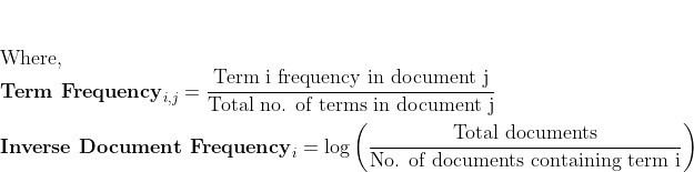
Term frequency-inverse document frequency is the machine learning algorithm that is used for word embedding for text. It comprises two metrics, namely term frequency (TF) and inverse document frequency (IDF).
This algorithm works on a statistical measure of finding word relevance in the text that can be in the form of a single document or various documents that are referred to as corpus.
The term frequency (TF) score measures the frequency of words in a particular document. In simple words, it means that the occurrence of words is counted in the documents.
The inverse document frequency or the IDF score measures the rarity of the words in the text. It is given more importance over the term frequency score because even though the TF score gives more weightage to frequently occurring words, the IDF score focuses on rarely used words in the corpus that may hold significant information.
TF-IDF algorithm finds application in solving simpler natural language processing and machine learning problems for tasks like information retrieval, stop words removal, keyword extraction, and basic text analysis. However, it does not capture the semantic meaning of words efficiently in a sequence.
Now let’s understand it further with an example. We will see how vectorization is done in TF-IDF.

To create TF-IDF vectors, we use Scikit-learn’s TF-IDF Vectorizer. After applying it to the previous 4 sample tweets, we obtain —
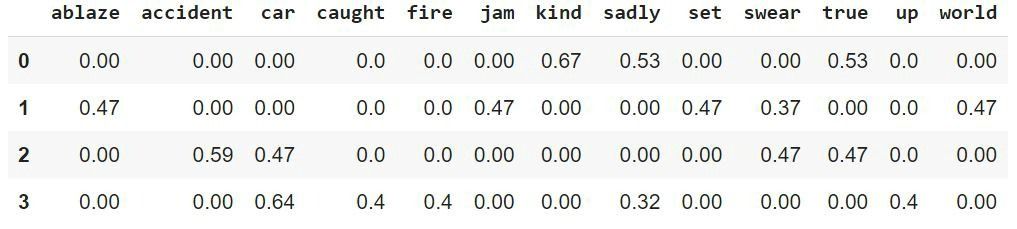
Output of TfidfVectorizer
The rows represent each document, the columns represent the vocabulary, and the values of tf-idf(i,j) are obtained through the above formula. This matrix obtained can be used along with the target variable to train a machine learning/deep learning model.
Let us now discuss two different approaches to word embeddings. We’ll also look at the hands-on part!
Bag of words (BOW)
A bag of words is one of the popular word embedding techniques of text where each value in the vector would represent the count of words in a document/sentence. In other words, it extracts features from the text. We also refer to it as vectorization.
To get you started, here’s how you can proceed to create BOW.
- In the first step, you have to tokenize the text into sentences.
- Next, the sentences tokenized in the first step have further tokenized words.
- Eliminate any stop words or punctuation.
- Then, convert all the words to lowercase.
- Finally, move to create a frequency distribution chart of the words.
We will discuss BOW with proper example in the continuous bag of word selection below.
Word2Vec
Word2Vec method was developed by Google in 2013. Presently, we use this technique for all advanced natural language processing (NLP) problems. It was invented for training word embeddings and is based on a distributional hypothesis.
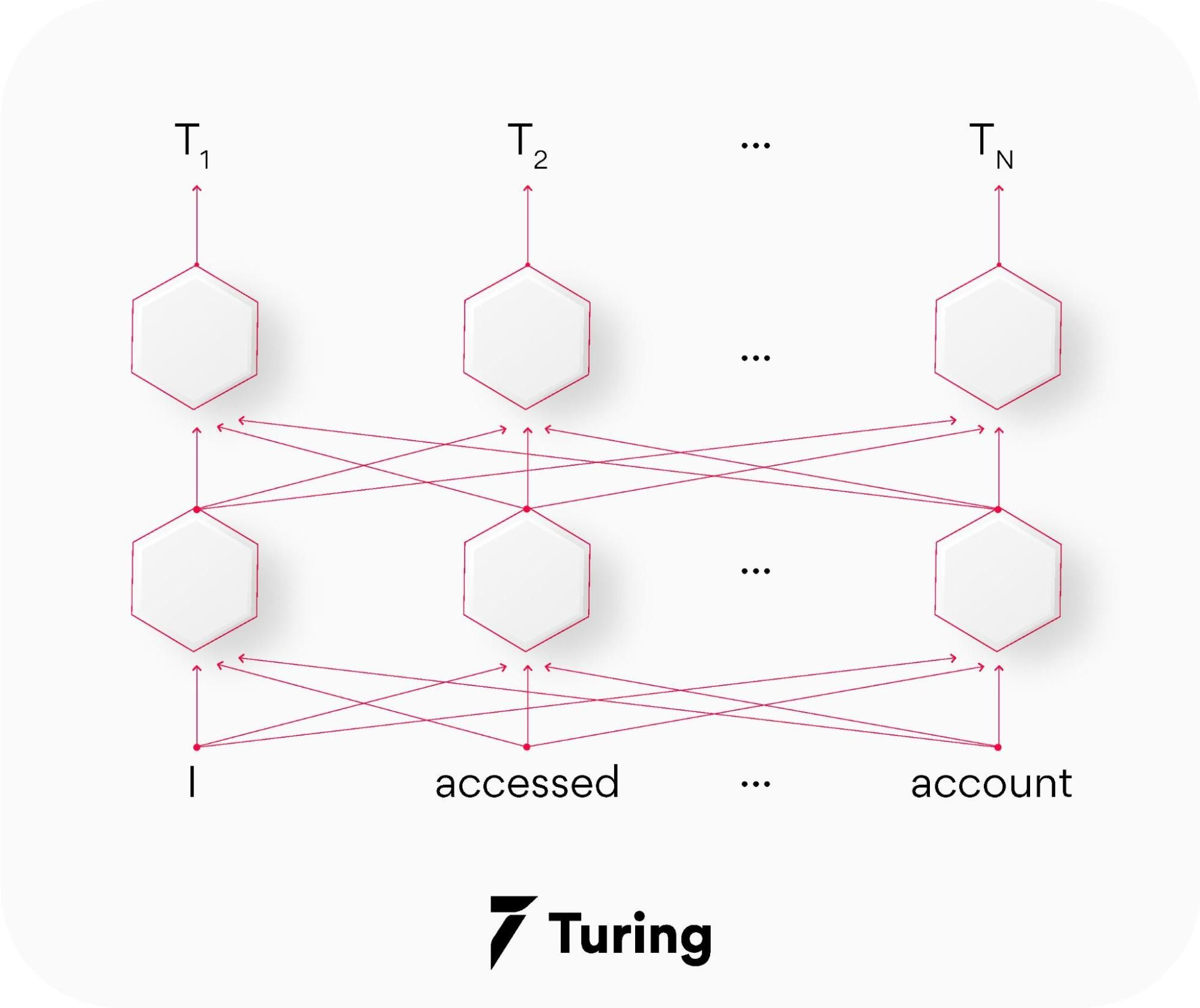
In this hypothesis, it uses skip-grams or a continuous bag of words (CBOW).
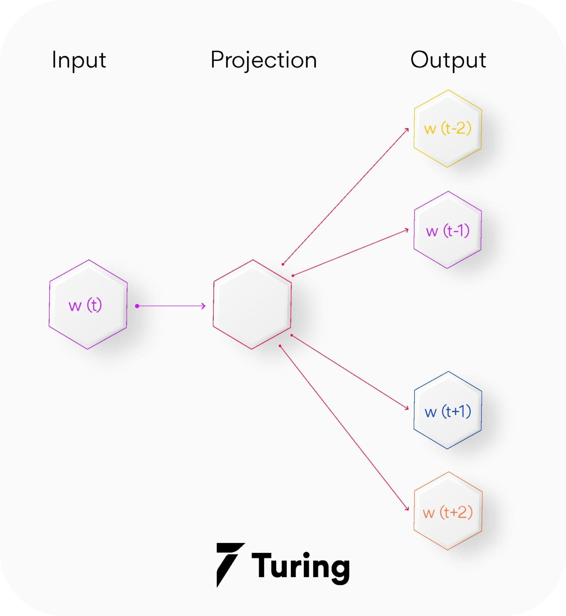
These are basically shallow neural networks that have an input layer, an output layer, and a projection layer. It reconstructs the linguistic context of words by considering both the order of words in history as well as the future.
The method involves iteration over a corpus of text to learn the association between the words. It relies on a hypothesis that the neighboring words in a text have semantic similarities with each other. It assists in mapping semantically similar words to geometrically close embedding vectors.
It uses the cosine similarity metric to measure semantic similarity. Cosine similarity is equal to Cos(angle) where the angle is measured between the vector representation of two words/documents.
-
So if the cosine angle is one, it means that the words are overlapping.
-
And if the cosine angle is a right angle or 90°, It means words hold no contextual similarity and are independent of each other.
To summarize, we can say that this metric assigns similar vector representations to the same boards.
Two variants of Word2Vec
Word2Vec has two neural network-based variants: Continuous Bag of Words (CBOW) and Skip-gram.
1. CBOW — The continuous bag of words variant includes various inputs that are taken by the neural network model. Out of this, it predicts the targeted word that closely relates to the context of different words fed as input. It is fast and a great way to find better numerical representation for frequently occurring words. Let us understand the concept of context and the current word for CBOW.
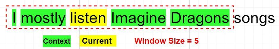
In CBOW, we define a window size. The middle word is the current word and the surrounding words (past and future words) are the context. CBOW utilizes the context to predict the current words. Each word is encoded using One Hot Encoding in the defined vocabulary and sent to the CBOW neural network.
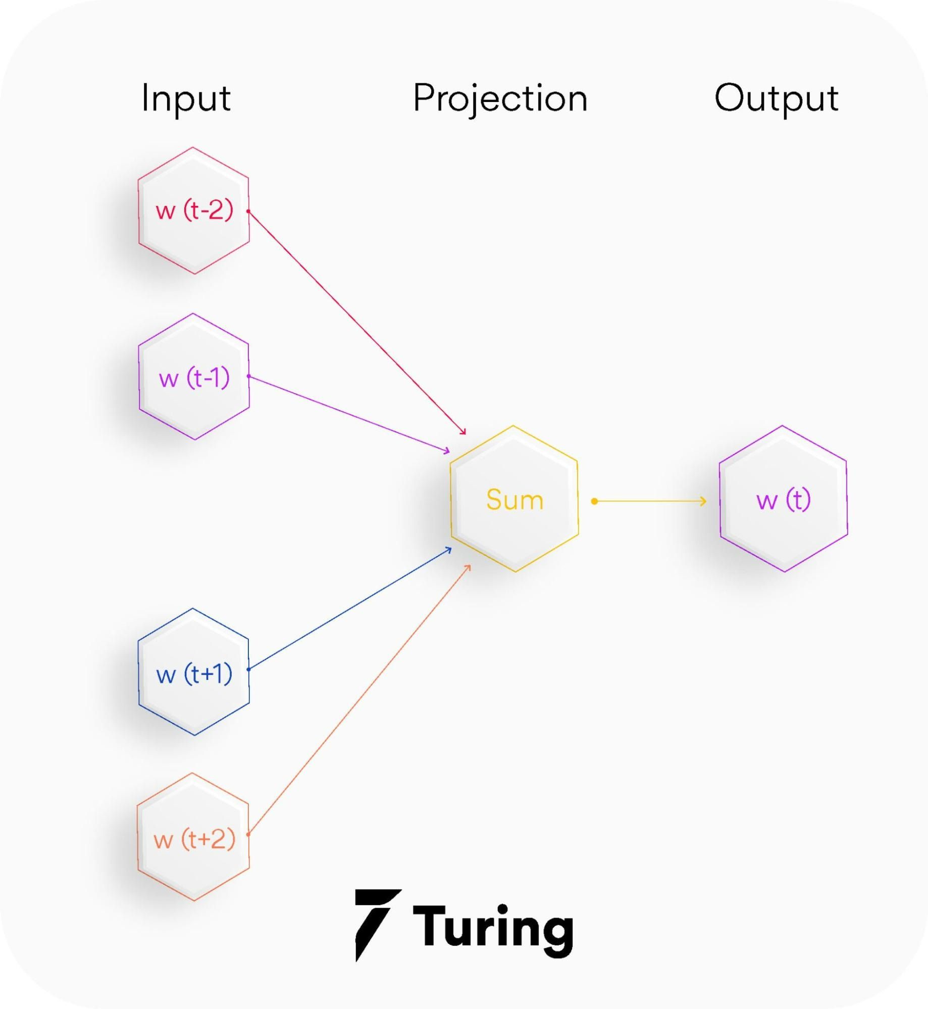
The hidden layer is a standard fully-connected dense layer. The output layer generates probabilities for the target word from the vocabulary.
As we have discussed earlier about the bag of words (BOW) and it being also termed as vectorizer, we will take an example here to clarify it further.
Let’s take a small part of disaster tweets, 4 tweets, to understand how BOW works:-
‘kind true sadly’,
‘swear jam set world ablaze’,
‘swear true car accident’,
‘car sadly car caught up fire’
To create BOW, we use Scikit-learn’s CountVectorizer, which tokenizes a collection of text documents, builds a vocabulary of known words, and encodes new documents using that vocabulary.
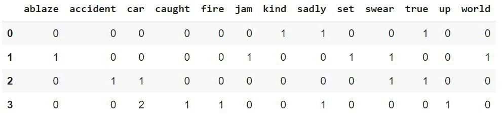
Output of CountVectorizer
Here the rows represent each document (4 in our case), the columns represent the vocabulary (unique words in all the documents) and the values represent the count of the words of the respective rows.
In the same way, we can apply CountVectorizer to the complete training data tweets (11,370 documents) and obtain a matrix that can be used along with the target variable to train a machine learning/deep learning model.
2. Skip-gram — Skip-gram is a slightly different word embedding technique in comparison to CBOW as it does not predict the current word based on the context. Instead, each current word is used as an input to a log-linear classifier along with a continuous projection layer. This way, it predicts words in a certain range before and after the current word.
This variant takes only one word as an input and then predicts the closely related context words. That is the reason it can efficiently represent rare words.
The end goal of Word2Vec (both variants) is to learn the weights of the hidden layer. The hidden consequences will be used as our word embeddings!! Let’s now see the code for creating custom word embeddings using Word2Vec-
Import Libraries
from gensim.models import Word2Vec
import nltk
import re
from nltk.corpus import stopwords
Preprocess the Text
#Word2Vec inputs a corpus of documents split into constituent words.
corpus = []
for i in range(0,len(X)):
 tweet = re.sub(“[^a-zA-Z]”,” “,X[i])
 tweet = tweet.lower()
 tweet = tweet.split()
 corpus.append(tweet)
Here is the exciting part! Let’s try to see the most similar words (vector representations) of some random words from the tweets —
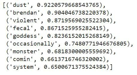
model.wv.most_similar(‘disaster’)
Output —
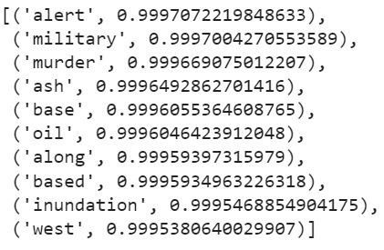
List of tuples of words and their predicted probability
The embedding vector of ‘disaster’ —
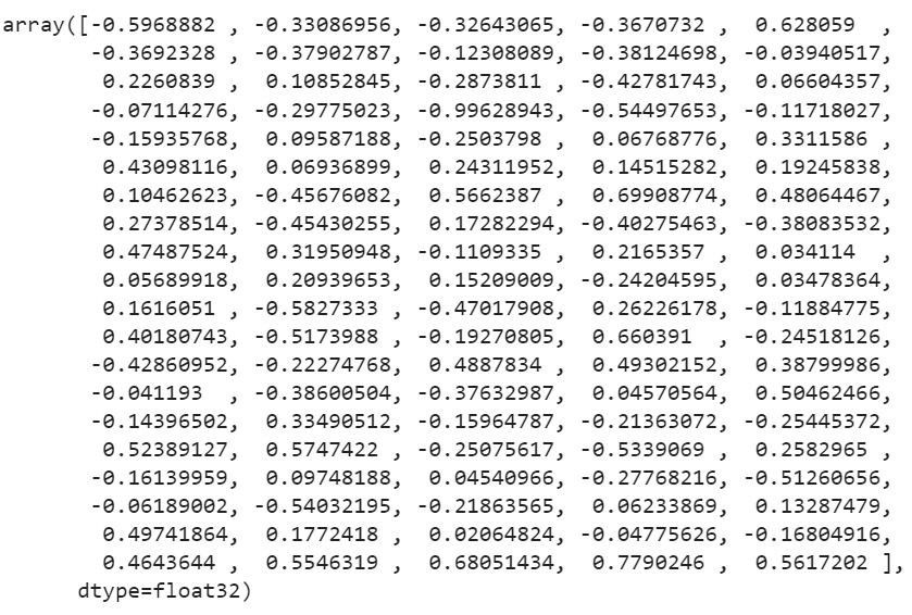
dimensionality = 100
Challenges with the bag of words and TF-IDF
Now let’s discuss the challenges with the two text vectorization techniques we have discussed till now.
In BOW, the size of the vector is equal to the number of elements in the vocabulary. If most of the values in the vector are zero then the bag of words will be a sparse matrix. Sparse representations are harder to model both for computational reasons and also for informational reasons.
Also, in BOW there is a lack of meaningful relations and no consideration for the order of words. Here’s more that adds to the challenge with this word embedding technique.
-
Massive amount of weights: Large amounts of input vectors invite massive amounts of weight for a neural network.
-
No meaningful relations or consideration for word order: The bag of words does not consider the order in which the words appear in the sentences or a text.
-
Computationally intensive: With more weight comes the need for more computation to train and predict.
While the TF-IDF model contains the information on the more important words and the less important ones, it does not solve the challenge of high dimensionality and sparsity, and unlike BOW it also makes no use of semantic similarities between words.
GloVe: Global Vector for word representation
GloVe method of word embedding in NLP was developed at Stanford by Pennington, et al. It is referred to as global vectors because the global corpus statistics were captured directly by the model. It finds great performance in world analogy and named entity recognition problems.
This technique reduces the computational cost of training the model because of a simpler least square cost or error function that further results in different and improved word embeddings. It leverages local context window methods like the skip-gram model of Mikolov and Global Matrix factorization methods for generating low dimensional word representations.
Latent semantic analysis (LSA) is a Global Matrix factorization method that does not do well on world analogy but leverages statistical information indicating a sub-optimal vector space structure.
On the contrary, the skip-gram method performs better on the analogy task. However, it does not utilize the statistics of the corpus properly because of no training on global co-occurrence counts.
So, unlike Word2Vec, which creates word embeddings using local context, GloVe focuses on global context to create word embeddings which gives it an edge over Word2Vec. In GloVe, the semantic relationship between the words is obtained using a co-occurrence matrix.
Consider two sentences —
I am a data science enthusiast
I am looking for a data science job
The co-occurrence matrix involved in GloVe would look like this for the above sentences —
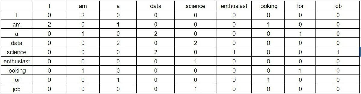
Window Size = 1
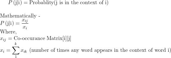
Each value in this matrix represents the count of co-occurrence with the corresponding word in row/column. Observe here — this co-occurrence matrix is created using global word co-occurrence count (no. of times the words appeared consecutively; for window size=1). If a text corpus has 1m unique words, the co-occurrence matrix would be 1m x 1m in shape. The core idea behind GloVe is that the word co-occurrence is the most important statistical information available for the model to ‘learn’ the word representation.
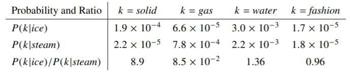
Let’s now see an example from Stanford’s GloVe paper of how the co-occurrence probability rations work in GloVe. “For example, consider the co-occurrence probabilities for target words ice and steam with various probe words from the vocabulary. Here are some actual probabilities from a corpus of 6 billion words:”
Here,
Let’s take k = solid i.e, words related to ice but unrelated to steam. The expected Pik /Pjk ratio will be large. Similarly, for words k which are related to steam but not to ice, say k = gas, the ratio will be small. For words like water or fashion, which are either related to both ice and steam or neither to both respectively, the ratio should be approximately one.
The probability ratio is able to better distinguish relevant words (solid and gas) from irrelevant words (fashion and water) than the raw probability. It is also able to better discriminate between two relevant words. Hence in GloVe, the starting point for word vector learning is ratios of co-occurrence probabilities rather than the probabilities themselves.
Enough of the theory. Time for the code!
Import Libraries
import nltk
import re
from nltk.corpus import stopwords
from glove import Corpus, Glove
Text Preprocessing
#GloVe inputs a corpus of documents splitted into constituent words
corpus = []
for i in range(0,len(X)):
 tweet = re.sub(“[^a-zA-Z]”,” “,X[i])
 tweet = tweet.lower()
 tweet = tweet.split()
 corpus.append(tweet)
Train the word Embeddings
corpus = Corpus()
corpus.fit(text_corpus,window = 5)
glove = Glove(no_components=100, learning_rate=0.05)
#no_components = dimensionality of word embeddings = 100
glove.fit(corpus.matrix, epochs=100, no_threads=4, verbose=True)
glove.add_dictionary(corpus.dictionary)
Find most similar -
glove.most_similar(“storm”,number=10)
Output —
List of tuples of words and their predicted probability
BERT (Bidirectional encoder representations from transformers)
This natural language processing (NLP) based language algorithm belongs to a class known as transformers. It comes in two variants namely BERT-Base, which includes 110 million parameters, and BERT-Large, which has 340 million parameters.
It relies on an attention mechanism for generating high-quality world embeddings that are contextualized. So when the embedding goes through the training process, they are passed through each BERT layer so that its attention mechanism can capture the word associations based on the words on the left and those on the right.
It is an advanced technique in comparison to the discussed above as it creates better word embedding. The credit goes to the pre-trend model on Wikipedia data sets and massive word corpus. This technique can be further improved for task-specific data sets by fine-tuning the embeddings.
It finds great application in language translation tasks.
Conclusion
Word embeddings can train deep learning models like GRU, LSTM, and Transformers, which have been successful in NLP tasks such as sentiment classification, name entity recognition, speech recognition, etc.
Here’s a final checklist for a recap.
- Bag of words: Extracts features from the text
- TF-IDF: Information retrieval, keyword extraction
- Word2Vec: Semantic analysis task
- GloVe: Word analogy, named entity recognition tasks
- BERT: language translation, question answering system
In this blog, we discussed the two techniques for vectorizations in NLP: the Bag of Words and TF-IDF, their drawbacks, and how word-embedding techniques like GloVe and Word2Vec overcome their drawbacks by dimensionality reduction and context similarity. With all said above, you would have a better understanding of how word embeddings benefits your day-to-day life as well.
Word embeddings is one of the most used techniques in natural language processing (NLP). It’s often said that the performance and ability of SOTA models wouldn’t have been possible without word embeddings. It’s precisely because of word embeddings that language models like RNNs, LSTMs, ELMo, BERT, AlBERT, GPT-2 to the most recent GPT-3 have evolved at a staggering pace.
These algorithms are fast and can generate language sequences and other downstream tasks with high accuracy, including contextual understanding, semantic and syntactic properties, as well as the linear relationship between words.
At the core, these models use embedding as a method to extract patterns from text or voice sequences. But how do they do that? What is the exact mechanism and the math behind word embeddings?
In this article, we’ll explore some of the early neural network techniques that let us build complex algorithms for natural language processing. For certain topics, there will be a link to the paper and a colab notebook attached to it, so that you can understand the concepts through trying them out. Doing so will help you learn quicker.
Topics we’ll be covering:
- What are word embeddings?
- Neural Language Model
- Word2Vec
- Skipgrams
- Continuous bag of words
- On softmax function
- Improving approximation
- Softmax-based approaches
- Hierarchical Softmax
- Sampling-based approaches
- Noise contrastive estimation
- Negative sampling
- Softmax-based approaches
What are word embeddings?
Word embeddings are a way to represent words and whole sentences in a numerical manner. We know that computers understand the language of numbers, so we try to encode words in a sentence to numbers such that the computer can read it and process it.
But reading and processing are not the only things that we want computers to do. We also want computers to build a relationship between each word in a sentence, or document with the other words in the same.
We want word embeddings to capture the context of the paragraph or previous sentences along with capturing the semantic and syntactic properties and similarities of the same.
For instance, if we take a sentence:
“The cat is lying on the floor and the dog was eating”,
…then we can take the two subjects (cat and dog) and switch them in the sentence making it:
“The dog is lying on the floor and the cat was eating”.
In both sentences, the semantic or meaning-related relationship is preserved, i.e. cat and dog are animals. And the sentence makes sense.
Similarly, the sentence also preserved syntactic relationship, i.e. rule-based relationship or grammar.
In order to achieve that kind of semantic and syntactic relationship we need to demand more than just mapping a word in a sentence or document to mere numbers. We need a larger representation of those numbers that can represent both semantic and syntactic properties.
We need vectors. Not only that, but learnable vectors.
In a mathematical sense, a word embedding is a parameterized function of the word:
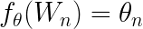
where is the parameter and W is the word in a sentence.
A lot of people also define word embedding as a dense representation of words in the form of vectors.
For instance, the word cat and dog can be represented as:
W(cat) = (0.9, 0.1, 0.3, -0.23 … )
W(dog) = (0.76, 0.1, -0.38, 0.3 … )
Now, hypothetically speaking, if the model is able to preserve the contextual similarity, then both words will be close in a vector space.

So far we’ve dealt with two words (cat and dog), but what if there are more words? The job of a work embedding model is to cluster similar information and establish a relationship between them.
As you can see, word embeddings clusters similar words together.
There are a lot of shallow algorithms present that work well for clustering. Why do we need neural networks?
One of the biggest misconceptions is that word embeddings require deep neural networks. As we build different word embedding models, you will see that for all the embeddings, the model is a shallow neural network, and some are linear models as well.
The reasons we use neural networks to create word embeddings are:
- It’s useful in finding nearest neighbors in the embedding space.
- It can be used as an input to supervised learning tasks.
- It creates a mapping of discrete variables, such as words to a vector, of continuous variables.
- It also tackles the curse of dimensionality.
Training, Visualizing, and Understanding Word Embeddings: Deep Dive Into Custom Datasets
Neural Language Model
Word embeddings were proposed by Bengio et. al. (2001, 2003) to tackle what’s known as the curse of dimensionality, a common problem in statistical language modelling.
It turns out that Bengio’s method could train a neural network such that each training sentence could inform the model about a number of semantically available neighboring words, which was known as distributed representation of words. The neural network not established relationships between different words, but it also preserved relationships in terms of both semantic and syntactic properties.

This introduced a neural network architecture approach that laid the foundation for many current approaches.
This neural network has three components:
- An embedding layer that generates word embedding, and the parameters are shared across words.
- A hidden layer of one or more layers, which introduces non-linearity to the embeddings.
- A softmax function that produces probability distribution over all the words in the vocabulary.
Let’s understand how a neural network language model works with the help of code.
(here are links to the Notebook and original Paper)
Step 1: Indexing the words. We start by indexing the words. For each word in the sentence, we’ll assign a number to it.
word_list = " ".join(raw_sentence).split()
word_list = list(set(word_list))
word2id = {w: i for i, w in enumerate(word_list)}
id2word = {i: w for i, w in enumerate(word_list)}
n_class = len(word2id)
Step 2: Building the model.
We will build the model exactly as described in the paper.
class NNLM(nn.Module):
   def __init__(self):
       super(NNLM, self).__init__()
       self.embeddings = nn.Embedding(n_class, m)

       self.hidden1 = nn.Linear(n_step * m, n_hidden, bias=False)
       self.ones = nn.Parameter(torch.ones(n_hidden))

       self.hidden2 = nn.Linear(n_hidden, n_class, bias=False)
       self.hidden3 = nn.Linear(n_step * m, n_class, bias=False)

       self.bias = nn.Parameter(torch.ones(n_class))

   def forward(self, X):
       X = self.embeddings(X)
       X = X.view(-1, n_step * m)
       tanh = torch.tanh(self.d + self.hidden1(X))
       output = self.b + self.hidden3(X) + self.hidden2(tanh)
       return output
We’ll start by initializing an embedding layer. An embedding layer is a lookup table.
Once the input index of the word is embedded through an embedding layer, it’s then passed through the first hidden layer with bias added to it. The output of these two is then passed through a tanh function.
If you remember from the diagram in the original paper, the output from the embedded layer is also passed into the final hidden layer, where the output of the tanh is summed together.
output = self.b + self.hidden3(X) + self.hidden2(tanh)
Now, in the last step we will calculate the probability distribution over the entire vocabulary.
Step 3: Loss and optimization function.
Now that we have the output from the model, we need to make sure that we pass it through the softmax function to get the probability distribution.
We’re using cross entropy loss.
criterion = nn.CrossEntropyLoss()
The cross entropy loss is made up of two equations: log softmax function, and negative log likelihood loss or NLLLoss. The former calculates the softmax normalization, while the latter calculates the negative log likelihood loss.
For optimization, we use Adam optimizer.
Cross-Entropy Loss and Its Applications in Deep Learning
Step 4: Training.
Finally, we train the model.
In a nutshell, word embeddings can be defined as a dense representation of words in the form of vectors in low-dimensional space. These embeddings are accompanied by learnable vectors, or parameterized functions. They update themselves during backpropagation using a loss function, and try to find a good relationship between words, preserving both semantic and synaptic properties.

“As it turned out that neural network based models significantly outperformed statistical based models” Mikolov et. al. (2013).
Word2Vec
The approach introduced by Bengio opened new opportunities for NLP researchers to modify the technique and the architecture itself, to create a method that’s computationally less expensive. Why?
The method that Bengio et al proposed takes words for the vocabulary, and feeds them into a feed forward neural network with an embedding layer, hidden layer(s) and a softmax function.
These embeddings have associated learnable vectors, which optimize themselves through back propagation. Essentially, the first layer of the architecture yields word embeddings, since it’s a shallow network.
The problem with this architecture is that it’s computationally expensive between the hidden layer and the projection layer. The reason for it is complex:
- The values produced in the projection are dense.
- The hidden layer computes probability distribution for all the words in the vocabulary.
To address this issue, researchers (Mikolov et al. in 2013) came along with a model called ‘Word2Vec’.
A Word2Vec model essentially addresses the issues of Bengio’s NLM.
It removes the hidden layer altogether, but the projection layer is shared for all words, just like Bengio’s model. The downside is that this simple model without a neural network won’t be able to represent data as precisely as the neural network can, if there’s less data.
On the other hand, with a larger dataset, it can represent the data precisely in the embedding space. Along with it, it also reduces complexity, and the model can be trained in larger datasets.
Mikolov et al. in 2013 proposed two models:
- Continuous Bag-of-Words Model
- Continuous Skip-gram Model
Continuous bag-of-words model
A Continuous Bag-of-Words or CBOW model basically takes ‘n’ words before and after the target word (wt), and predicts the latter. n can be any number.
For instance, if n=2 and the sentence is ‘the dog is playing in the park”, then the words fed into the model will be ([the, dog, is, in, the, park] ), followed by the target word ‘playing’.
This model takes out the complexity of calculating probability distribution over all the words in the vocabulary by just calculating the log2(V), where V is the vocabulary size. Hence this model is faster and efficient.
Let’s understand how a CBOW model works with the help of code.
(here are links to the Notebook and original paper)
To begin with, we won’t change the word encoding method to numbers. That will stay the same.
Step 1: Define a function to create a context window with n words from the right and left of the target word.
def CBOW(raw_text, window_size=2):
   data = []
   for i in range(window_size, len(raw_text) - window_size):
       context = [raw_text[i - window_size], raw_text[i - (window_size - 1)], raw_text[i + (window_size - 1)], raw_text[i + window_size]]
       target = raw_text[i]
       data.append((context, target))

   return data
The function should take two arguments: data and window size. The window size will define how many words we are supposed to take from the right and from the left.
The for loop: for i in range(window_size, len(raw_text) – window_size): iterates through a range starting from the window size, i.e. 2 means it will ignore words in index 0 and 1 from the sentence, and end 2 words before the sentence ends.
Inside the for loop, we try separate context and target words and store them in a list.
For example, if the sentence is “The dog is eating and the cat is lying on the floor”, CBOW with window 2 will consider words ‘The’, ‘dog’, ‘eating’ and ‘and’. Essentially making the target word ‘is’.
Let i = window size = 2, then:
context = [raw_text[2 - 2], raw_text[2 - (2 - 1)], raw_text[i + (2 - 1)], raw_text[i + 2]]

target = raw_text[2]
Let’s call the function and see the output.
data = CBOW(raw_text)
print(data[0])
Output:
(['The', 'dog', 'eating', 'and'], 'is')
Step 2: Build the model.
Building a CBOW is similar to building the NNLM we did earlier, but actually much simpler.
In the CBOW model, we reduce the hidden layer to only one. So all together we have: an embedding layer, a hidden layer which passes through the ReLU layer, and an output layer.
class CBOW_Model(torch.nn.Module):
   def __init__(self, vocab_size, embedding_dim):
       super(CBOW_Model, self).__init__()

       self.embeddings = nn.Embedding(vocab_size, embedding_dim)
       self.linear1 = nn.Linear(embedding_dim, 128)
       self.activation_function1 = nn.ReLU()

       self.linear2 = nn.Linear(128, vocab_size)


   def forward(self, inputs):
       embeds = sum(self.embeddings(inputs)).view(1,-1)
       out = self.linear1(embeds)
       out = self.activation_function1(out)
       out = self.linear2(out)
       return out
This model is pretty straightforward. The context words index is fed into the embedding layers, which is then passed through the hidden layer followed by the nonlinear activation layer, i.e. ReLU, and finally we get the output.
Step 3: Loss and optimization function.
Similar to NNLM, we use the same technique for calculating probability distribution over all the words in the vocabulary, ie. nn.CrossEntropyLoss().
For optimization, we use Stochastic Gradient Descent. You can use Adam optimizer as well. In NLP, Adam is the go-to optimizer because it converges faster than SGD.
optimizer = torch.optim.SGD(model.parameters(), lr=0.01)
Step 4: Training
Training is the same as the NNLM model.
for epoch in range(50):
   total_loss = 0

   for context, target in data:

       context_vector = make_context_vector(context, word_to_ix)

       output = model(context_vector)

       target = torch.tensor([word_to_ix[target]])
       total_loss += loss_function(output, target)


   optimizer.zero_grad()
   total_loss.backward()
   optimizer.step()
make_context_vector turns words into numbers.
It’s worth noting that authors of this paper found that NNLM preserves linear relationships between words with similarity. For example, ‘king’ and ‘queen’ are the same as ‘men’ and ‘women’, i.e. NNLM preserves gender linearity.
Similarly, models such as CBOW and any neural network model that we’ll be discussing next will preserve linear relationships, even though we specifically define nonlinearity in the neural network.
Continuous skip-gram model
Continuous skip-gram, or skip-gram, is similar to CBOW. Instead of predicting the target word (wt), it predicts the word surrounding it with context. The training objective is to learn representations, or embeddings, that are good at predicting nearby words.
It also takes an “n” number of words. For instance, if n=2 and the sentence is ‘the dog is playing in the park”, then the word fed into the model will be playing, and the target words will be (the, dog, is, in, the, park).
Let’s understand how a skip-gram model works with the help of code.
(here are links to the Notebook and original paper)
A skipgram model is the same as the CBOW model with one difference. The difference lies in creating the context and the target word.
Step 1: Setting target and context variable.
Since skipgram takes a single context word and n number of target variables, we just need to flip the CBOW from the previous model.
def skipgram(sentences, window_size=1):
   skip_grams = []
   for i in range(window_size, len(word_sequence) - window_size):
       target = word_sequence[i]
       context = [word_sequence[i - window_size], word_sequence[i + window_size]]
       for w in context:
           skip_grams.append([target, w])

   return skip_grams
As you can see, the function is almost the same.
Here, you need to understand that when the window size is 1, we take one word before and after the target word.
When we call the function, the output looks something like this:
print(skipgram(word_sequence)[0:2])
Output:
[['my', 'During'], ['my', 'second']]
As you can see, the target word is ‘my’ and the two words are ‘During’ and ‘second’.
Essentially, we’re trying to create a pair of words such that each pair will contain a target word. Depending on the context window, it will contain the neighboring words.
Step 2: Building the model.
The model is pretty straightforward.
class skipgramModel(nn.Module):
   def __init__(self):
       super(skipgramModel, self).__init__()
       self.embedding = nn.Embedding(voc_size, embedding_size)
       self.W = nn.Linear(embedding_size, embedding_size, bias=False)
       self.WT = nn.Linear(embedding_size, voc_size, bias=False)

   def forward(self, X):
       embeddings = self.embedding(X)
       hidden_layer = nn.functional.relu(self.W(embeddings))
       output_layer = self.WT(hidden_layer)
       return output_layer
The loss function and optimisation remains the same.
criterion = nn.CrossEntropyLoss()
optimizer = optim.Adam(model.parameters(), lr=0.001)
Once we’ve defined everything, we can train the model.
for epoch in range(5000):
        input_batch, target_batch = random_batch()
        input_batch = torch.Tensor(input_batch)
        target_batch = torch.LongTensor(target_batch)

        optimizer.zero_grad()
        output = model(input_batch)


        loss = criterion(output, target_batch)
        if (epoch + 1) % 1000 == 0:
            print('Epoch:', '%04d' % (epoch + 1), 'cost =', '{:.6f}'.format(loss))

        loss.backward()
        optimizer.step()
The skip-gram model increases computational complexity because it has to predict nearby words based on the number of neighboring words. The more distant words tend to be slightly less related to the current word.
Summary so far:
- Neural Network Language Model (NNLM) or Bengio’s model outperforms the earlier statistical model like the n-gram model.
- NNLM also tackles the curse of dimensionality and preserves contextual, linguistic regularities and patterns through its distributed representation.
- NNLM is computationally expensive.
- Word2Vec models tackles computational complexity by removing the hidden layer and sharing the weights
- The downside of Word2Vec is it does not have a neural network which makes it hard to represent the data but the upside is that if it can be trained on a large number of data then because it is much more efficient than neural networks it is possible to compute very accurate high dimensional word vectors.
- Word2Vec has two models: CBOW and Skipgram. The former is faster than the latter.
On softmax function
So far, you’ve seen how the softmax function plays a vital role in predicting the words around a given context. But it suffers from a complexity issue.
Recall the equation of softmax function:

Where wt is the target word, c is the context words, and y is the output for each target word.
If you look at the equation above, the complexity of the softmax function arises when the number of predictors is high. If i=3, then the softmax function will return a probability distribution over three categories.
But, in NLP we usually deal with thousands, sometimes millions of words. Getting a probability distribution over that many words will make the computation really expensive and slow.
Keep in mind that softmax functions return the exact probability distribution, so they tend to get slower with increasing parameters. For each word (wt), it sums over the entire vocabulary in the denominator.
So what are the different approaches that will make computation inexpensive and fast, while making sure that the approximation is not compromised?
In the next section, we’ll cover different approaches that can reduce the computational time. Instead of getting exact probabilities over the full vocabulary, we’ll try to approximate over the full vocabulary, or even a sample vocabulary. This reduces complexity and increases processing speed.
We will discuss two approaches: softmax-based approaches and sampling-based approaches.
Gumbel Softmax Loss Function Guide + How to Implement it in PyTorch
Improving predictive functions
In this section, we explore three possible methods for improving prediction, by modifying the softmax function for approximating better results, and replacing the softmax with new methods.
Softmax-based approaches
Softmax-based approaches are more inclined towards modifying the softmax to get a better approximation of the predicted word, rather than eliminating it altogether. We will discuss two methods: hierarchical softmax approach and CNN approach.
Hierarchical softmax
Hierarchical softmax was introduced by Morin and Bengio in 2005, as an alternative to the full softmax function, where it replaces it with a hierarchical layer. It borrows the technique from the binary huffman tree, which reduces the complexity of calculating the probability from the whole vocabulary V to log2(V), i.e. binary.
Coding a huffman tree is very complicated. I’ll try to explain it without using code, but you can find the notebook here and try it out.
To understand the H-softmax, we need to understand the workings of the huffman tree.
The huffman tree is a binary tree that takes the words from the vocabulary; based on their frequency in the document, it creates a tree.
Take for example this text: “the cat is eating and the dog is barking”. In order to create a huffman tree, we need to calculate the frequency of words from the whole vocabulary.
word_to_id = {w:i for i, w in enumerate(set(raw_text))}
id_to_word = {i:w for w, i in word_to_id.items()}
word_frequency = {w:raw_text.count(w) for w,i in word_to_id.items()}
print(word_frequency)
Output:

{'and': 1, 'barking': 1, 'cat': 1, 'dog': 1, 'eating': 1, 'is': 2, 'the': 2}
The next step is to create a huffman tree. The way we do it is by taking the least frequent word. In our example, we have a lot of words that are occurring only once, so we’re free to take any two. Let’s take ‘dog’ and ‘and’. We will then join the two leaf nodes by a parent node, and add the frequency.

In the next step, we’ll take another word that is least frequent (again, the word that occurs only once) and we’ll put it beside the node that has the sum of two. Remember that less frequent words go to the left side, and more frequent words go to the right side.

Similarly, we’ll keep on building the words until we’ve used all the words from the vocabulary.

Remember, all the words with the least frequency are at the bottom.
print(Tree.wordid_code)
Output:
{0: [0, 1, 1],
 1: [0, 1, 0],
 2: [1, 1, 1, 1],
 3: [1, 1, 1, 0],
 4: [0, 0],
 5: [1, 1, 0],
 6: [1, 0]}
Once the tree is created, we can then start the training.
In the huffman tree, we no longer calculate the output embeddings w`. Instead, we try to calculate the probability of turning right or left at each leaf node, using a sigmoid function.
p(right | n,c)=σ(h⊤w′n), where n is the node and c is the context.
As you will find in the code below, a sigmoid function is used to decide whether to go right or to left. It’s also important to know that the probabilities of all the words should sum up to 1. This ensures that the H-softmax has a normalized probability distribution over all the words in the vocabulary.
class SkipGramModel(nn.Module):
   def __init__(self, emb_size, emb_dimension):
       super(SkipGramModel, self).__init__()
       self.emb_size = emb_size
       self.emb_dimension = emb_dimension
       self.w_embeddings = nn.Embedding(2*emb_size-1, emb_dimension, sparse=True)
       self.v_embeddings = nn.Embedding(2*emb_size-1, emb_dimension, sparse=True)
       self._init_emb()

   def _init_emb(self):
       initrange = 0.5 / self.emb_dimension
       self.w_embeddings.weight.data.uniform_(-initrange, initrange)
       self.v_embeddings.weight.data.uniform_(-0, 0)

   def forward(self, pos_w, pos_v,neg_w, neg_v):

       emb_w = self.w_embeddings(torch.LongTensor(pos_w))
       neg_emb_w = self.w_embeddings(torch.LongTensor(neg_w))
       emb_v = self.v_embeddings(torch.LongTensor(pos_v))
       neg_emb_v = self.v_embeddings(torch.LongTensor(neg_v))

       score = torch.mul(emb_w, emb_v).squeeze()
       score = torch.sum(score, dim=1)
       score = F.logsigmoid(-1 * score)
       neg_score = torch.mul(neg_emb_w, neg_emb_v).squeeze()
       neg_score = torch.sum(neg_score, dim=1)
       neg_score = F.logsigmoid(neg_score)

       loss = -1 * (torch.sum(score) + torch.sum(neg_score))
       return loss
Sampling-based approaches
Sampling-based approaches completely eliminate the softmax layer.
We’ll discuss two approaches: noise contrastive estimation, and negative sampling.
Noise contrastive estimation
Noise contrastive estimation (NCE) is an approximation method that replaces the softmax layer and reduces the computational cost. It does so by converting the prediction problem into a classification problem.
This section will contain a lot of mathematical explanations.
NCE takes an unnormalised multinomial function (i.e. the function that has multiple labels and its output has not been passed through a softmax layer), and converts it to a binary logistic regression.
In order to learn the distribution to predict the target word (wt) from some specific context (c), we need to create two classes: positive and negative. The positive class contains samples from training data distribution, while the negative class contains samples from a noise distribution Q, and we label them 1 and 0 respectively. Noise distribution is a unigram distribution of the training set.
For every target word given context, we generate sample noise from the distribution Q as Q(w), such that it’s k times more frequent than the samples from the data distribution P(w | c).
These two probability distributions can be represented as the sum of each other because we are effectively sampling words from the two distributions. Hence,

As mentioned earlier, NCE is a binary classifier which consists of a true label as ‘1’ and false label as ‘0’. Intuitively,
When y=1,

When y=0,

Our aim is to develop a model with parameters θ, such that given a context c, its predicted probability P(w,c) approximates the original data distribution Pd(w,c).

Generally, the noise distribution is approximated by sampling. We do that by generating k noise samples {wij}:

Where Zθ(c) is a normalizing term from the softmax, and you recall this is what we are trying to eliminate. The way we can eliminate Zθ(c) is by making it a learnable parameter. Essentially, we transform the softmax function from absolute value, i.e. the value which sums over all the words in vocabulary again and again, to a dynamic value which changes to find a better for itself – it’s learnable.
But, as it turns out, Mnih et al. (2013) stated that Zθ(c) can be fixed at 1. Even though it’s static again but it normalizes quite well, Zoph et al. (2016) found that Zθ(c)=1 produces a model with low variance.
We can replace Pθ(w | c) with exp(sθ(w | c)) such that the loss function can be written as:
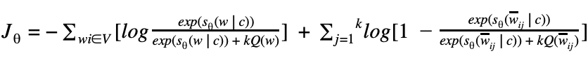
One thing to keep in mind is that as we increase the number of noise samples k, the NCE derivative approaches the likelihood gradient, or the softmax function of the normalised model.
In conclusion, NCE is a way of learning a data distribution by comparing it against a noise distribution, and modifying the learning parameters such that the model Pθ is almost equal to Pd.
Negative sampling
It’s important to understand NCE, because negative sampling is the modified version of the same. It’s a more simplified version as well.
To begin with, we learned that as we increase the number of noise samples k, the NCE derivative approaches the likelihood gradient, or the softmax function of the normalised model.
The way negative sampling works is, it gets rid of the noise by replacing it with 1. Intuitively,
When y=1,

In negative sampling we use a sigmoid function, so we’ll transform the above equation to:

We know that Pθ(w | c) is replaced with exp(sθ(w | c)).
Therefore,

This makes the equation shorter. It has to compute 1 instead of noise, so the equation becomes computationally efficient. But why do we care to simplify NCE?
One reason is that we’re concerned with the high representation of the word vector, so it can simplify the model as long as the word embeddings produced by the model retain their quality.
If we replace the final NCE equation with the equation above, we get:

Since log(1)=0,
therefore,

Since we’re dealing with sigmoid function i.e.

we can modify the equation above to:

(Here are the links to the Notebook and original paper)
Final thoughts and conclusion
We explored the evolution of neural-based modelling for NLP or machine translation. We covered word embedding, a method to find semantic, syntactic and linear relationship in the vocabulary. Although some of the methods mentioned earlier are no longer used, they lay the basic foundation of the subject, and make further learning easier.
We saw how Begio and his team introduced neural language models to find better representation through their word embedding method, followed by how Mikolov and his team modified Begio’s method and introduced a computationally less expensive method by removing the hidden layer. Although the word2vec model is a simple model, it became computationally expensive once the vocabulary size increased.
Different methods were introduced to rectify the issue of complexities, and the three models that we saw later in the post addressed the issue with the softmax function.
In the end, we saw how negative sampling outranks all the two methods (hierarchical softmax and NCE), and modifies word2vec model with a much more efficient approximation technique that captures better representation like semantic, syntactic, and preserves linear representation as well reduces the computational cost.
Word embedding opened new doors for NLP research and development. These models work well, but they still lack conceptual understanding. It was only in 2018 that Peters et. al. introduced ELMo: Embeddings from Language Model, which linked the missing piece of finding contextual representation through word embeddings.
For better understanding and clarity, check out the notebooks for each topic.
Resources
- On word embeddings – Part 1
- On word embeddings – Part 2: Approximating the Softmax
- Noise Contrastive Estimation
- The Illustrated Word2vec
- Distributed Representations of Words and Phrases and their Compositionality
- Efficient Estimation of Word Representations in Vector Space
- A Neural Probabilistic Language Model
- Notes on Noise Contrastive Estimation and Negative Sampling
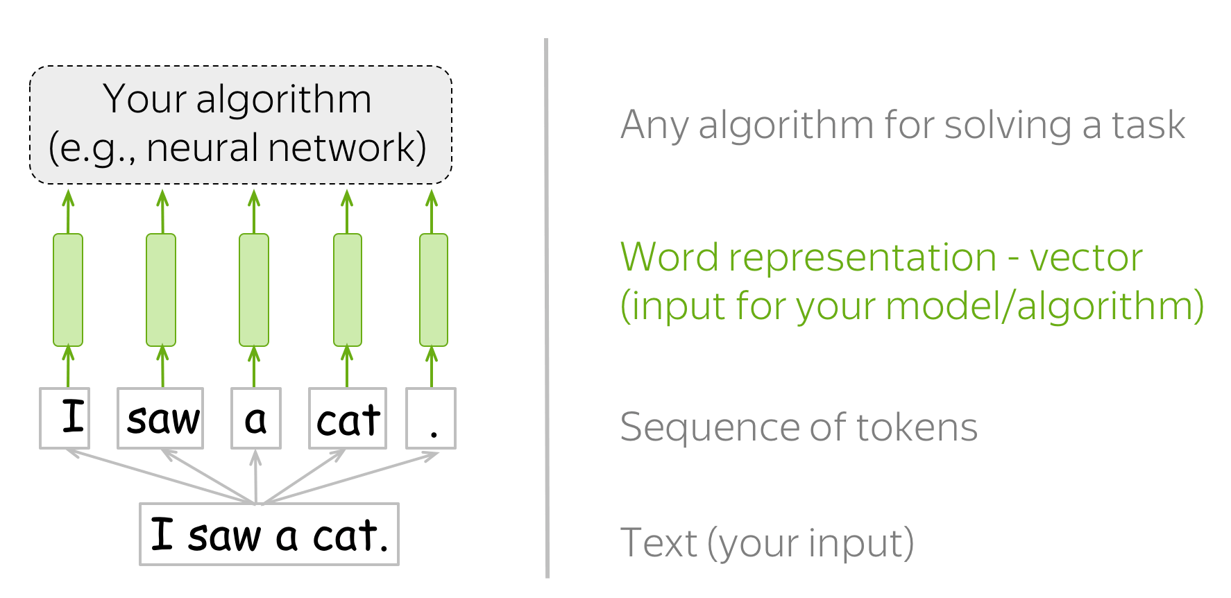
The way machine learning models «see» data is different from how we (humans) do. For example, we can easily
understand the text «I saw a cat»,
but our models can not — they need vectors of features.
Such vectors, or word embeddings, are representations of words which can be fed into your model.
How it works: Look-up Table (Vocabulary)
In practice, you have a vocabulary of allowed words; you choose this vocabulary in advance.
For each vocabulary word, a look-up table contains its embedding. This embedding can be found
using the word index in the vocabulary (i.e., you
to look up the embedding in the table using word index).
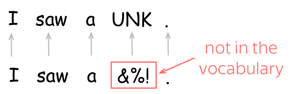
To account for unknown words (the ones which are not in the vocabulary), usually a vocabulary
contains a special token
UNK. Alternatively, unknown tokens
can be ignored
or assigned a zero vector.
The main question of this lecture is: how do we get these word vectors?
Represent as Discrete Symbols: One-hot Vectors
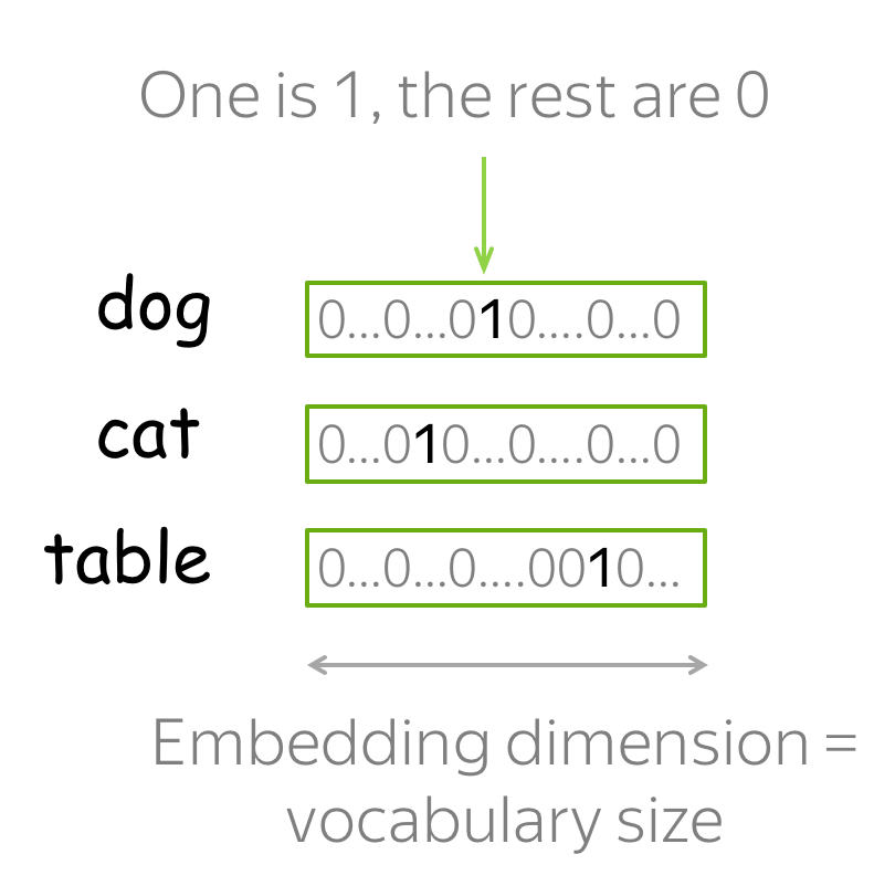
The easiest you can do is to represent words as one-hot vectors: for the i-th word in the vocabulary,
the vector has 1 on the i-th dimension and 0 on the rest. In Machine Learning, this is the most simple way to represent
categorical features.
You probably can guess why one-hot vectors are not the best way to represent words. One of the problems is that
for large vocabularies, these vectors will be very long: vector dimensionality is equal to the vocabulary size.
This is undesirable in practice, but this problem is not the most crucial one.
What is really important, is that these vectors know nothing
about the words they represent. For example, one-hot vectors «think» that
cat is as close to
dog as it is to
table!
We can say that one-hot vectors do not capture meaning.
But how do we know what is meaning?
Distributional Semantics
To capture meaning of words in their vectors, we first need to define
the notion of meaning that can be used in practice.
For this, let us try to understand how we, humans, get to know which words have similar meaning.
![]()
![]()
Once you saw how the unknown word used in different contexts,
you were able to understand it’s meaning.
How did you do this?
The hypothesis is that your brain searched for other words
that can be used in the same contexts, found some (e.g., wine), and
made a conclusion that tezgüino has meaning
similar to those other words.
This is the distributional hypothesis:
Words which frequently appear in similar contexts have
similar meaning.
Lena:
Often you can find it formulated as «You shall know a word by the company it keeps» with the reference
to J. R. Firth in 1957, but
actually there
were a lot more people
responsible, and much earlier. For example,
Harris, 1954.
This is an extremely valuable idea: it can be used in practice to make word vectors capture
their meaning. According to the distributional hypothesis, «to capture meaning» and
«to capture contexts» are inherently the same.
Therefore,
all we need to do is to put information about word
contexts into word representation.
Main idea: We need to put information about word
contexts into word representation.
All we’ll be doing at this lecture is looking at different ways to do this.
Count-Based Methods
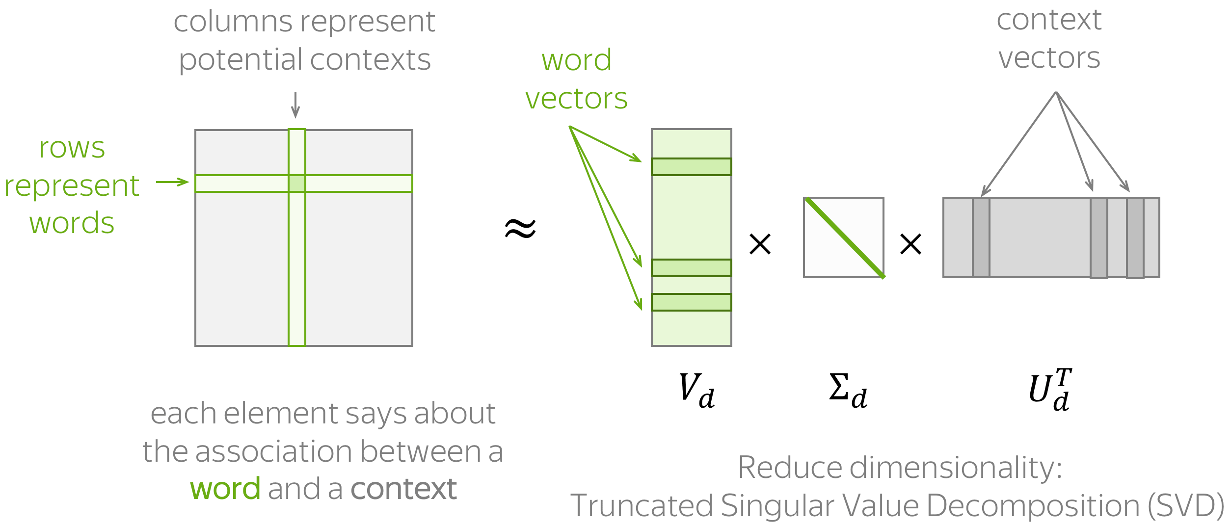
Let’s remember our main idea:
Main idea:
We have to put information about contexts into word vectors.
Count-based methods take this idea quite literally:
How:
Put this information manually based on global corpus statistics.
The general procedure is illustrated above and consists of the two steps: (1)
construct a word-context matrix, (2) reduce its dimensionality. There are two reasons to reduce dimensionality.
First, a raw matrix is very large. Second, since a lot of words appear in only a few of possible contexts,
this matrix potentially has a lot of uninformative elements (e.g., zeros).
To estimate
similarity between words/contexts, usually you need to evaluate
the dot-product of normalized word/context vectors (i.e., cosine similarity).
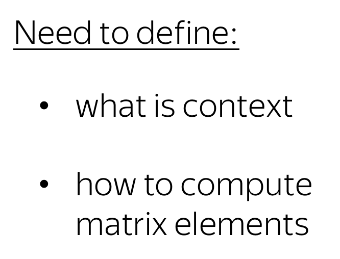
To define a count-based method, we need to define two things:
- possible contexts (including what does it mean that a word appears in a context),
- the notion of association, i.e., formulas for computing matrix elements.
Below we provide a couple of popular ways of doing this.
Simple: Co-Occurence Counts
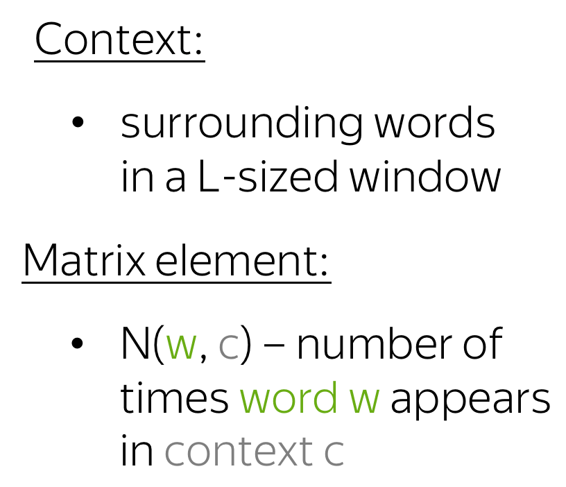
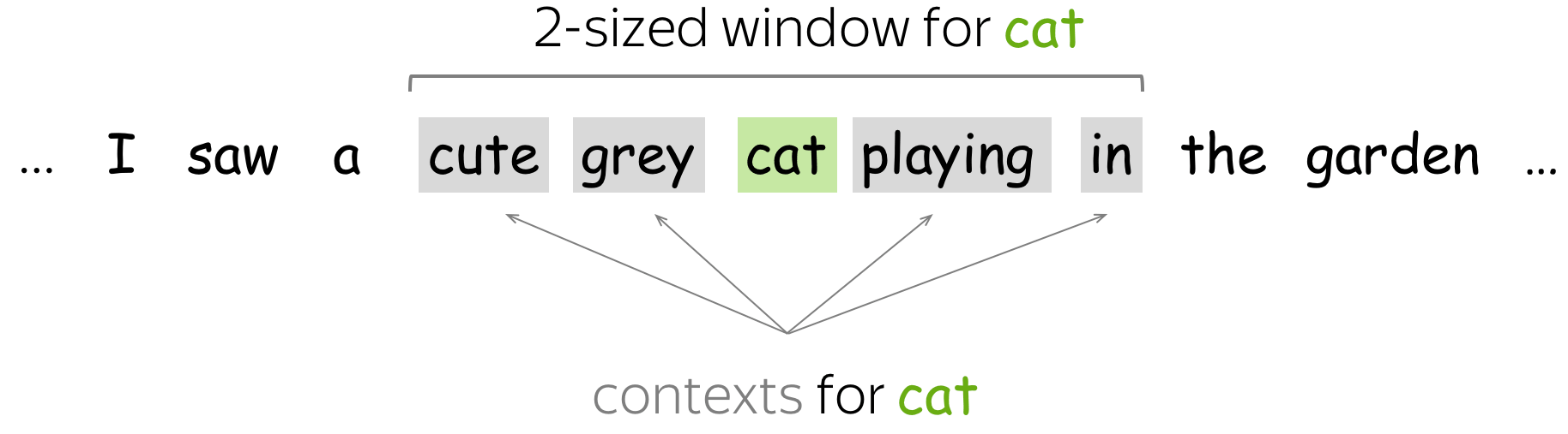
The simplest approach is to define contexts as each word in an L-sized window.
Matrix element for a word-context pair (w, c) is the number of times w appears in context c.
This is the very basic (and very, very old) method for obtaining embeddings.
![]()
The (once) famous HAL model (1996)
is also a modification of this approach.
Learn more from this exercise
in the Research Thinking section.
Positive Pointwise Mutual Information (PPMI)
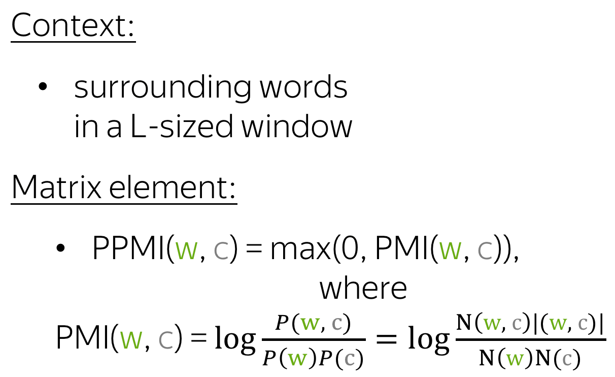
Here contexts are defined as before, but the measure of
the association between word and context is more clever: positive PMI (or PPMI for short).
PPMI measure is widely regarded as state-of-the-art for pre-neural distributional-similarity models.
Important: relation to neural models!
Turns out, some of the neural methods we will consider (Word2Vec) were shown
to implicitly approximate the factorization of a (shifted) PMI matrix. Stay tuned!
Latent Semantic Analysis (LSA): Understanding Documents
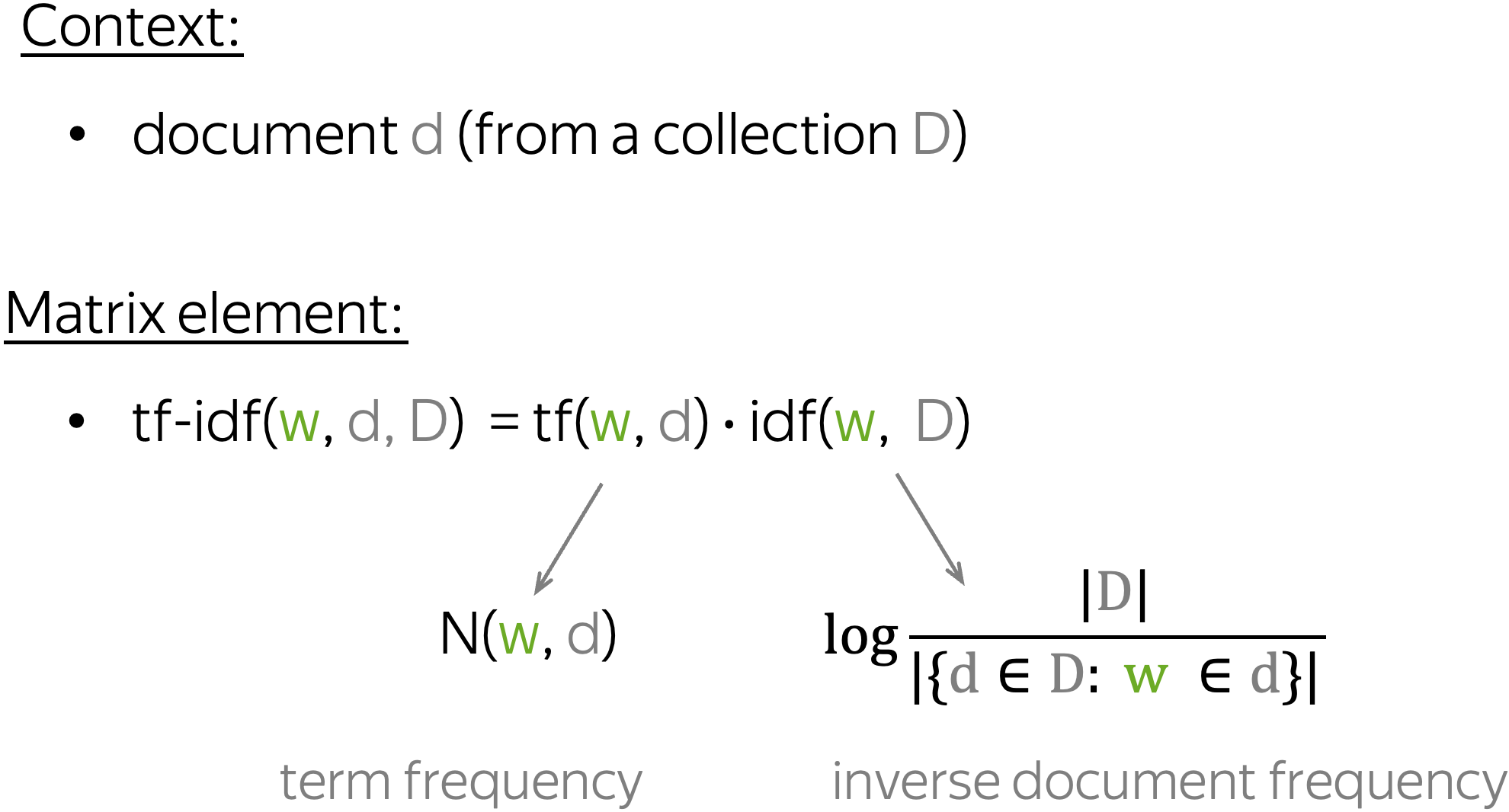
Latent Semantic Analysis (LSA) analyzes a collection of documents.
While in the previous approaches contexts served only to get word vectors
and were thrown away afterward, here we are also interested
in context, or, in this case, document vectors. LSA is one of the simplest topic models:
cosine similarity between document vectors can be used to measure similarity between documents.
The term «LSA» sometimes refers to a more general approach of applying SVD to a term-document
matrix where the term-document elements can be computed in different ways
(e.g., simple co-occurrence, tf-idf, or some other weighting).
Animation alert!
LSA wikipedia page has a nice
animation of the topic detection process in a document-word matrix — take a look!
Word2Vec: a Prediction-Based Method
Let us remember our main idea again:
Main idea:
We have to put information about contexts into word vectors.
While count-based methods took this idea quite literally, Word2Vec uses it in a different manner:
How:
Learn word vectors by teaching them to predict contexts.
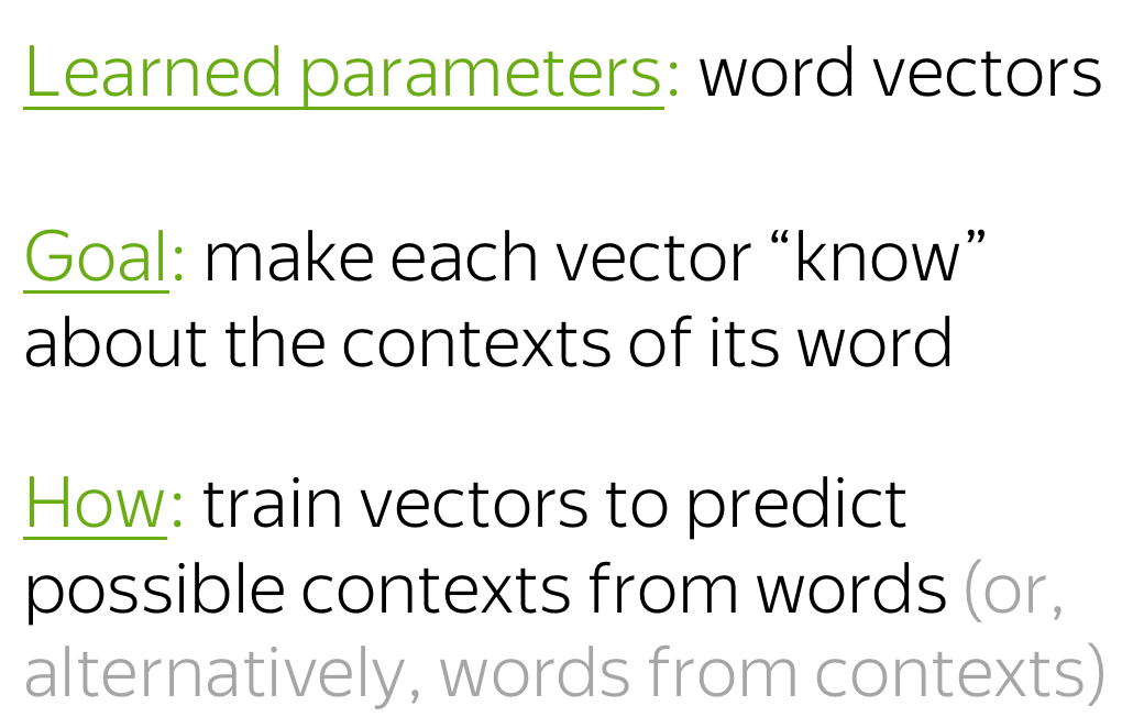
Word2Vec is a model whose parameters are word vectors. These parameters are optimized iteratively
for a certain objective. The objective forces word vectors to «know» contexts a word can appear in:
the vectors are trained to predict possible contexts of the corresponding words.
As you remember from the distributional hypothesis, if vectors «know» about contexts, they «know» word meaning.
Word2Vec is an iterative method. Its main idea is as follows:
- take a huge text corpus;
- go over the text with a sliding window, moving one word at a time. At each step, there is a central word
and context words (other words in this window); - for the central word, compute probabilities of context words;
- adjust the vectors to increase these probabilities.
![]()
![]()
Objective Function: Negative Log-Likelihood
For each position (t =1, dots, T) in a text corpus,
Word2Vec predicts context words within a m-sized window given the central
word (color{#88bd33}{w_t}):
[color{#88bd33}{mbox{Likelihood}} color{black}= L(theta)=
prodlimits_{t=1}^Tprodlimits_{-mle j le m, jneq 0}P(color{#888}{w_{t+j}}|color{#88bd33}{w_t}color{black}, theta), ]
where (theta) are all variables to be optimized.
The objective function (aka loss function or
cost function) (J(theta)) is the average negative log-likelihood:
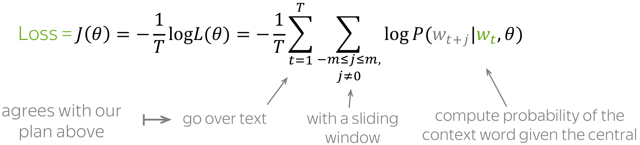
Note how well the loss agrees with our plan main above: go over text with a
sliding window and compute probabilities.
Now let’s find out how to compute these probabilities.
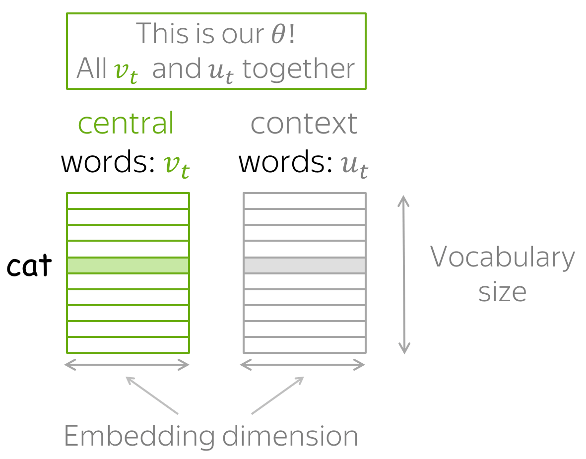
How to calculate (P(color{#888}{w_{t+j}}color{black}|color{#88bd33}{w_t}color{black}, theta))?
For each word (w) we will have two vectors:
- (color{#88bd33}{v_w}) when it is a central word;
- (color{#888}{u_w}) when it is a context word.
(Once the vectors are trained, usually we throw away context vectors and use
only word vectors.)
Then for the central word (color{#88bd33}{c}) (c — central) and
the context word (color{#888}{o}) (o — outside word)
probability of the context word is
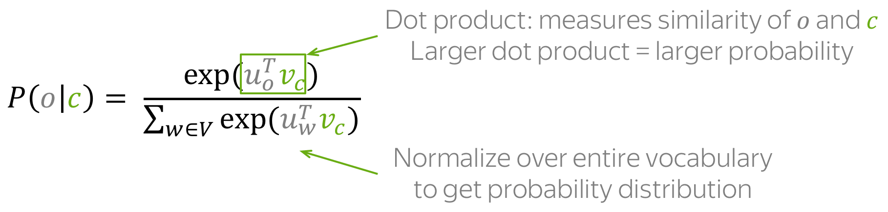
Note: this is the softmax function! (click for the details)
The function above is an example of the softmax function:
[softmax(x_i)=frac{exp(x_i)}{sumlimits_{j=i}^nexp(x_j)}.]
Softmax maps arbitrary values (x_i) to a probability
distribution (p_i):
- «max» because the largest (x_i) will have the largest probability (p_i);
- «soft» because all probabilities are non-zero.
You will deal with this function quite a lot over the NLP course (and in Deep Learning in general).
![]()
How to: go over the illustration. Note that for
central words and context words, different
vectors are used. For example, first the word a is central and
we use (color{#88bd33}{v_a}), but when it becomes context,
we use (color{#888}{u_a}) instead.
![]()
How to train: by Gradient Descent, One Word at a Time
Let us recall that our parameters (theta) are vectors (color{#88bd33}{v_w}) and (color{#888}{u_w})
for all words in the vocabulary. These vectors are learned by optimizing the training objective via gradient descent
(with some learning rate (alpha)):
[theta^{new} = theta^{old} — alpha nabla_{theta} J(theta).]
One word at a time
We make these updates one at a time: each update is for
a single pair of a center word and one of its context words.
Look again at the loss function:
[color{#88bd33}{mbox{Loss}}color{black} =J(theta)= -frac{1}{T}log L(theta)=
-frac{1}{T}sumlimits_{t=1}^T
sumlimits_{-mle j le m, jneq 0}log P(color{#888}{w_{t+j}}color{black}|color{#88bd33}{w_t}color{black}, theta)=
frac{1}{T} sumlimits_{t=1}^T
sumlimits_{-mle j le m, jneq 0} J_{t,j}(theta). ]
For the center word (color{#88bd33}{w_t}), the loss contains a distinct term
(J_{t,j}(theta)=-log P(color{#888}{w_{t+j}}color{black}|color{#88bd33}{w_t}color{black}, theta)) for each of its context words
(color{#888}{w_{t+j}}).
Let us look in more detail at just this one term and try to understand how to make an update for this step. For example,
let’s imagine we have a sentence

with the central word cat,
and four context words.
Since we are going to look at just one step, we will pick only one of the context words; for example, let’s take
cute.
Then
the loss term for the central word cat
and the context word cute is:
[ J_{t,j}(theta)= -log P(color{#888}{cute}color{black}|color{#88bd33}{cat}color{black}) =
-log frac{expcolor{#888}{u_{cute}^T}color{#88bd33}{v_{cat}}}{
sumlimits_{win Voc}exp{color{#888}{u_w^T}color{#88bd33}{v_{cat}} }} =
-color{#888}{u_{cute}^T}color{#88bd33}{v_{cat}}color{black}
+ log sumlimits_{win Voc}exp{color{#888}{u_w^T}color{#88bd33}{v_{cat}}}color{black}{.}
]
Note which parameters are present at this step:
- from vectors for central words, only (color{#88bd33}{v_{cat}});
- from vectors for context words, all (color{#888}{u_w}) (for all words in
the vocabulary).
Only these parameters will be updated at the current step.
Below is the schematic illustration of
the derivations for this step.
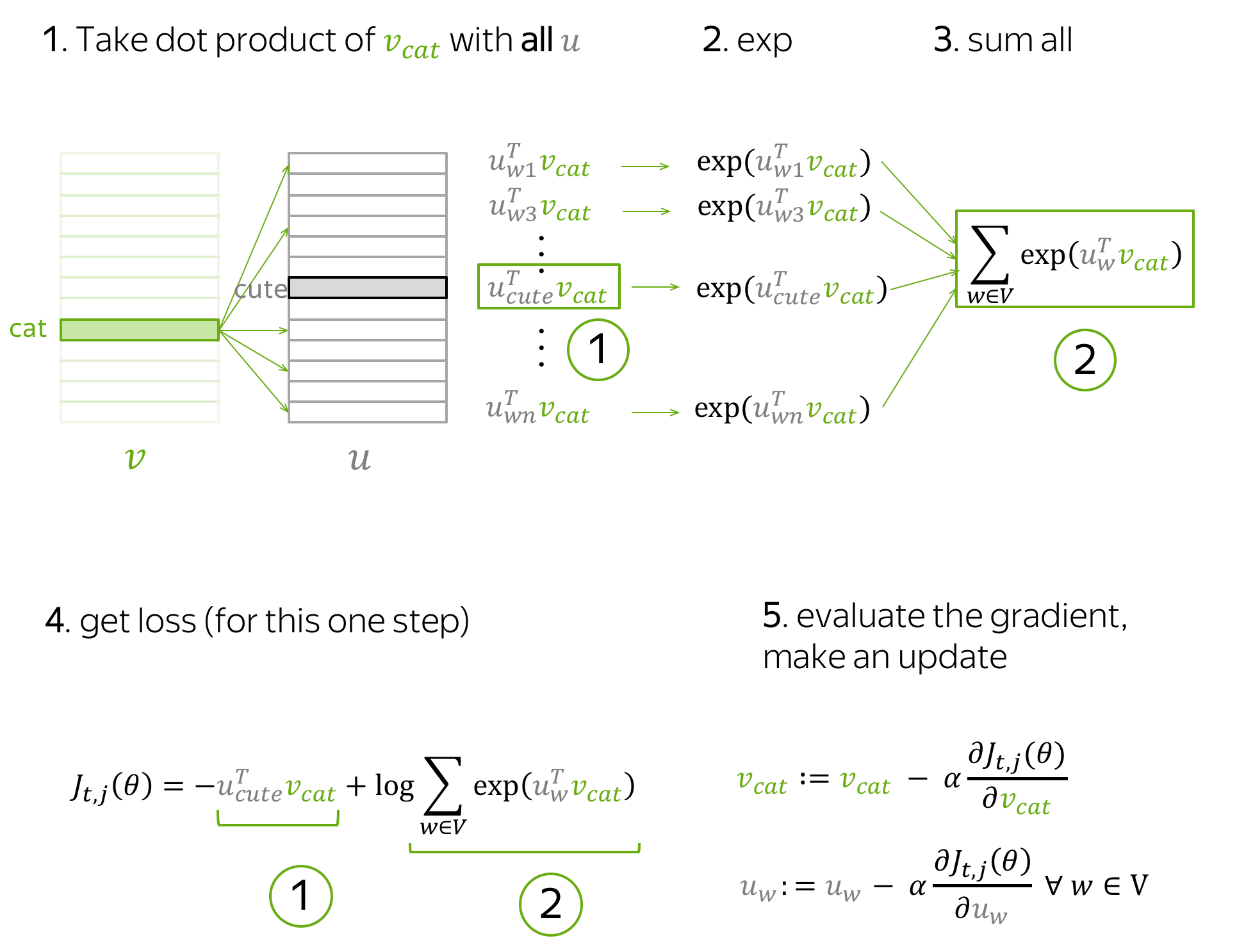
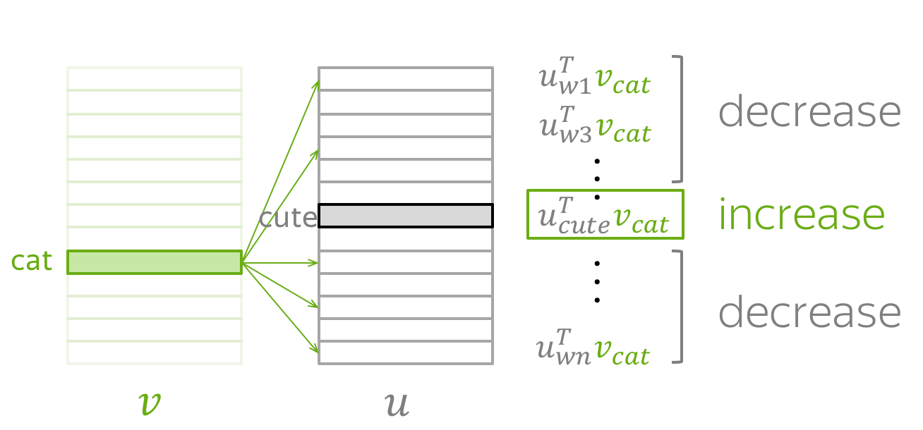
By making an update to minimize (J_{t,j}(theta)), we force the parameters to
increase similarity (dot product)
of (color{#88bd33}{v_{cat}}) and (color{#888}{u_{cute}}) and, at the same time,
to decrease
similarity between (color{#88bd33}{v_{cat}}) and (color{#888}{u_{w}}) for all other words (w) in the vocabulary.
This may sound a bit strange: why do we want to decrease similarity between (color{#88bd33}{v_{cat}})
and all other words, if some of them are also valid context words (e.g.,
grey,
playing,
in on our example sentence)?
But do not worry: since we make updates for each context word (and for all central words in your text),
on average over all updates
our vectors will learn
the distribution of the possible contexts.
Faster Training: Negative Sampling
In the example above, for each pair of a central word and its context word, we had to update all vectors
for context words. This is highly inefficient: for each step, the time needed to make an update is proportional
to the vocabulary size.
But why do we have to consider all context vectors in the vocabulary at each step?
For example, imagine that at the current step we consider context vectors not for all words,
but only for the current target (cute)
and several randomly chosen words. The figure shows the intuition.
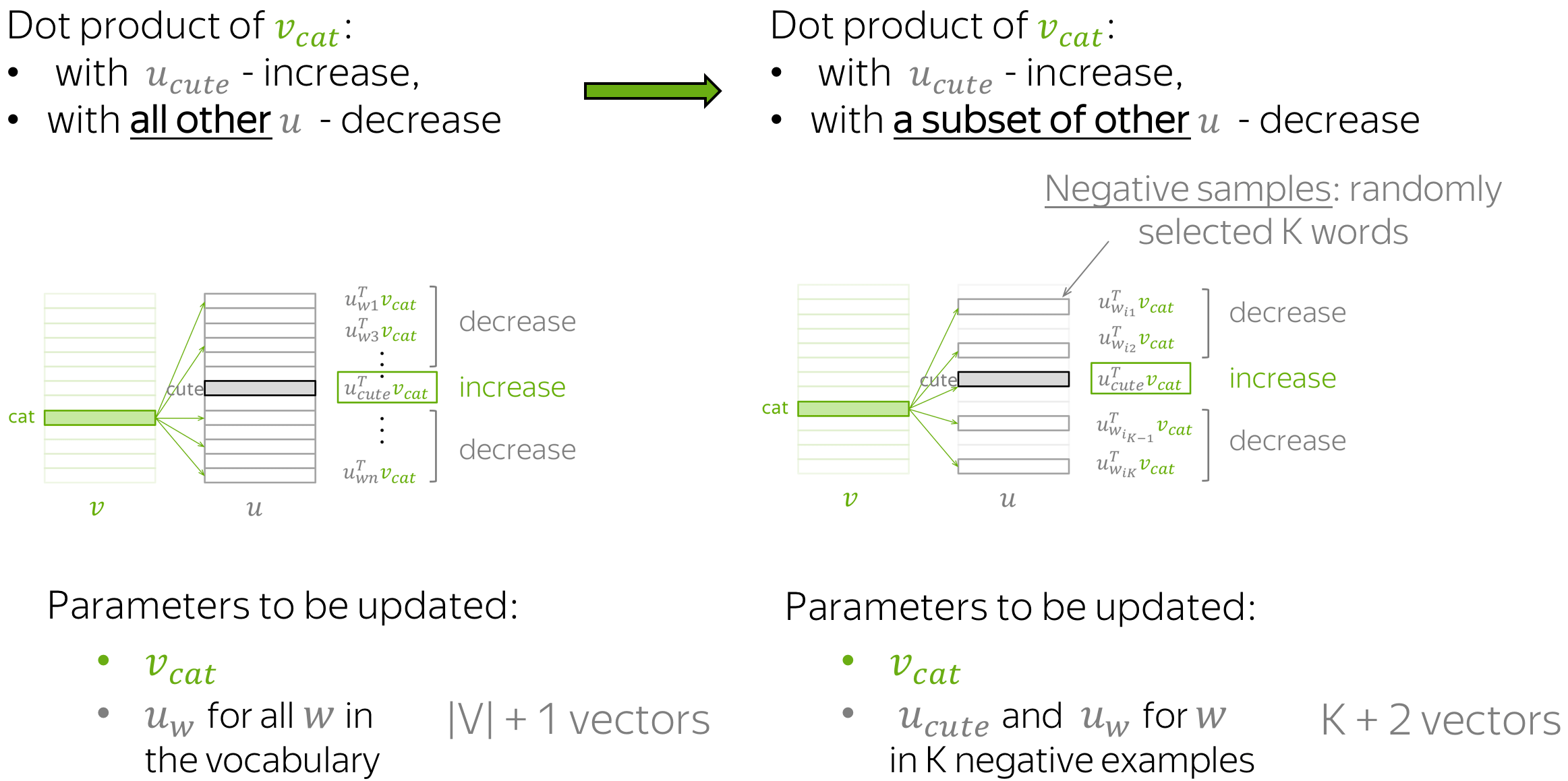
As before, we are increasing similarity between
(color{#88bd33}{v_{cat}}) and (color{#888}{u_{cute}}). What is different, is that now we
decrease similarity between (color{#88bd33}{v_{cat}}) and context vectors not for all words, but only
with a subset of K «negative» examples.
Since we have a large corpus, on average over all updates we will update each vector sufficient number of times,
and the vectors will still be able to learn the relationships between words quite well.
Formally, the new loss function for this step is:
[ J_{t,j}(theta)=
-logsigma(color{#888}{u_{cute}^T}color{#88bd33}{v_{cat}}color{black}) —
sumlimits_{win {w_{i_1},dots, w_{i_K}}}logsigma({-color{#888}{u_w^T}color{#88bd33}{v_{cat}}}color{black}),
]
where (w_{i_1},dots, w_{i_K}) are the K negative examples chosen at this step
and (sigma(x)=frac{1}{1+e^{-x}}) is the sigmoid function.
Note that
(sigma(-x)=frac{1}{1+e^{x}}=frac{1cdot e^{-x}}{(1+e^{x})cdot e^{-x}} =
frac{e^{-x}}{1+e^{-x}}= 1- frac{1}{1+e^{x}}=1-sigma(x)). Then the loss can also be written as:
[ J_{t,j}(theta)=
-logsigma(color{#888}{u_{cute}^T}color{#88bd33}{v_{cat}}color{black}) —
sumlimits_{win {w_{i_1},dots, w_{i_K}}}log(1-sigma({color{#888}{u_w^T}color{#88bd33}{v_{cat}}}color{black})).
]
![]()
How the gradients and updates change when using negative sampling?
The Choice of Negative Examples
Each word has only a few «true» contexts. Therefore, randomly chosen words are very likely to be «negative», i.e. not
true contexts. This simple idea is used not only to train Word2Vec efficiently but also in many other
applications, some of which we will see later in the course.
Word2Vec randomly samples negative examples based on the empirical distribution of words.
Let (U(w)) be a unigram distribution of words, i.e. (U(w)) is the frequency of the word (w)
in the text corpus. Word2Vec modifies this distribution to sample less frequent words more often:
it samples proportionally to (U^{3/4}(w)).
Word2Vec variants: Skip-Gram and CBOW
There are two Word2Vec variants: Skip-Gram and CBOW.
Skip-Gram is the model we considered so far: it predicts context words given the central word.
Skip-Gram with negative sampling is the most popular approach.
CBOW (Continuous Bag-of-Words) predicts the central word from the sum of context vectors. This simple sum of
word vectors is called «bag of words», which gives the name for the model.
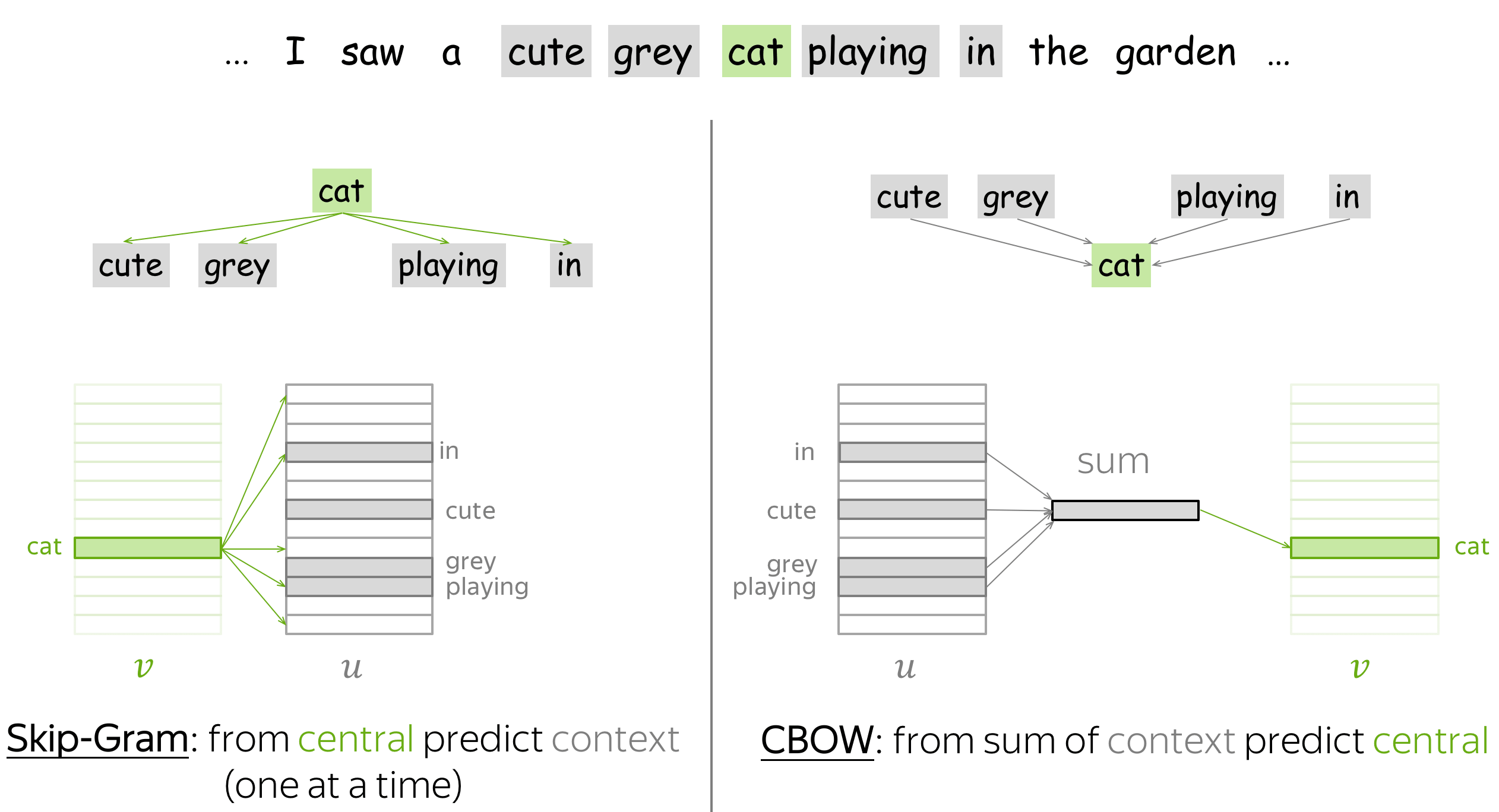
Additional Notes
The original Word2Vec papers are:
- Efficient Estimation of Word Representations in Vector Space
- Distributed Representations of Words and Phrases and their Compositionality
You can look into them for the details on the experiments, implementation and hyperparameters. Here we will
provide some of the most important things you need to know.
The Idea is Not New
The idea to learn word vectors (distributed representations) is not new. For example, there were attempts to
learn word vectors as part of a larger network and then extract the embedding layer. (For the details on the
previous methods, you can look, for example, at the summary in the original Word2Vec papers).
What was very unexpected in Word2Vec, is its ability to learn high-quality word vectors
very fast on huge datasets and for
large vocabularies. And of course, all the fun properties we will see in the
Analysis and Interpretability section quickly made Word2Vec very famous.
Why Two Vectors?
As you remember, in Word2Vec we train two vectors for each word: one when it is a central word and another
when it is a context word. After training, context vectors are thrown away.
This is one of the tricks that made Word2Vec so simple. Look again at the loss function (for one step):
[ J_{t,j}(theta)=
-color{#888}{u_{cute}^T}color{#88bd33}{v_{cat}}color{black} —
log sumlimits_{win V}exp{color{#888}{u_w^T}color{#88bd33}{v_{cat}}}color{black}{.}
]
When central and context words have different vectors, both the first term and dot products inside the exponents
are linear with respect to the parameters (the same for the negative training objective).
Therefore, the gradients are easy to compute.
![]()
Repeat the derivations (loss and the gradients) for the case with one vector for each word
((forall w in V, color{#88bd33}{v_{w}}color{black}{ = }color{#888}{u_{w}}) ).
![]()
While the standard practice is to throw away context vectors, it was shown that
averaging word and context vectors may be more beneficial.
More details are here.
Better training
![]()
There’s one more trick: learn more from this exercise
in the Research Thinking section.
Relation to PMI Matrix Factorization
![]()
Word2Vec SGNS (Skip-Gram with Negative Sampling)
implicitly approximates the factorization of a (shifted) PMI matrix.
Learn more here.
The Effect of Window Size
The size of the sliding window has a strong effect on the resulting
vector similarities.
For example, this paper notes that
larger windows tend to produce more topical similarities
(i.e. dog,
bark and
leash will be grouped together,
as well as
walked,
run and
walking),
while smaller windows tend to produce more functional and syntactic similarities
(i.e. Poodle,
Pitbull,
Rottweiler, or
walking,
running,
approaching).
(Somewhat) Standard Hyperparameters
As always, the choice of hyperparameters usually depends on the task at hand;
you can look at the original papers for more details.
Somewhat standard setting is:
- Model: Skip-Gram with negative sampling;
- Number of negative examples: for smaller datasets, 15-20; for huge datasets
(which are usually used) it can be 2-5. - Embedding dimensionality: frequently used value is 300, but other
variants (e.g., 100 or 50) are also possible. For theoretical explanation of the optimal dimensionality,
take a look at the Related Papers section. - Sliding window (context) size: 5-10.
GloVe: Global Vectors for Word Representation
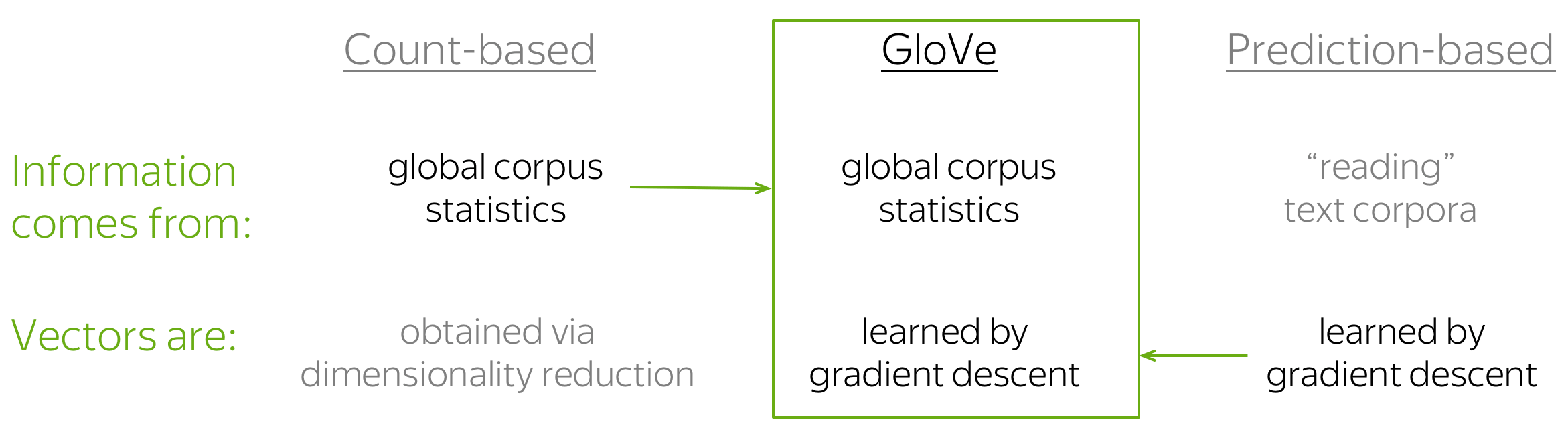
The GloVe model is a combination of
count-based methods and prediction methods (e.g., Word2Vec). Model name, GloVe, stands
for «Global Vectors», which reflects its idea: the method uses
global information from corpus to learn vectors.
As we saw earlier, the simplest count-based method uses
co-occurrence counts to measure the association between word
w
and context c:
N(w, c).
GloVe also uses these counts to construct the loss function:
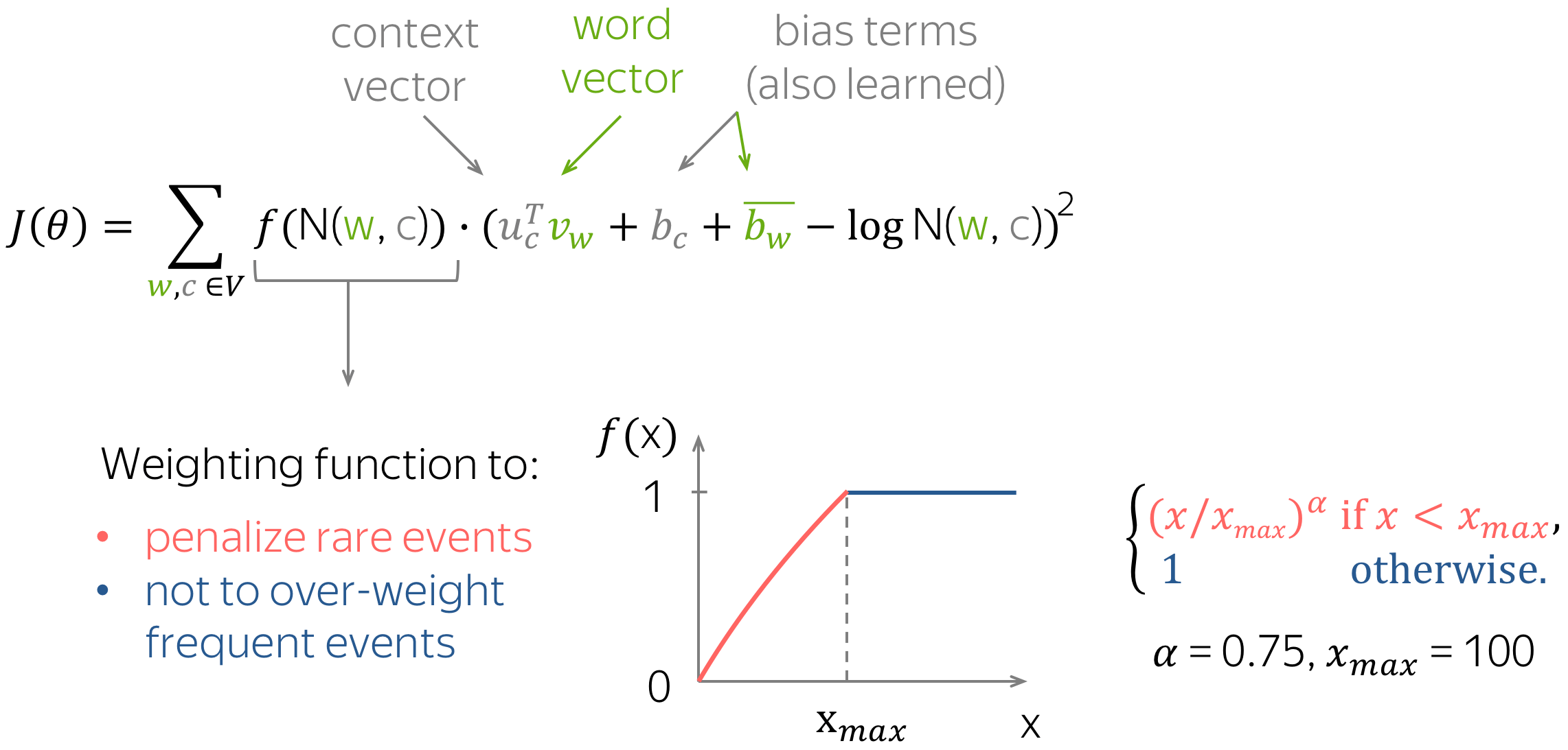
Similar to Word2Vec, we also have different vectors for
central and context words — these are our parameters.
Additionally, the method has a scalar bias term for each word vector.
What is especially interesting, is the way GloVe controls the influence of rare and frequent words:
loss for each pair (w, c) is weighted in a way that
- rare events are penalized,
- very frequent events are not over-weighted.
Lena:
The loss function looks reasonable as it is, but
the original GloVe paper
has very nice motivation leading to the above formula. I will not provide it here
(I have to finish the lecture at some point, right?..), but
you can read it yourself — it’s really, really nice!
Evaluation of Word Embeddings
How can we understand that one method for getting word embeddings is better than another?
There are two types of evaluation (not only for word embeddings): intrinsic and extrinsic.
Intrinsic Evaluation: Based on Internal Properties
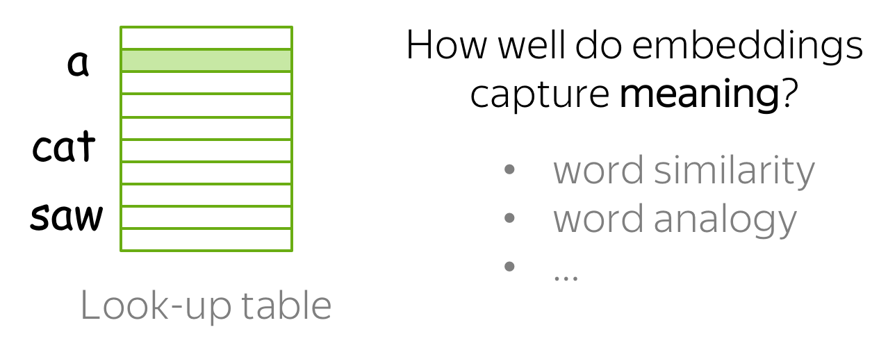
This type of evaluation looks at the internal properties of embeddings, i.e.
how well they capture meaning. Specifically, in the
Analysis and Interpretability section,
we will discuss in detail how we can evaluate embeddings on word similarity and word analogy tasks.
Extrinsic Evaluation: On a Real Task
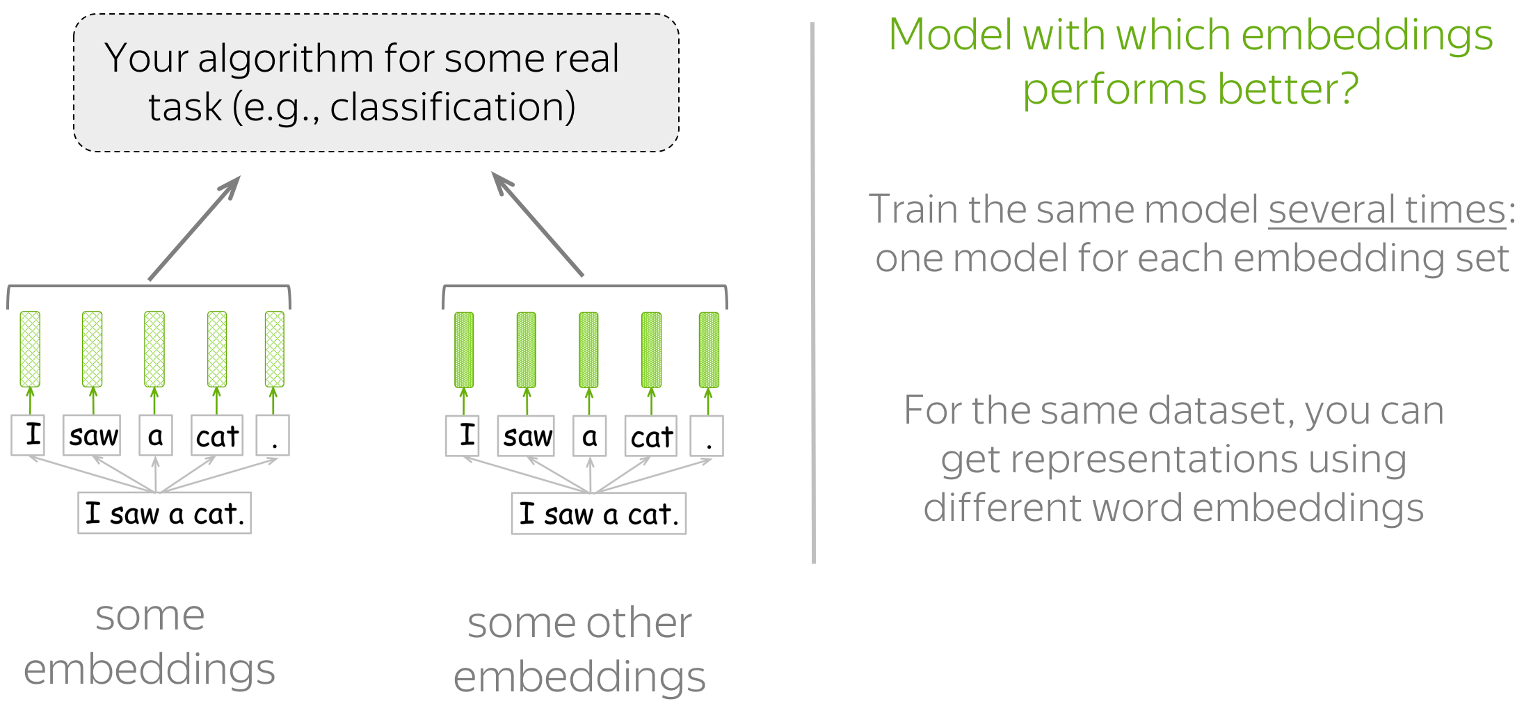
This type of evaluation tells which embeddings are better for the task you really care about (e.g.,
text classification, coreference resolution, etc.).
In this setting, you have to train the model/algorithm for the real task several times: one model for each of the
embeddings you want to evaluate. Then, look at the quality of these models to decide which
embeddings are better.
How to Choose?
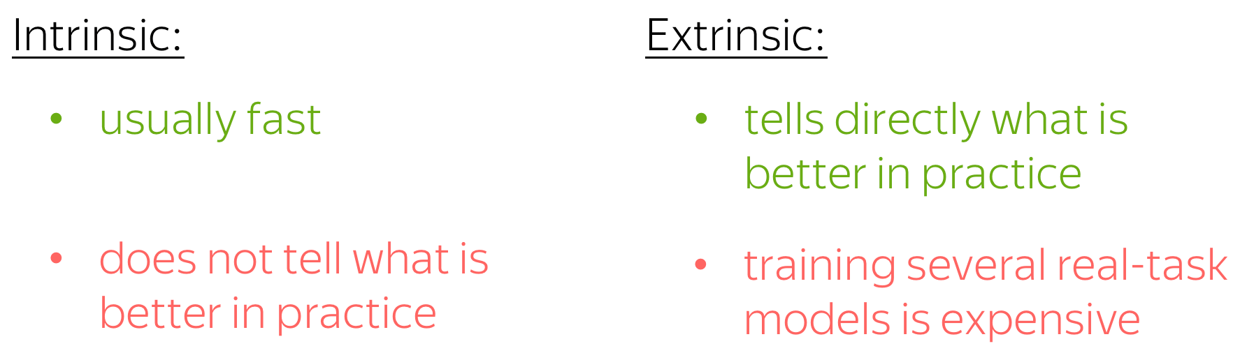
One thing you have to get used to is that there is no perfect solution and no right answer
for all situations: it always depends on many things.
Regarding evaluation, you usually care about quality of the task you want to solve. Therefore,
you are likely to be more interested in extrinsic evaluation. However, real-task models
usually require a lot of time and resources to train, and training several of them may
be too expensive.
In the end, this is your call to make 
![]()
Analysis and Interpretability
Lena: For word embeddings, most of the content of
this part is usually considered as evaluation (intrinsic evaluation). However,
since looking at what a model learned (beyond task-specific metrics) is the kind of thing
people usually do for analysis, I believe it can be presented here, in the analysis section.
Take a Walk Through Space… Semantic Space!
Semantic spaces aim to create representations of natural language that capture meaning.
We can say that (good) word embeddings form semantic space and will refer to
a set of word vectors in a multi-dimensional space as «semantic space».
Below is shown semantic space formed by GloVe vectors trained on twitter data (taken from
gensim). Vectors were
projected to two-dimensional space using t-SNE; these are only the top-3k most frequent words.
![]()
How to: Walk through semantic space and try to find:
- language clusters: Spanish, Arabic, Russian, English. Can you find more languages?
- clusters for: food, family, names, geographical locations. What else can you find?
![]()
Nearest Neighbors
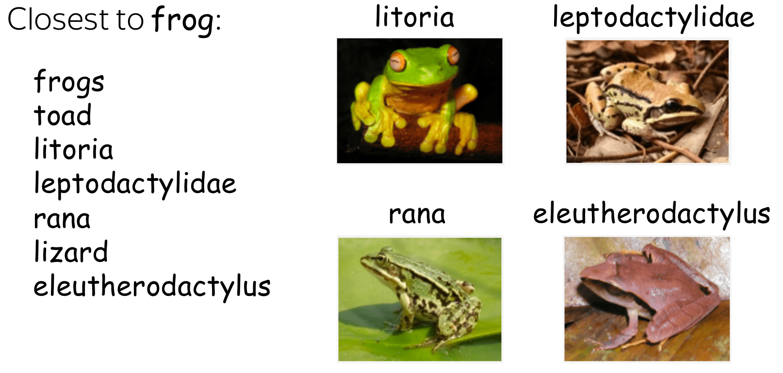
The example is
from the GloVe project page.
During your walk through semantic space, you probably noticed that the points (vectors) which are nearby
usually have close meaning. Sometimes, even rare words are understood very well. Look at the example:
the model understood that words such as leptodactylidae
or litoria are close to
frog.
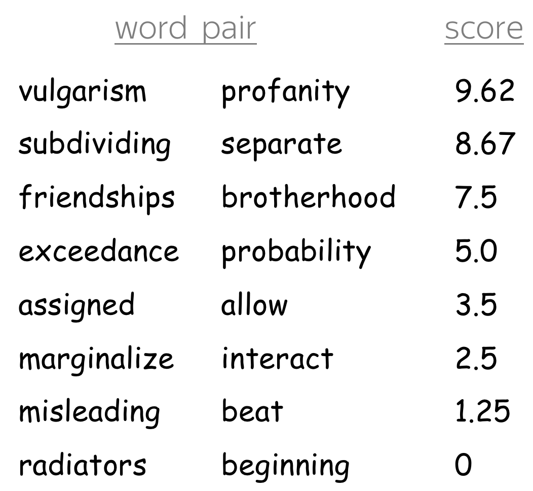
Several pairs from the
Rare Words similarity benchmark.
Word Similarity Benchmarks
«Looking» at nearest neighbors (by cosine similarity or Euclidean distance) is one of the
methods to estimate the quality of the learned embeddings. There are several
word similarity benchmarks (test sets). They consist
of word pairs with a similarity score according to human judgments.
The quality of embeddings is estimated as
the correlation between the two similarity scores (from model and from humans).
Linear Structure
While similarity results are encouraging, they are not surprising: all in all,
the embeddings were trained specifically to reflect word similarity.
What is surprising, is that many semantic and syntactic relationships between words
are (almost) linear in word vector space.
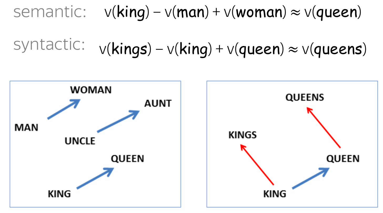
For example, the difference between
king and
queen
is (almost) the same as between
man
and woman.
Or a word that is similar to
queen
in the same sense that
kings is similar to
king turns out to be
queens.
The
man-woman (approx)
king-queen example
is probably the most popular one, but there are also many other relations and funny examples.
Below are examples for the country-capital relation
and a couple of syntactic relations.
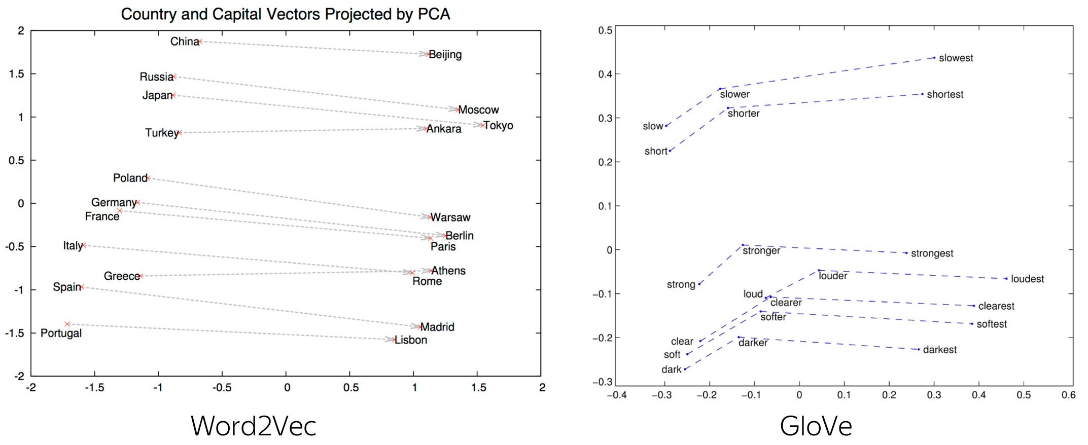
![]()
At ICML 2019, it was shown that there’s actually a theoretical explanation for
analogies in Word2Vec.
More details are here.
Lena: This paper,
Analogies Explained: Towards Understanding Word Embeddings
by Carl Allen and Timothy Hospedales from the University of Edinburgh, received
Best Paper Honourable Mention award at ICML 2019 — well deserved!
Word Analogy Benchmarks
These near-linear relationships inspired a new type of evaluation:
word analogy evaluation.
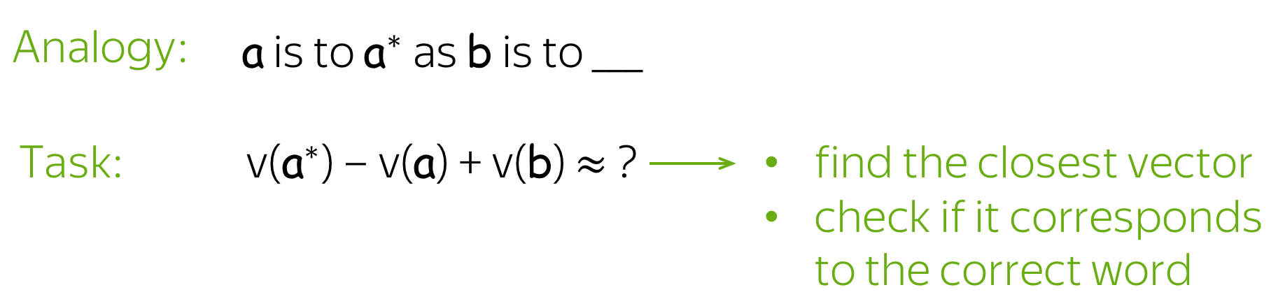
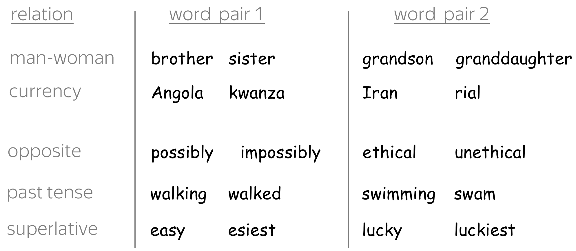
Examples of relations and word pairs from
the Google analogy test set.
Given two word pairs for the same relation, for example
(man, woman) and
(king, queen),
the task is to check if we can identify one of the words based on the rest of them.
Specifically, we have to check if the closest vector to
king — man + woman
corresponds to the word
queen.
Now there are several analogy benchmarks; these include
the standard benchmarks (MSR +
Google analogy test sets) and
BATS (the Bigger Analogy Test Set).
Similarities across Languages
We just saw that some relationships between words are (almost) linear in the embedding space.
But what happens across languages? Turns out, relationships between semantic spaces are also
(somewhat) linear: you can linearly map one semantic space to another so that
corresponding words in the two languages match in the new, joint semantic space.
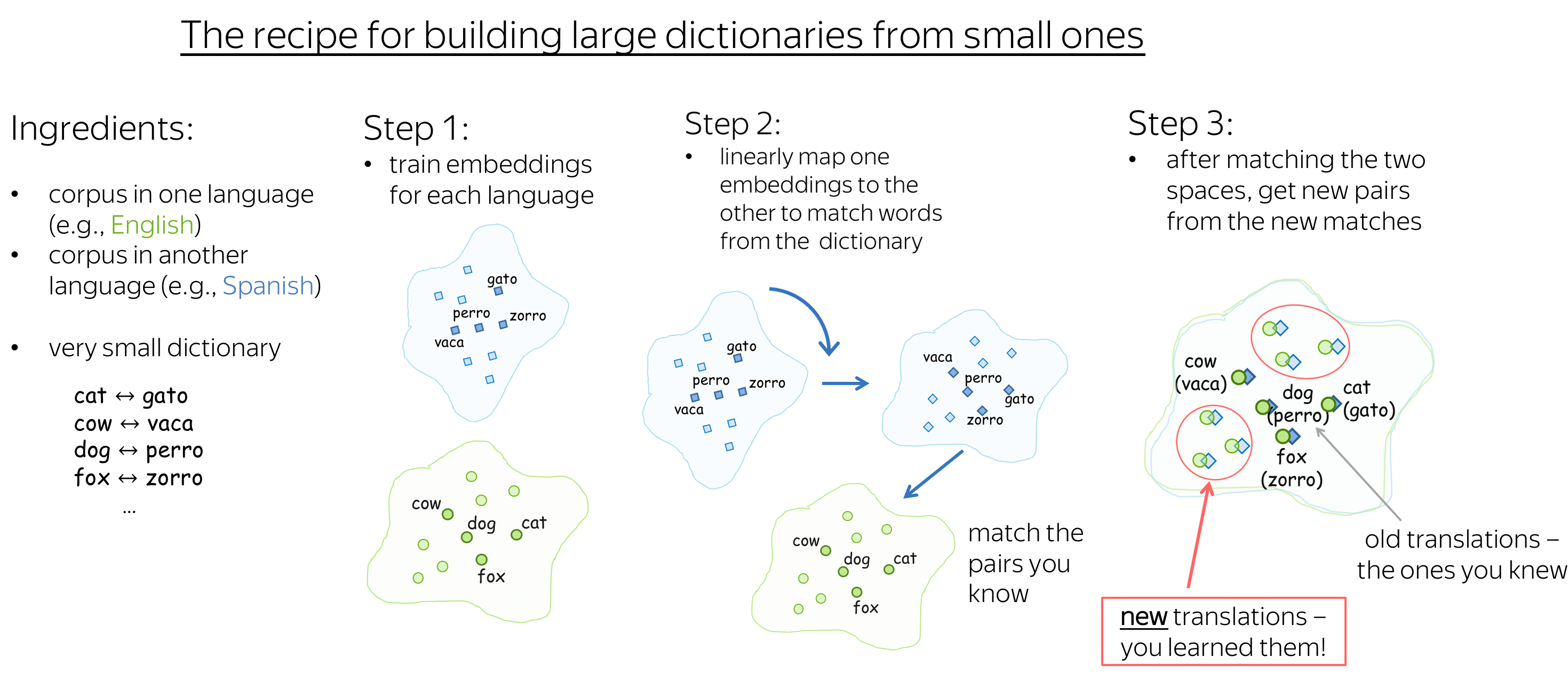
The figure above illustrates the approach proposed
by Tomas Mikolov et al. in 2013 not long after the original Word2Vec. Formally,
we are given a set of word pairs and their vector representations
({color{#88a635}{x_i}color{black}, color{#547dbf}{z_i}color{black} }_{i=1}^n),
where (color{#88a635}{x_i}) and (color{#547dbf}{z_i})
are vectors for i-th word in the source language and its translation in the target.
We want to find a transformation matrix W such that (Wcolor{#547dbf}{z_i}) approximates (color{#88a635}{x_i})
: «matches» words from the dictionary.
We pick (W) such that
[W = arg minlimits_{W}sumlimits_{i=1}^nparallel Wcolor{#547dbf}{z_i}color{black} — color{#88a635}{x_i}color{black}parallel^2,]
and learn this matrix by gradient descent.
In the original paper, the initial vocabulary consists of the 5k most frequent words with their translations,
and the rest is learned.
![]()
Later it turned out, that we don’t need a dictionary at all —
we can build a mapping between semantic spaces even
if we know nothing about languages! More details are
here.
![]()
Is the «true» mapping between languages indeed linear, or more complicated?
We can look at geometry of the learned semantic spaces and check.
More details are
here.
![]()
The idea to linearly map different embedding sets to (nearly) match them can also be used
for a very different task!
Learn more
in the Research Thinking section.
![]()
Research Thinking
How to
- Read the short description at the beginning — this is our starting point,
something known. - Read a question and think: for a minute, a day, a week, … —
give yourself some time! Even if you are not thinking about it constantly,
something can still come to mind. - Look at the possible answers — previous attempts to answer/solve this problem.
Important:
You are not supposed to come up with
something exactly like here — remember, each paper usually takes the authors several
months of work. It’s a habit of thinking about these things that counts!
All the rest a scientist needs is time: to try-fail-think
until it works.
It’s well-known that you will learn something easier if you are not just given the answer right away,
but if you think about it first. Even if you don’t want to be a researcher, this is still a good way
to learn things!
Count-Based Methods
Improve Simple Co-Occurrence Counts
The simplest co-occurrence counts treat context words equally, although these words
are at different relative positions from the central word.
For example, from one sentence
the central word cat
will get a co-occurrence count of 1 for each of the words
cute,
grey,
playing,
in (look at the example to the right).
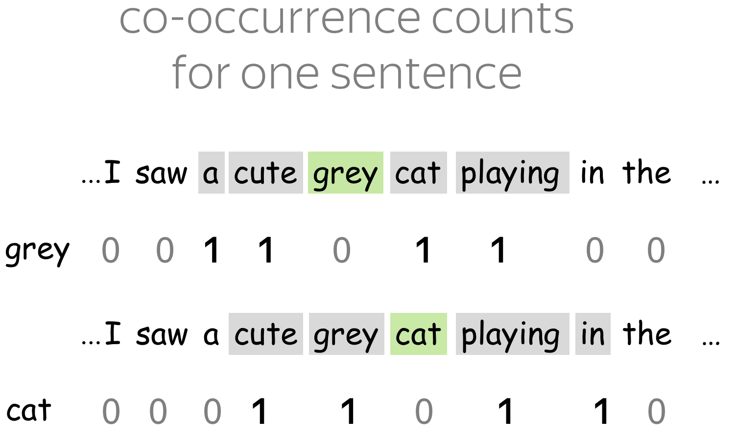
?
Are context words at different distances equally important?
If not, how can we modify co-occurrence counts?
Possible answers
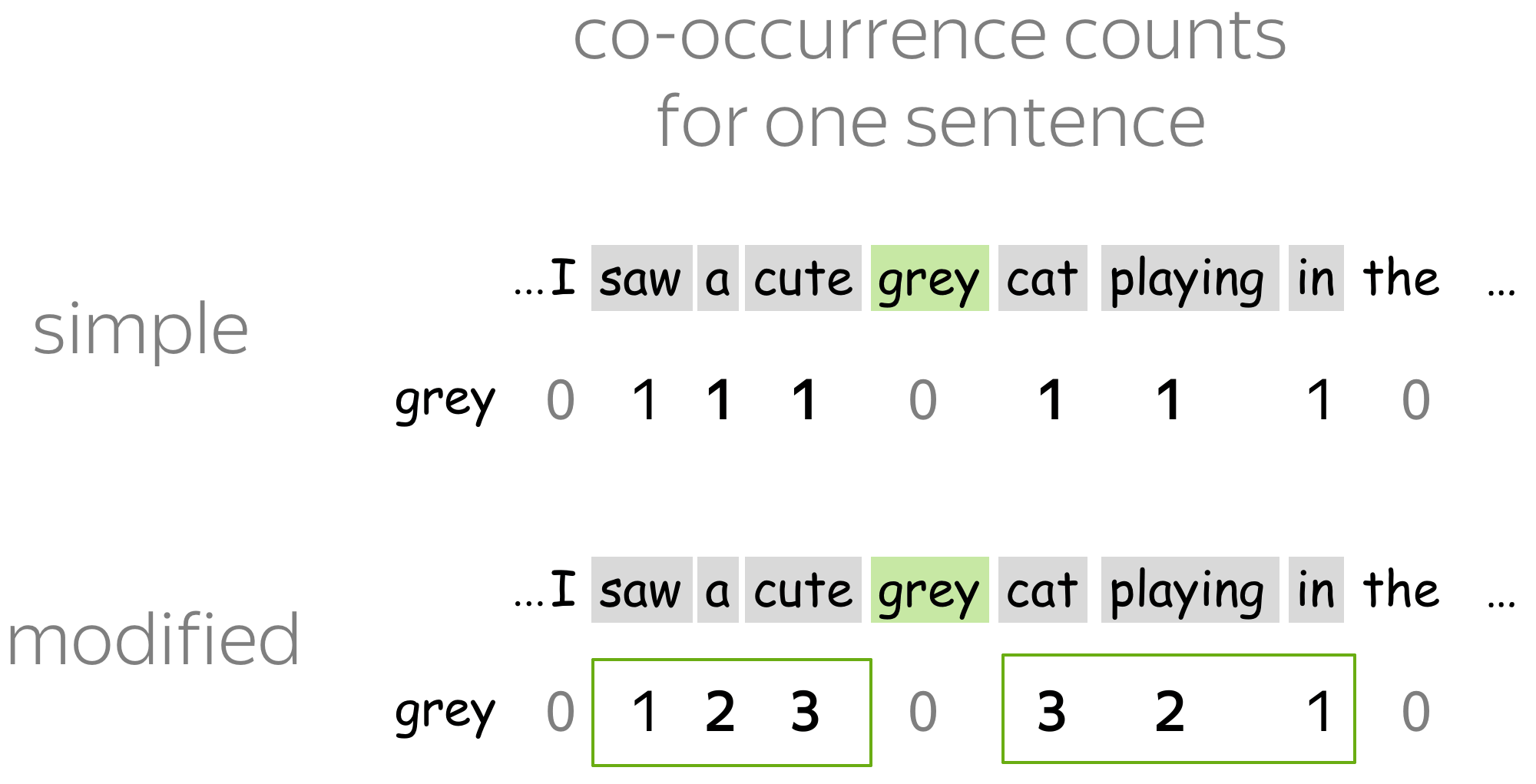
Intuitively, words that are closer to the central are more important; for example,
immediate neighbors are more informative than words at distance 3.
We can use this to modify the model: when evaluating counts,
let’s give closer words more weight. This idea was used in the
HAL model (1996),
which once was very famous. They modified counts as shown in the example.
?
In language, word order is important; specifically, left and right contexts have different meanings.
How can we distinguish between the left and right contexts?
One of the existing approaches
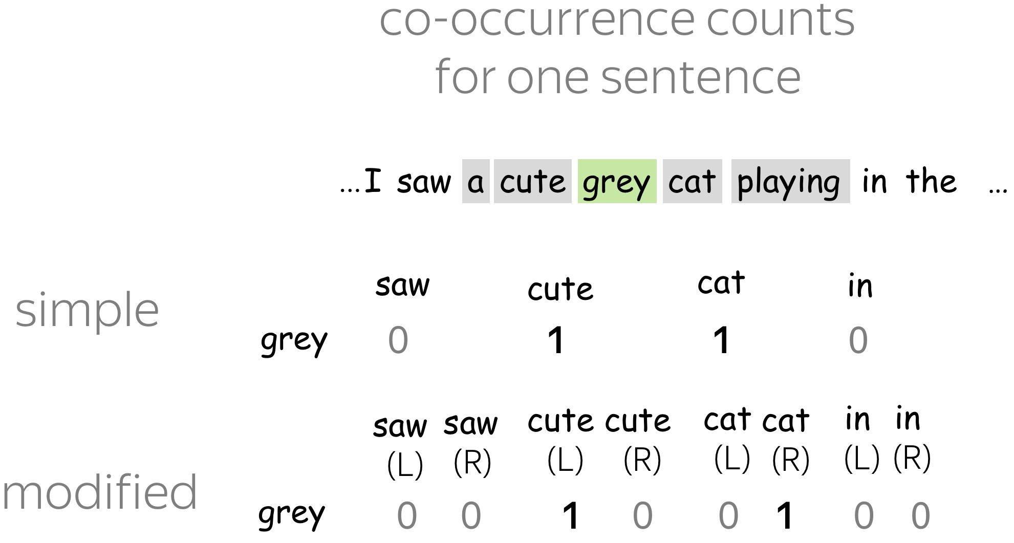
Here the weighting idea we saw above would not work: we can not say which
contexts, left or right, are more important.
What we have to do is to evaluate co-occurrences to the left and to the right separately.
For each context word, we will have two different counts: one when it is a left context and
another when it is the right context. This means that our co-occurrence matrix will have
|V| rows and 2|V| columns.
This idea was also used in the
HAL model (1996).
Look at the example; note that for cute,
we have left co-occurrence count, for
cat — right.
Word2Vec
Are all context words equally important for training?
During Word2Vec training, we make an update for each of the context words.
For example, for the central word cat
we make an update for each of the words
cute,
grey,
playing,
in.
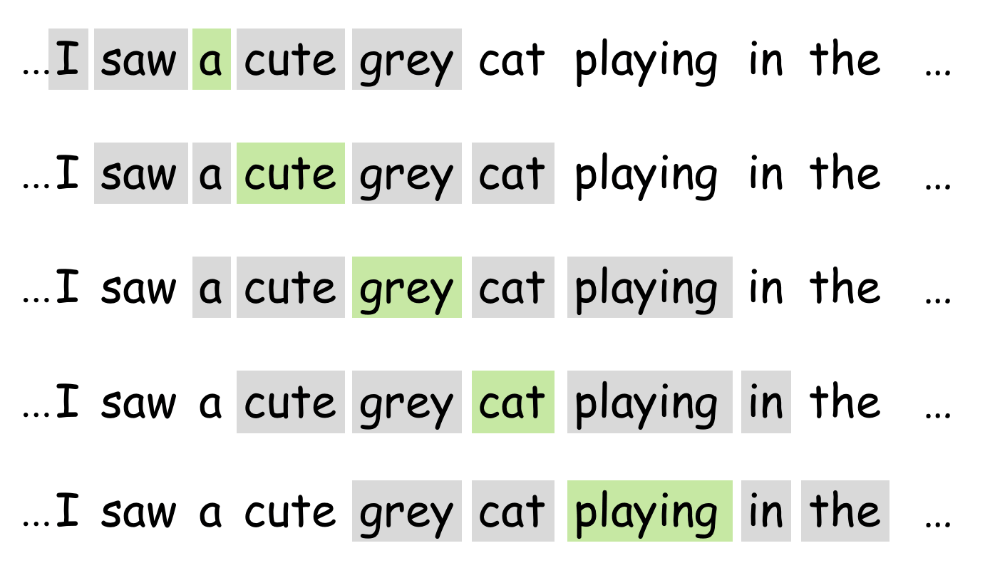
?
Are all context words equally important?
Which word types give more/less information than others?
Think about some characteristics of words
that can influence their importance. Do not forget the previous exercise!
Possible answers
- word frequency
We can expect that frequent words usually give less information than rare ones.
For example, the fact that cat
appears in context of in
does not tell us much about the meaning of
cat: the word
in serves as a context for many other words.
In contrast,
cute,
grey and
playing
already give us some idea about
cat. -
distance from the central word
As we discussed in the previous exercise
on count-based methods, words that are closer to the central may be more important.
?
How can we use this to modify training?
Tricks from the original Word2Vec
1. Word Frequency

To account for different informativeness of rare and frequent words,
Word2Vec uses a simple subsampling
approach: each word (w_i) in the training set is ignored with probability
computed by the formula
[P(w_i)=1 — sqrt{frac{thr}{f(w_i)}}]
where (f(w_i)) is the word frequency and (thr) is the chosen threshold
(in the original paper, (thr=10^{-5})).
This formula preserves the ranking of the frequencies, but aggressively subsamples words whose
frequency is greater than (thr).
Interestingly, this heuristic
works well in practice:
it accelerates learning and even significantly improves the
accuracy of the learned vectors of the rare words.
2. Distance from the central word
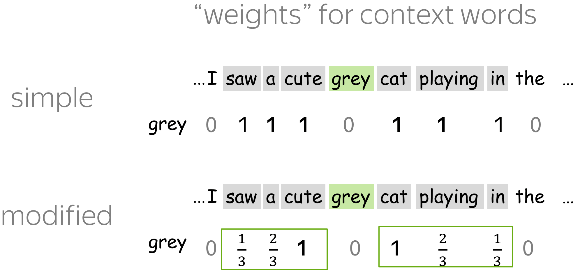
As in the previous exercise
on count-based methods, we can assign higher weights to the words which are closer to
the central.
At the first glance, you won’t see any weights in the original Word2Vec implementation.
However, at each step it samples the size of the context window from 1 to L. Therefore,
words which are closer to central are used more frequently than the distant ones.
In the original work this was (probably) done for efficiency (fewer updates for each step),
but this also has the effect similar to assigning weights.
Use Information About Subwords («invent» FastText)
Usually, we have a look-up table where each word is assigned a distinct vector.
By construction, these vectors do not have any idea about subwords they consist of:
all information they have is what they learned from contexts.
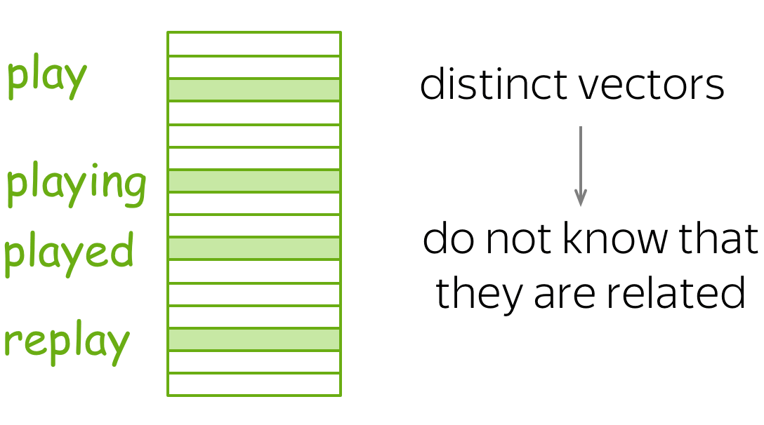
?
Imagine that word embeddings have some understanding of subwords they consist of.
Why can this be useful?
Possible answers
- better understanding of morphology
By assigning a distinct vector to each word, we ignore morphology. Giving information about
subwords can let the model know that different tokens can be forms of the same word. - representations for unknown words
Usually, we can represent only those words, which are present in the vocabulary.
Giving information about
subwords can help to represent out-of-vocabulary words relying of their spelling. - handling misspellings
Even if one character in a word is wrong, this is another token, and,
therefore, a completely different embedding
(or even unknown word). With information about subwords, misspelled word would still
be similar to the original one.
?
How can we incorporate information about subwords into embeddings? Let’s assume that the training pipeline
is fixed, e.g., Skip-Gram with Negative sampling.
One of the existing approaches (FastText)
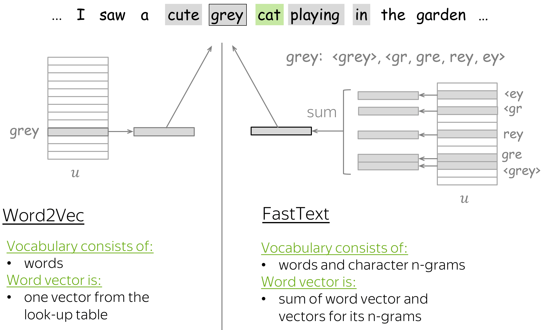
One of the possible approaches is to compose a word vector from vectors for its subwords.
For example, popular
FastText embeddings
operate as shown in the illustration. For each word, they add special start and end
characters for each word. Then, in addition to the vector for this word, they also use vectors
for character n-grams (which are also in the vocabulary). Representation of a word
us sum of vectors for the word and its subwords, as shown in the picture.
Note that this changes only the way we form word vector; the whole training pipeline is the same
as in the standard Word2Vec.
Semantic Change
Detect Words that Changed Their Usage
Imagine you have text corpora from different sources:
time periods, populations, geographic regions, etc.
In digital humanities and computational social science, people
often want to find words that used differently in these corpora.
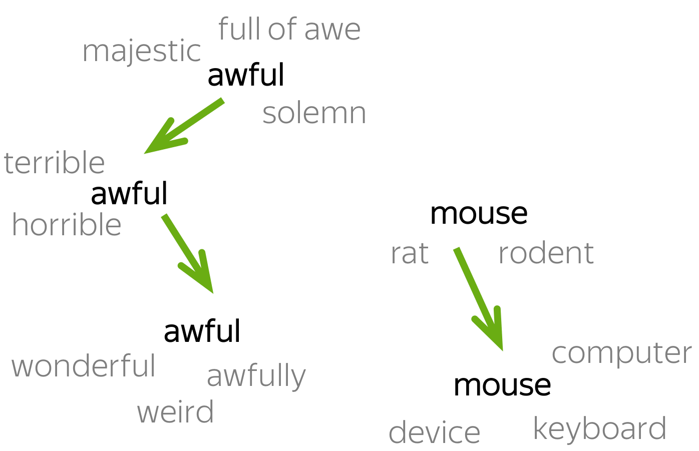
?
Given two text corpora, how would you detect which words are used differently/have different meaning?
Do not be shy to think about very simple ways!
Some of the existing attempts
ACL 2020: train embeddings, look at the neighbors
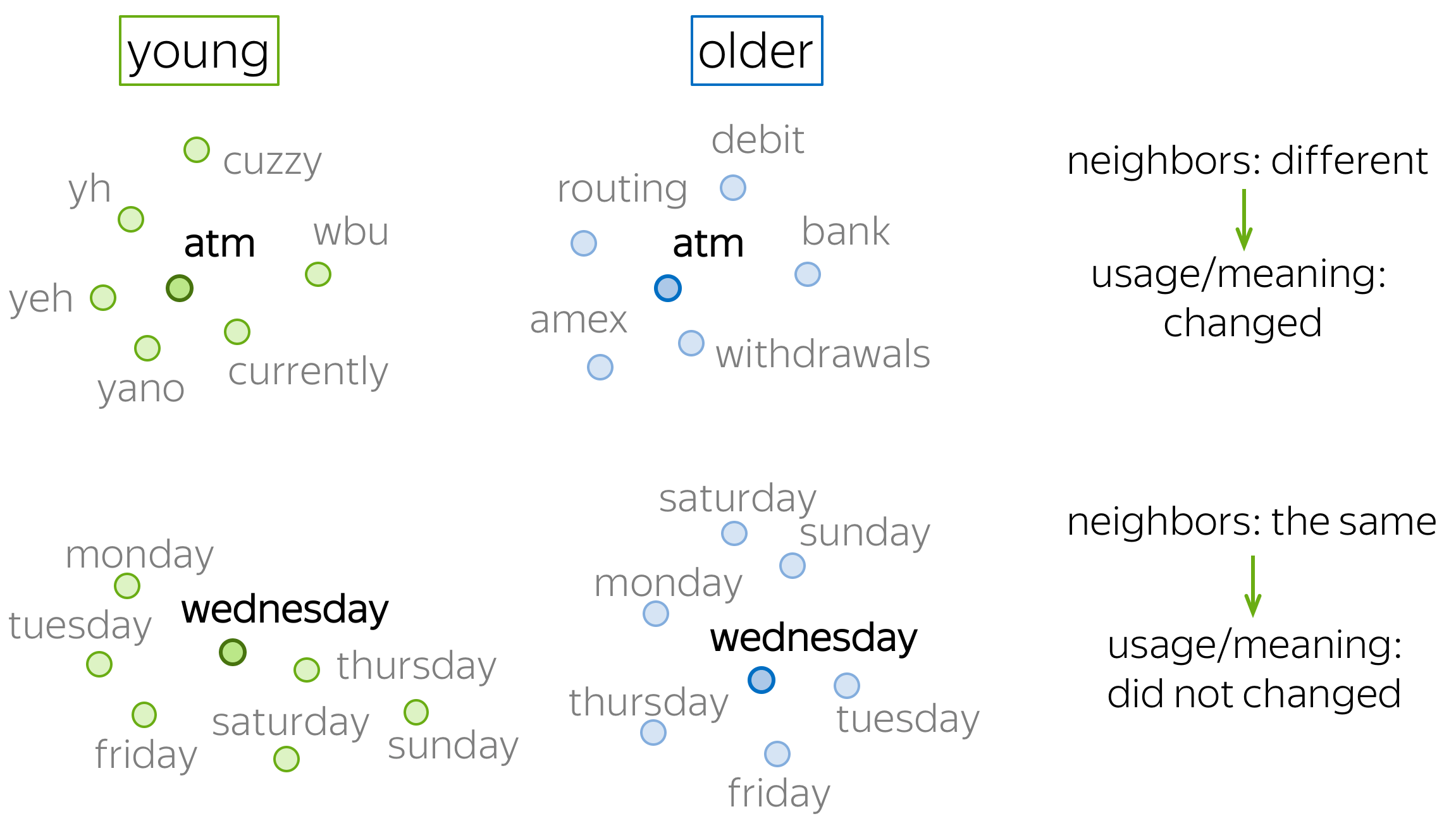
A very simple approach
is to train embeddings (e.g., Word2Vec) and look at the closest neighbors.
If a word’s closest neighbors are different for the two corpora, the word changed
its meaning: remember that word embeddings reflect contexts they saw!
This approach was proposed in
this ACL 2020 paper. Formally, for each word the authors take k nearest neighbors
in the two embeddings sets and count how many neighbors are the same. Large intersection
means that the meaning is not different, small intersection — meaning is different.
Lena: Note that while the approach is recent,
it is extremely simple and works better than previous more complicated ideas.
Never be afraid to try simple things — you’ll be surprised how often they work!
Previous popular approach: align two embedding sets
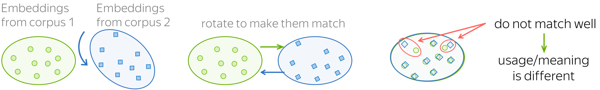
The previous popular approach
was to align two embeddings sets and to find word
whose embeddings do not match well. Formally, let (color{#88a635}{W_1}color{black}, color{#547dbf}{W_2}color{black} in
mathbb{R}^{dtimes |V|})
be embedding sets trained on different corpora.
To align the learned embeddings, the authors find the rotation
(R = arg maxlimits_{Q^TQ=I}parallel color{#547dbf}{W_2}color{black}Q — color{#88a635}{W_1}color{black}parallel_F) — this
is called Orthogonal Procrustes. Using this rotation, we can align embedding sets
and find words which do not match well: these are the words that change
meaning with the corpora.
Lena: You will implement Ortogonal
Proctustes in your homework to align Russian and Ukranian embeddings. Find the notebook in
the course repo.
![]()
Have Fun!
Semantic Space Surfer
Usually, we want word embeddings to reason as humans do. But let’s try the opposite:
you will try to think as word embeddings.
You will see the analogical example, e.g. king — man + woman = ?,
and several possible answers. The task is to guess what word embeddings think.
Complete the task
(10 examples) and get a Semantic Space Surfer Certificate!
Word embeddings: we used glove-twitter-100
from gensim-data.
Big thanks
Just Heuristic for the help with technical issues! Just Heuristic — Just Fun!