What is word clustering

What are Word Clusters?

Word clusters are groups of words based on a common theme. The easiest way to build a cluster is by collecting synonyms for a particular word. The group of synonyms becomes a cluster which has one common meaning and for that one meaning, you have effectively learnt multiple words.

What is the benefit of such an approach?

The benefit of such an approach is: you get to learn group of words with the help of a single meaning. In the language of sets, for one meaning entered into the storage area of your brain, you learn multiple words. This can be labeled as effective usage of memory and that is what we require, don’t we? Also, the multiplicity of learning carries the bigger benefit of rapidly escalating your learning speed. You can learn a vast number of words in a very quick time.

Let’s practice the skill of making clusters:

In this series of articles, we explore two clusters in every article. The two clusters will combine to teach you 10 to 12 words. The theme of the cluster is based on the common meaning for the words. The individual meanings of the distinct words in the cluster are also provided (with every cluster).

Cluster 1: Words related to the sentiment of something being boring or uninteresting

In this group we deal with words that are related to sentiment of something being boring or uninteresting. These words can be used in a variety of situations.

You can go through the words here:

• Banal: Repeated too often.
• Hackneyed: Overfamiliar through overuse.
• Clichéd: Repeated regularly without thought or originality.
• Mundane: Found in the ordinary course of events.
• Humdrum: Not challenging; dull and lacking excitement.
• Vapid: Lacking significance or liveliness or spirit or zest.
• Tedious: So lacking in interest as to cause mental weariness.

Cluster 2: Words related to the sentiment of hatred

In this cluster, explore words related to the sentiment of hatred. These words describe a variety of words related to the sentiment of hating someone. You can identify the ones that you can use in some context as well.

Go through the words here:

• Abhorrence: Hate coupled with disgust.
• Loathing: Find repugnant.
• Disgust: Strong feelings of dislike.
• Odium: State of disgrace resulting from detestable behavior.
• Aversion: A feeling of intense dislike.
• Antipathy: The object of a feeling of intense aversion; something to be avoided.
• The two clusters above showcase how the method of cluster formation can be used for expanding your word-power. Use this method and your vocabulary database will surely grow exponentially.

Best Wishes!!

Кластеризация и визуализация текстовой информации

В русскоязычном секторе интернета очень мало учебных практических примеров (а с примером кода ещё меньше) анализа текстовых сообщений на русском языке. Поэтому я решил собрать данные воедино и рассмотреть пример кластеризации, так как не требуется подготовка данных для обучения.

Большинство используемых библиотек уже есть в дистрибутиве Anaconda 3, поэтому советую использовать его. Недостающие модули/библиотеки можно установить стандартно через pip install «название пакета».
Подключаем следующие библиотеки:

import numpy as np
import pandas as pd
import nltk
import re
import os
import codecs
from sklearn import feature_extraction
import mpld3
import matplotlib.pyplot as plt
import matplotlib as mpl

Для анализа можно взять любые данные. Мне на глаза тогда попала данная задача: Статистика поисковых запросов проекта Госзатраты. Им нужно было разбить данные на три группы: частные, государственные и коммерческие организации. Придумывать экстраординарное ничего не хотелось, поэтому решил проверить, как поведет кластеризация в данном случае (забегая наперед — не очень). Но можно выкачать данные из VK какого-нибудь паблика:

import vk
#передаешь id сессии
session = vk.Session(access_token='')
# URL для получения access_token, вместо tvoi_id вставляете id созданного приложения Вк:
# https://oauth.vk.com/authorize?client_id=tvoi_id&scope=friends,pages,groups,offline&redirect_uri=https://oauth.vk.com/blank.html&display=page&v=5.21&response_type=token 
api = vk.API(session)
poss=[]
id_pab=-59229916 #id пабликов начинаются с минуса, id стены пользователя без минуса
info=api.wall.get(owner_id=id_pab, offset=0, count=1)
kolvo = (info[0]//100)+1

shag=100
sdvig=0
h=0

import time

while h<kolvo:
    if(h>70):
        print(h) #не обязательное условие, просто для контроля примерного окончания процесса
    pubpost=api.wall.get(owner_id=id_pab, offset=sdvig, count=100)
    i=1
    while i < len(pubpost):
        b=pubpost[i]['text']
        poss.append(b)
        i=i+1
    h=h+1
    sdvig=sdvig+shag
    time.sleep(1)
len(poss)

import io
with io.open("public.txt", 'w', encoding='utf-8', errors='ignore') as file:
    for line in poss:
        file.write("%sn" % line)
file.close()

titles = open('public.txt', encoding='utf-8', errors='ignore').read().split('n')

print(str(len(titles)) + ' постов считано')

import re
posti=[]

#удалим все знаки препинания и цифры
for line in titles:
    chis = re.sub(r'(<(/?[^>]+)>)', ' ', line)
    #chis = re.sub()
    chis = re.sub('[^а-яА-Я ]', '', chis)
    posti.append(chis)

Я буду использовать данные поисковых запросов чтобы показать, как плохо кластеризуются короткие текстовые данные. Я заранее очистил от спецсимволов и знаков препинания текст плюс провел замену сокращений (например, ИП – индивидуальный предприниматель). Получился текст, где в каждой строке находился один поисковый запрос.

Считываем данные в массив и приступаем к нормализации – приведению слова к начальной форме. Это можно сделать несколькими способами, используя стеммер Портера, стеммер MyStem и PyMorphy2. Хочу предупредить – MyStem работает через wrapper, поэтому скорость выполнения операций очень медленная. Остановимся на стеммере Портера, хотя никто не мешает использовать другие и комбинировать их с друг другом (например, пройтись PyMorphy2, а после стеммером Портера).

titles = open('material4.csv', 'r', encoding='utf-8', errors='ignore').read().split('n')
print(str(len(titles)) + ' запросов считано')

from nltk.stem.snowball import SnowballStemmer
stemmer = SnowballStemmer("russian")

def token_and_stem(text):
    tokens = [word for sent in nltk.sent_tokenize(text) for word in nltk.word_tokenize(sent)]
    filtered_tokens = []
    for token in tokens:
        if re.search('[а-яА-Я]', token):
            filtered_tokens.append(token)
    stems = [stemmer.stem(t) for t in filtered_tokens]
    return stems

def token_only(text):
    tokens = [word.lower() for sent in nltk.sent_tokenize(text) for word in nltk.word_tokenize(sent)]
    filtered_tokens = []
    for token in tokens:
        if re.search('[а-яА-Я]', token):
            filtered_tokens.append(token)
    return filtered_tokens

#Создаем словари (массивы) из полученных основ
totalvocab_stem = []
totalvocab_token = []
for i in titles:
    allwords_stemmed = token_and_stem(i)
    #print(allwords_stemmed)
    totalvocab_stem.extend(allwords_stemmed)
    
    allwords_tokenized = token_only(i)
    totalvocab_token.extend(allwords_tokenized)

import pymorphy2
morph = pymorphy2.MorphAnalyzer()

G=[]

for i in titles:
    h=i.split(' ')
    #print(h)
    s=''
    for k in h:
        #print(k)
        p = morph.parse(k)[0].normal_form
        #print(p)
        s+=' '
        s += p
        #print(s)
        #G.append(p)
    #print(s)
    G.append(s)

pymof = open('pymof_pod.txt', 'w', encoding='utf-8', errors='ignore')
pymofcsv = open('pymofcsv_pod.csv', 'w', encoding='utf-8', errors='ignore')
for item in G:
    pymof.write("%sn" % item)
    pymofcsv.write("%sn" % item)
pymof.close()
pymofcsv.close()

from pymystem3 import Mystem
m = Mystem()
A = []

for i in titles:
    #print(i)
    lemmas = m.lemmatize(i)
    A.append(lemmas)

#Этот массив можно сохранить в файл либо "забэкапить"
import pickle
with open("mystem.pkl", 'wb') as handle:
                    pickle.dump(A, handle)

Создадим матрицу весов TF-IDF. Будем считать каждый поисковой запрос за документ (так делают при анализе постов в Twitter, где каждый твит – это документ). tfidf_vectorizer мы возьмем из пакета sklearn, а стоп-слова мы возьмем из корпуса ntlk (изначально придется скачать через nltk.download()). Параметры можно подстроить как вы считаете нужным – от верхней и нижней границы до количества n-gram (в данном случае возьмем 3).

stopwords = nltk.corpus.stopwords.words('russian')
#можно расширить список стоп-слов
stopwords.extend(['что', 'это', 'так', 'вот', 'быть', 'как', 'в', 'к', 'на'])

from sklearn.feature_extraction.text import TfidfVectorizer, CountVectorizer

n_featur=200000
tfidf_vectorizer = TfidfVectorizer(max_df=0.8, max_features=10000,
                                 min_df=0.01, stop_words=stopwords,
                                 use_idf=True, tokenizer=token_and_stem, ngram_range=(1,3))
get_ipython().magic('time tfidf_matrix = tfidf_vectorizer.fit_transform(titles)')
print(tfidf_matrix.shape)

Над полученной матрицей начинаем применять различные методы кластеризации:

num_clusters = 5

# Метод к-средних - KMeans
from sklearn.cluster import KMeans

km = KMeans(n_clusters=num_clusters)
get_ipython().magic('time km.fit(tfidf_matrix)')
idx = km.fit(tfidf_matrix)
clusters = km.labels_.tolist()

print(clusters)
print (km.labels_)

# MiniBatchKMeans
from sklearn.cluster import MiniBatchKMeans

mbk  = MiniBatchKMeans(init='random', n_clusters=num_clusters) #(init='k-means++', ‘random’ or an ndarray)
mbk.fit_transform(tfidf_matrix)
%time mbk.fit(tfidf_matrix)
miniclusters = mbk.labels_.tolist()
print (mbk.labels_)


# DBSCAN
from sklearn.cluster import DBSCAN
get_ipython().magic('time db = DBSCAN(eps=0.3, min_samples=10).fit(tfidf_matrix)')
labels = db.labels_
labels.shape
print(labels)

# Аггломеративная класстеризация
from sklearn.cluster import AgglomerativeClustering

agglo1 = AgglomerativeClustering(n_clusters=num_clusters, affinity='euclidean') #affinity можно выбрать любое или попробовать все по очереди: cosine, l1, l2, manhattan
get_ipython().magic('time answer = agglo1.fit_predict(tfidf_matrix.toarray())')
answer.shape

Полученные данные можно сгруппировать в dataframe и посчитать количество запросов, попавших в каждый кластер.

#k-means
clusterkm = km.labels_.tolist()
#minikmeans
clustermbk = mbk.labels_.tolist()
#dbscan
clusters3 = labels
 #agglo
#clusters4 = answer.tolist()

frame = pd.DataFrame(titles, index = [clusterkm])

#k-means
out = { 'title': titles, 'cluster': clusterkm }
frame1 = pd.DataFrame(out, index = [clusterkm], columns = ['title', 'cluster'])

#mini
out = { 'title': titles, 'cluster': clustermbk }
frame_minik = pd.DataFrame(out, index = [clustermbk], columns = ['title', 'cluster'])

frame1['cluster'].value_counts()
frame_minik['cluster'].value_counts()

Из-за большого количества запросов не совсем удобно смотреть таблицы и хотелось бы больше интерактивности для понимания. Поэтому сделаем графики взаимного расположения запросов относительного друг друга.

Сначала необходимо вычислить расстояние между векторами. Для этого будет применяться косинусовое расстояние. В статьях предлагают использовать вычитание из единицы, чтобы не было отрицательных значений и находилось в пределах от 0 до 1, поэтому сделаем так же:

from sklearn.metrics.pairwise import cosine_similarity
dist = 1 - cosine_similarity(tfidf_matrix)
dist.shape

Так как графики будут двух-, трехмерные, а исходная матрица расстояний n-мерная, то придется применять алгоритмы снижения размерности. На выбор есть много алгоритмов (MDS, PCA, t-SNE), но остановим выбор на Incremental PCA. Этот выбор сделан в следствии практического применения – я пробовал MDS и PCA, но оперативной памяти мне не хватало (8 гигабайт) и когда начинал использоваться файл подкачки, то можно было сразу уводить компьютер на перезагрузку.

Алгоритм Incremental PCA используется в качестве замены метода главных компонентов (PCA), когда набор данных, подлежащий разложению, слишком велик, чтобы разместиться в оперативной памяти. IPCA создает низкоуровневое приближение для входных данных, используя объем памяти, который не зависит от количества входных выборок данных.

# Метод главных компонент - PCA

from sklearn.decomposition import IncrementalPCA
icpa = IncrementalPCA(n_components=2, batch_size=16)
get_ipython().magic('time icpa.fit(dist) #demo =')
get_ipython().magic('time demo2 = icpa.transform(dist)')
xs, ys = demo2[:, 0], demo2[:, 1]

# PCA 3D
from sklearn.decomposition import IncrementalPCA
icpa = IncrementalPCA(n_components=3, batch_size=16)
get_ipython().magic('time icpa.fit(dist) #demo =')
get_ipython().magic('time ddd = icpa.transform(dist)')
xs, ys, zs = ddd[:, 0], ddd[:, 1], ddd[:, 2]

#Можно сразу примерно посмотреть, что получится в итоге
#from mpl_toolkits.mplot3d import Axes3D
#fig = plt.figure()
#ax = fig.add_subplot(111, projection='3d')
#ax.scatter(xs, ys, zs)
#ax.set_xlabel('X')
#ax.set_ylabel('Y')
#ax.set_zlabel('Z')
#plt.show()

Перейдем непосредственно к самой визуализации:

from matplotlib import rc
#включаем русские символы на графике
font = {'family' : 'Verdana'}#, 'weigth': 'normal'}
rc('font', **font)

#можно сгенерировать цвета для кластеров
import random
def generate_colors(n):
    color_list = []
    for c in range(0,n):
        r = lambda: random.randint(0,255)
        color_list.append( '#%02X%02X%02X' % (r(),r(),r()) )
    return color_list

#устанавливаем цвета
cluster_colors = {0: '#ff0000', 1: '#ff0066', 2: '#ff0099',  3: '#ff00cc', 4: '#ff00ff',}
#даем имена кластерам, но из-за рандома пусть будут просто 01234
cluster_names = {0: '0',  1: '1', 2: '2',  3: '3', 4: '4',}
#matplotlib inline

#создаем data frame, который содержит координаты (из PCA) + номера кластеров и сами запросы
df = pd.DataFrame(dict(x=xs, y=ys, label=clusterkm, title=titles)) 
#группируем по кластерам
groups = df.groupby('label')

fig, ax = plt.subplots(figsize=(72, 36)) #figsize подбирается под ваш вкус

for name, group in groups:
    ax.plot(group.x, group.y, marker='o', linestyle='', ms=12, label=cluster_names[name], color=cluster_colors[name], mec='none')
    ax.set_aspect('auto')
    ax.tick_params(        axis= 'x',          
        which='both',      
        bottom='off',      
        top='off',         
        labelbottom='off')
    ax.tick_params(        axis= 'y',         
        which='both',     
        left='off',      
        top='off',       
        labelleft='off')
    
ax.legend(numpoints=1)  #показать легенду только 1 точки

#добавляем метки/названия в х,у позиции с поисковым запросом
#for i in range(len(df)):
#    ax.text(df.ix[i]['x'], df.ix[i]['y'], df.ix[i]['title'], size=6)  

#показать график
plt.show() 
plt.close()

Если раскомментировать строку с добавлением названий, то выглядеть это будет примерно так:

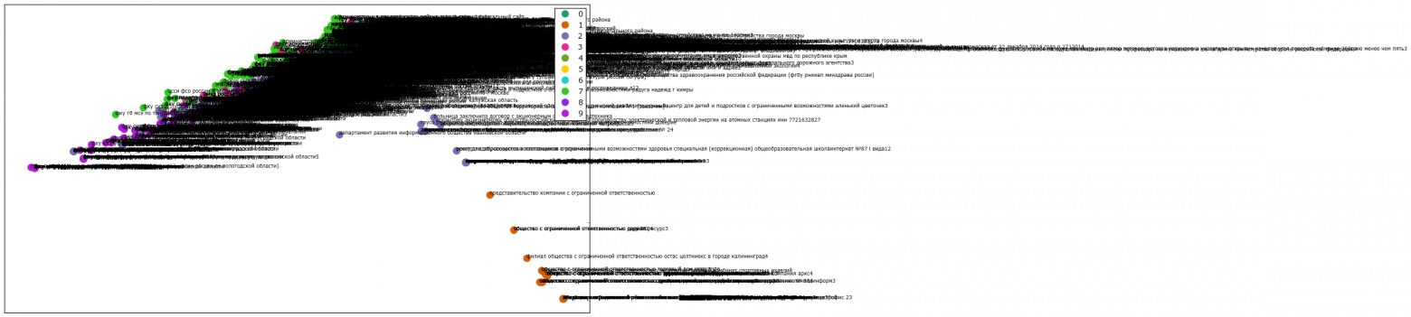
Не совсем то, что хотелось бы ожидать. Воспользуемся mpld3 для перевода рисунка в интерактивный график.

# Plot 
fig, ax = plt.subplots(figsize=(25,27)) 
ax.margins(0.03)


for name, group in groups_mbk:
    points = ax.plot(group.x, group.y, marker='o', linestyle='', ms=12, #ms=18
                     label=cluster_names[name], mec='none', 
                     color=cluster_colors[name])
    ax.set_aspect('auto')
    labels = [i for i in group.title]
    
    tooltip = mpld3.plugins.PointHTMLTooltip(points[0], labels, voffset=10, hoffset=10, #css=css)
    mpld3.plugins.connect(fig, tooltip) #   , TopToolbar()
    
    ax.axes.get_xaxis().set_ticks([])
    ax.axes.get_yaxis().set_ticks([])

    #ax.axes.get_xaxis().set_visible(False)
    #ax.axes.get_yaxis().set_visible(False)

ax.set_title("Mini K-Means", size=20) #groups_mbk
    
ax.legend(numpoints=1)
mpld3.disable_notebook()
#mpld3.display()
mpld3.save_html(fig, "mbk.html")

mpld3.show()
#mpld3.save_json(fig, "vivod.json")
#mpld3.fig_to_html(fig)

fig, ax = plt.subplots(figsize=(51,25))

scatter = ax.scatter(np.random.normal(size=N),
                     np.random.normal(size=N),
                     c=np.random.random(size=N),
                     s=1000 * np.random.random(size=N),
                     alpha=0.3,
                     cmap=plt.cm.jet)
ax.grid(color='white', linestyle='solid')    

ax.set_title("Кластеры", size=20)

fig, ax = plt.subplots(figsize=(51,25))

labels = ['point {0}'.format(i + 1) for i in range(N)]
tooltip = mpld3.plugins.PointLabelTooltip(scatter, labels=labels)
mpld3.plugins.connect(fig, tooltip)

mpld3.show()fig, ax = plt.subplots(figsize=(72,36))
for name, group in groups:
    points = ax.plot(group.x, group.y, marker='o', linestyle='', ms=18, 
                     label=cluster_names[name], mec='none', 
                     color=cluster_colors[name])
    ax.set_aspect('auto')
    labels = [i for i in group.title]
    tooltip = mpld3.plugins.PointLabelTooltip(points, labels=labels)
    mpld3.plugins.connect(fig, tooltip)

ax.set_title("K-means", size=20)

mpld3.display()

Теперь при наведении на любую точку графика всплывает текст с соотвествующим поисковым запросом. Пример готового html файла можно посмотреть здесь: Mini K-Means

Если хочется в 3D и с изменяемым масштабом, то существует сервис Plotly, который имеет плагин для Python.

#для примера просто 3D график из полученных значений
import plotly
plotly.__version__

import plotly.plotly as py
import plotly.graph_objs as go

trace1 = go.Scatter3d(
    x=xs,
    y=ys,
    z=zs,
    mode='markers',
    marker=dict(
        size=12,
        line=dict(
            color='rgba(217, 217, 217, 0.14)',
            width=0.5
        ),
        opacity=0.8
    )
)

data = [trace1]
layout = go.Layout(
    margin=dict(
        l=0,
        r=0,
        b=0,
        t=0
    )
)
fig = go.Figure(data=data, layout=layout)
py.iplot(fig, filename='cluster-3d-plot')

Результаты можно увидеть здесь: Пример

И заключительным пунктом выполним иерархическую (аггломеративную) кластеризацию по методу Уорда для создания дендограммы.

In [44]:
from scipy.cluster.hierarchy import ward, dendrogram
linkage_matrix = ward(dist)

fig, ax = plt.subplots(figsize=(15, 20))
ax = dendrogram(linkage_matrix, orientation="right", labels=titles);

plt.tick_params(
    axis= 'x',
    which='both', 
    bottom='off',
    top='off',
    labelbottom='off')

plt.tight_layout() 

#сохраним рисунок
plt.savefig('ward_clusters2.png', dpi=200)

Выводы

К сожалению, в области исследования естественного языка очень много нерешённых вопросов и не все данные легко и просто сгруппировать в конкретные группы. Но надеюсь, что данное руководство усилит интерес к данной теме и даст базис для дальнейших экспериментов.

Весь код доступен по ссылке: https://github.com/OlegBezverhii/python-notebooks/blob/master/ClasteringRus.py

A cluster is defined as “a small, close group.” Word Clusters are groups of words sharing the same global con- cept. For example, house, cabin, mansion, and shack are similar in that they are all forms of shelter.

What is clustering in reading?

Clustering is a type of pre-writing that allows a writer to explore many ideas as soon as they occur to them. Like brainstorming or free associating, clustering allows a writer to begin without clear ideas. Write quickly, circling each word, and group words around the central word.

What is a clustering strategy?

Cluster Strategy: Promote business clusters by focusing resources and regulatory policies toward developing and retaining businesses in a number of discrete sectors that demonstrate opportunity to advance City goals and enhance the region’s economic strength.

What are the 4 reading strategies?

Figure. Reciprocal teaching is a scaffolded, or supported, discussion technique that incorporates four main strategies—predicting, questioning, clarifying, summarizing—that good readers use together to comprehend text. Think about how you use these strategies in your own reading as an adult.

What is clustering of ideas?

Clustering is used to organize and analyse large numbers of ideas by categorising them. By organising and reorganising ideas, students gain a better appreciation of, and dialogue about, their ideas. As students create idea clusters, new contexts and connections among themes emerge.

What is cluster method in teaching?

Cluster grouping is an educational process in which four to six gifted and talented (GT) or high-achieving students or both are assigned to an otherwise heterogeneous classroom within their grade to be instructed by a teacher who has had specialized training in differentiating for gifted learners.

What is cluster in simple English?

A cluster is a small group of people or things. When you and your friends huddle awkwardly around the snack table at a party, whispering and trying to muster enough nerve to hit the dance floor, you’ve formed a cluster. Cluster comes to us from the Old English word clyster, meaning bunch.

What is cluster concept?

A cluster concept is one that is defined by a weighted list of criteria, such that no one of these criteria is either necessary or sufficient for membership. People say, for instance, that democracy is a cluster concept; Denis Dutton has recently argued that art is a cluster concept. …