
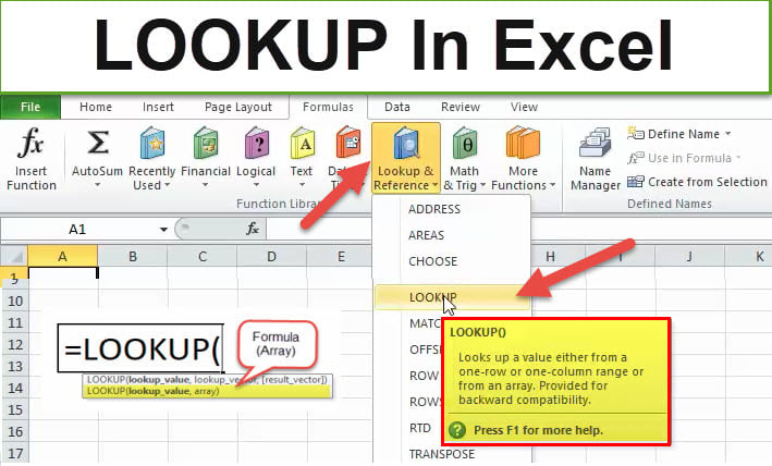
Use LOOKUP, one of the lookup and reference functions, when you need to look in a single row or column and find a value from the same position in a second row or column.
For example, let’s say you know the part number for an auto part, but you don’t know the price. You can use the LOOKUP function to return the price in cell H2 when you enter the auto part number in cell H1.
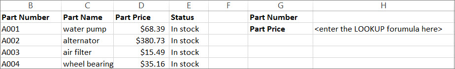
Use the LOOKUP function to search one row or one column. In the above example, we’re searching prices in column D.
Tips: Consider one of the newer lookup functions, depending on which version you are using.
-
Use VLOOKUP to search one row or column, or to search multiple rows and columns (like a table). It’s a much improved version of LOOKUP. Watch this video about how to use VLOOKUP.
-
If you are using Microsoft 365, use XLOOKUP — it’s not only faster, it also lets you search in any direction (up, down, left, right).
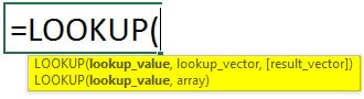
There are two ways to use LOOKUP: Vector form and Array form
-
Vector form: Use this form of LOOKUP to search one row or one column for a value. Use the vector form when you want to specify the range that contains the values that you want to match. For example, if you want to search for a value in column A, down to row 6.

-
Array form: We strongly recommend using VLOOKUP or HLOOKUP instead of the array form. Watch this video about using VLOOKUP. The array form is provided for compatibility with other spreadsheet programs, but it’s functionality is limited.
An array is a collection of values in rows and columns (like a table) that you want to search. For example, if you want to search columns A and B, down to row 6. LOOKUP will return the nearest match. To use the array form, your data must be sorted.
Vector form
The vector form of LOOKUP looks in a one-row or one-column range (known as a vector) for a value and returns a value from the same position in a second one-row or one-column range.
Syntax
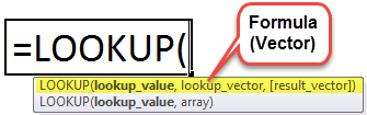
LOOKUP(lookup_value, lookup_vector, [result_vector])
The LOOKUP function vector form syntax has the following arguments:
-
lookup_value Required. A value that LOOKUP searches for in the first vector. Lookup_value can be a number, text, a logical value, or a name or reference that refers to a value.
-
lookup_vector Required. A range that contains only one row or one column. The values in lookup_vector can be text, numbers, or logical values.
Important: The values in lookup_vector must be placed in ascending order: …, -2, -1, 0, 1, 2, …, A-Z, FALSE, TRUE; otherwise, LOOKUP might not return the correct value. Uppercase and lowercase text are equivalent.
-
result_vector Optional. A range that contains only one row or column. The result_vector argument must be the same size as lookup_vector. It has to be the same size.
Remarks
-
If the LOOKUP function can’t find the lookup_value, the function matches the largest value in lookup_vector that is less than or equal to lookup_value.
-
If lookup_value is smaller than the smallest value in lookup_vector, LOOKUP returns the #N/A error value.
Vector examples
You can try out these examples in your own Excel worksheet to learn how the LOOKUP function works. In the first example, you’re going to end up with a spreadsheet that looks similar to this one:
-
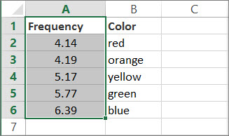
Copy the data in following table, and paste it into a new Excel worksheet.
Copy this data into column A
Copy this data into column B
Frequency
4.14
Color
red
4.19
orange
5.17
yellow
5.77
green
6.39
blue
-
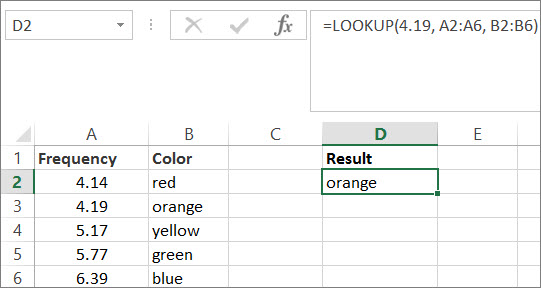
Next, copy the LOOKUP formulas from the following table into column D of your worksheet.
Copy this formula into the D column
Here’s what this formula does
Here’s the result you’ll see
Formula
=LOOKUP(4.19, A2:A6, B2:B6)
Looks up 4.19 in column A, and returns the value from column B that is in the same row.
orange
=LOOKUP(5.75, A2:A6, B2:B6)
Looks up 5.75 in column A, matches the nearest smaller value (5.17), and returns the value from column B that is in the same row.
yellow
=LOOKUP(7.66, A2:A6, B2:B6)
Looks up 7.66 in column A, matches the nearest smaller value (6.39), and returns the value from column B that is in the same row.
blue
=LOOKUP(0, A2:A6, B2:B6)
Looks up 0 in column A, and returns an error because 0 is less than the smallest value (4.14) in column A.
#N/A
-
For these formulas to show results, you may need to select them in your Excel worksheet, press F2, and then press Enter. If you need to, adjust the column widths to see all the data.
Array form
The array form of LOOKUP looks in the first row or column of an array for the specified value and returns a value from the same position in the last row or column of the array. Use this form of LOOKUP when the values that you want to match are in the first row or column of the array.
Syntax
LOOKUP(lookup_value, array)
The LOOKUP function array form syntax has these arguments:
-
lookup_value Required. A value that LOOKUP searches for in an array. The lookup_value argument can be a number, text, a logical value, or a name or reference that refers to a value.
-
If LOOKUP can’t find the value of lookup_value, it uses the largest value in the array that is less than or equal to lookup_value.
-
If the value of lookup_value is smaller than the smallest value in the first row or column (depending on the array dimensions), LOOKUP returns the #N/A error value.
-
-
array Required. A range of cells that contains text, numbers, or logical values that you want to compare with lookup_value.
The array form of LOOKUP is very similar to the HLOOKUP and VLOOKUP functions. The difference is that HLOOKUP searches for the value of lookup_value in the first row, VLOOKUP searches in the first column, and LOOKUP searches according to the dimensions of array.
-
If array covers an area that is wider than it is tall (more columns than rows), LOOKUP searches for the value of lookup_value in the first row.
-
If an array is square or is taller than it is wide (more rows than columns), LOOKUP searches in the first column.
-
With the HLOOKUP and VLOOKUP functions, you can index down or across, but LOOKUP always selects the last value in the row or column.
Important: The values in array must be placed in ascending order: …, -2, -1, 0, 1, 2, …, A-Z, FALSE, TRUE; otherwise, LOOKUP might not return the correct value. Uppercase and lowercase text are equivalent.
-
This Excel tutorial explains how to use the Excel LOOKUP function with syntax and examples.
Description
The Microsoft Excel LOOKUP function returns a value from a range (one row or one column) or from an array.
The LOOKUP function is a built-in function in Excel that is categorized as a Lookup/Reference Function. It can be used as a worksheet function (WS) in Excel. As a worksheet function, the LOOKUP function can be entered as part of a formula in a cell of a worksheet.
There are 2 different syntaxes for the LOOKUP function:
LOOKUP Function (Syntax #1)
In Syntax #1, the LOOKUP function searches for value in the lookup_range and returns the value in the result_range that is in the same position.
The syntax for the LOOKUP function in Microsoft Excel is:
LOOKUP( value, lookup_range, [result_range] )
Parameters or Arguments
- value
- The value to search for in the lookup_range.
- lookup_range
- A single row or single column of data that is sorted in ascending order. The LOOKUP function searches for value in this range.
- result_range
- Optional. It is a single row or single column of data that is the same size as the lookup_range. The LOOKUP function searches for the value in the lookup_range and returns the value from the same position in the result_range. If this parameter is omitted, it will return the first column of data.
Returns
The LOOKUP function returns any datatype such as a string, numeric, date, etc.
If the LOOKUP function can not find an exact match, it chooses the largest value in the lookup_range that is less than or equal to the value.
If the value is smaller than all of the values in the lookup_range, then the LOOKUP function will return #N/A.
If the values in the LOOKUP_range are not sorted in ascending order, the LOOKUP function will return the incorrect value.
Example (as Worksheet Function)
Let’s look at some Excel LOOKUP function examples and explore how to use the LOOKUP function as a worksheet function in Microsoft Excel:
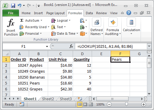
Based on the Excel spreadsheet above, the following LOOKUP examples would return:
=LOOKUP(10251, A1:A6, B1:B6)
Result: "Pears"

=LOOKUP(10251, A1:A6)
Result: 10251

=LOOKUP(10246, A1:A6, B1:B6)
Result: #N/A

=LOOKUP(10248, A1:A6, B1:B6)
Result: "Apples"
LOOKUP Function (Syntax #2)
In Syntax #2, the LOOKUP function searches for the value in the first row or column of the array and returns the corresponding value in the last row or column of the array.
The syntax for the LOOKUP function in Microsoft Excel is:
LOOKUP( value, array )
Parameters or Arguments
- value
- The value to search for in the array. The values must be in ascending order.
- array
- An array of values that contains both the values to search for and return.
Returns
The LOOKUP function returns any datatype such as a string, numeric, date, etc.
If the LOOKUP function can not find an exact match, it chooses the largest value in the lookup_range that is less than or equal to the value.
If the value is smaller than all of the values in the lookup_range, then the LOOKUP function will return #N/A.
If the values in the array are not sorted in ascending order, the LOOKUP function will return the incorrect value.
Example (as Worksheet Function)
Let’s look at some Excel LOOKUP function examples and explore how to use the LOOKUP function as a worksheet function in Microsoft Excel:
=LOOKUP("T", {"s","t","u","v";10,11,12,13})
Result: 11

=LOOKUP("Tech on the Net", {"s","t","u","v";10,11,12,13})
Result: 11

=LOOKUP("t", {"s","t","u","v";"a","b","c","d"})
Result: "b"

=LOOKUP("r", {"s","t","u","v";"a","b","c","d"})
Result: #N/A

=LOOKUP(2, {1,2,3,4;511,512,513,514})
Result: 512
Frequently Asked Questions
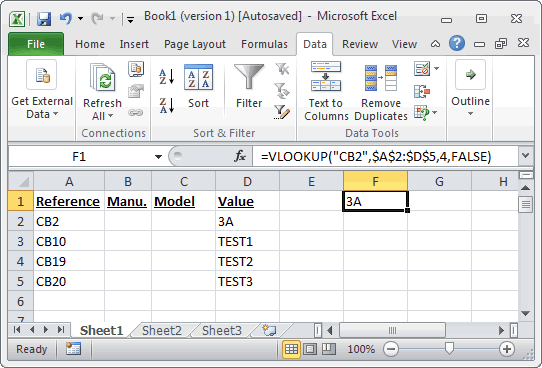
Question: In Microsoft Excel, I have a table of data in cells A2:D5. I’ve tried to create a simple LOOKUP to find CB2 in the data, but it always returns 0. What am I doing wrong?
Answer: Using the LOOKUP function can sometimes be a bit tricky so let’s look at an example. Below we have a spreadsheet with the data that you described.
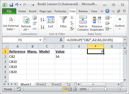
In cell F1, we’ve placed the following formula:
=LOOKUP("CB2",A2:A5,D2:D5)
And yes, even though CB2 exists in the data, the LOOKUP function returns 0.
Now, let’s explain what is happening. At first, it looks like the function isn’t finding CB2 in the list, but in fact, it is finding something else. Let’s fill in the empty cells in D3:D5 to explain better.
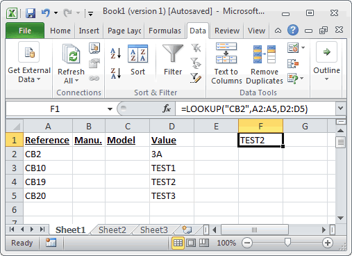
If we place the values TEST1, TEST2, TEST3 in cells D3, D4, 5, respectively, we can see that the LOOKUP function is in fact returning the value TEST2. So we ask ourselves, when we are looking up CB2 in the data and CB2 exists in the data, why is it returning the value for CB19? Good question. The LOOKUP function assumes that the data in column A is sorted in ascending order.
If you look closer at column A, it is not in fact sorted in ascending order. If we quickly sorted column A, it would look like this:
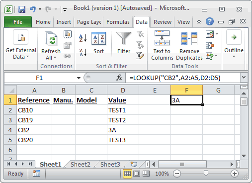
Now the LOOKUP function correctly returns 3A when it is looking up CB2 in the data.
To avoid these sorting problems with your data, we recommend using VLOOKUP function in this case. Let’s show you how we would do this. If we changed our formula below (but left our data in column A in the original sort order):
The following VLOOKUP formula would return the correct value of 3A.
=VLOOKUP("CB2",$A$2:$D$5,4,FALSE)
The VLOOKUP function does not require us to have the data sorted in ascending order since we used FALSE as the last parameter — which means that it is looking for an exact match.
Question: I have the following LOOKUP formula:
=LOOKUP(C2,{"A","B","C","D","E","F","G","H","I","K","X","Z"}, {"1","2","3","4","5","6","7","8","9","10","12","1"})
I also need to add zero to the lookup vector and result vector. How do I do this?
Answer: Using numbers in Excel can be tricky, as you can enter them either as numeric or text values. Because of this, there are 2 possible solutions.
Numeric Solution
If you have entered your zero as a numeric value, then the following formula will work:
=LOOKUP(C2,{0,"A","B","C","D","E","F","G","H","I","K","X","Z"}, {0,"1","2","3","4","5","6","7","8","9","10","12","1"})
Text Solution
If you have entered your zero as a text value, then the following formula will work:
=LOOKUP(C2,{"0","A","B","C","D","E","F","G","H","I","K","X","Z"}, {"0","1","2","3","4","5","6","7","8","9","10","12","1"})
Question: For the following function in Microsoft Excel:
=LOOKUP(M14,Sheet2!A2:A2240,Sheet2!B2:B2240)
How do I get it to return a blank cell if the LOOKUP value (M14) is blank?
Answer: To check for a blank value in cell M14, you can use the IF function and ISBLANK function as follows:
=IF(ISBLANK(M14),"",LOOKUP(M14,Sheet2!A2:A2240,Sheet2!B2:B2240))
Now if the value in cell M14 is blank, the formula will return a blank. Otherwise it will perform the LOOKUP function as before.
The LOOKUP excel function searches a value in a range (single row or single column) and returns a corresponding match from the same position of another range (single row or single column). The corresponding match is a piece of information associated with the value being searched.
For example, the branch code (search value) can be used to retrieve the profits of different bank branches (corresponding match). Being a lookup and reference function, the LOOKUP has two varieties–vector and array.
The VLOOKUPThe VLOOKUP excel function searches for a particular value and returns a corresponding match based on a unique identifier. A unique identifier is uniquely associated with all the records of the database. For instance, employee ID, student roll number, customer contact number, seller email address, etc., are unique identifiers.
read more and HLOOKUPHlookup is a referencing worksheet function that finds and matches the value from a row rather than a column using a reference. Hlookup stands for horizontal lookup, in which we search for data in rows horizontally.read more are improved versions of the LOOKUP function.
The LOOKUP is different from the VLOOKUP function in the sense that the former looks for a match in a one-row or one-column range while the latter searches the entire data table.
Table of contents
- What is LOOKUP Excel Function?
- LOOKUP Excel Function–Syntax 1 (Vector Form)
- LOOKUP Excel Function–Syntax 2 (Array Form)
- The Explanation of the LOOKUP Function
- How to use the LOOKUP Function in Excel?
- Example #1–Vector Form
- Example #2–Vector Form
- Example #3–Vector Form
- Example #4–Array Form
- Applications
- Frequently Asked Questions
- LOOKUP Excel Video
- Recommended Articles
LOOKUP Excel Function–Syntax 1 (Vector Form)
In the present context, a one-row or one-column range is known as a vector. In this form, the function searches a particular value in one vector and returns a corresponding value at the same position from another vector.
The syntax of the vector form is shown in the following image:
The function accepts the following arguments in the vector form:
- Lookup_value: This is the value to be searched.
- Lookup_vector: This is the one-row or one-column range in which the value is to be searched. It should be sorted in alphabetical order or ascending order to obtain correct results.
- Result_vector: This is the one-row or one-column range from which the output is to be returned. The output returned is in the same position as the “lookup_value.”
The “lookup_value” and “lookup_vector” are mandatory arguments while “result_vector” is optional.
Note: The “lookup_vector” and the “result_vector” both are one-row or one-column range with the same size. If the latter is omitted, Excel returns a value from the former.
LOOKUP Excel Function–Syntax 2 (Array Form)
In this form, the function searches a specified value in the first row or column of the array and returns a corresponding value at the same position from the last row or column of the array.
The syntax of the array form is shown in the following image:

The function accepts the following mandatory arguments in the array form:
- Lookup_value: This is the value to be searched.
- Array: This is the array or range where the value is to be searched.
The first row or column of the array is similar to the “lookup_vector” (vector form). The last row or column of the array is similar to the “result_vector” (vector form).
The Explanation of the LOOKUP Function
The LOOKUP function works on a close match or an approximate match. The two forms of the function are explained in the current section.
The Vector Form
The LOOKUP function looks for the exact “lookup_value” in the “lookup_vector” and returns the output at the same position from the “result_vector.” The possibilities are stated as follows:
- If the function does not find an exact match, it looks up the largest value in the “lookup_vector,” which is less than or equal to the “lookup_value.”
- If the “lookup_value” is smaller than all the values of the “lookup_vector,” the function returns “#N/A error”.
- If the “lookup_value” is greater than all the values of the “lookup_vector,” the function matches with the last value of the array.
- If the “lookup_value” occurs multiple times in the “lookup_vector,” the function considers the last occurrence of the former.
The “lookup_value,” “lookup_vector,” and “result_vector” can be a number, text string, date, currency, and so on.
The Array Form
The LOOKUP function searches for a value according to the dimensions (size) of the array. The possibilities are stated as follows:
- If the number of rows is more than the columns (column size is greater than or equal to the row size), the function searches for the “lookup_value” in the first column.
- If the number of columns is more than the rows (row size is greater than the column size), the function searches for the “lookup_value” in the first row.
You are free to use this image on your website, templates, etc, Please provide us with an attribution linkArticle Link to be Hyperlinked
For eg:
Source: LOOKUP Excel Function (wallstreetmojo.com)
How to use the LOOKUP Function in Excel?
Let us understand the working of the LOOKUP function with the help of examples.
You can download this LOOKUP Function Excel Template here – LOOKUP Function Excel Template
Example #1–Vector Form
The succeeding table shows a list of flowers, the identifier (ID), and the current price. The output to be retrieved with the help of the LOOKUP function is stated as follows:
a. The price of the flower given its ID
b. The price of the flower given its name
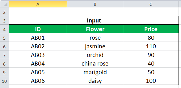
a. We use the following syntax for extracting the price of the flower with its ID.
“=LOOKUP(ID_to_search,A5:A10,C5:C10)”
Since the value to be searched can be supplied as a cell reference, enter E5 in the formula. This is shown in the succeeding image.
“=LOOKUP(E5,A5:A10,C5:C10)”
The formula returns 50.

b. We use the following formula for extracting the price of the flower with its name.
“=LOOKUP(“orchid”,B5:B10,C5:C10)”
The formula returns 90.
Example #2–Vector Form
The following table displays the transaction costs (in dollars) incurred on various dates beginning from January 2009. The output to be retrieved with the help of the LOOKUP function is stated as follows:
a. The cost of the last transaction of 2012
b. The cost of the last transaction of March

a. We use the following formula for extracting information on the last transaction of 2012.
“=LOOKUP(D4,YEAR(A4:A18),B4:B18)”
The “YEAR(A4:A18)” retrieves the year from the dates given in A4:A18. Since D4=2012, the formula returns $40000.

b. We use the following formula for extracting the cost of the last transaction of March.
“=LOOKUP(3,MONTH(A4:A18),B4:B18)”
The “MONTH(A4:A18)” extracts the month from the dates given in A4:A18. The formula returns $110000.
Example #3–Vector Form
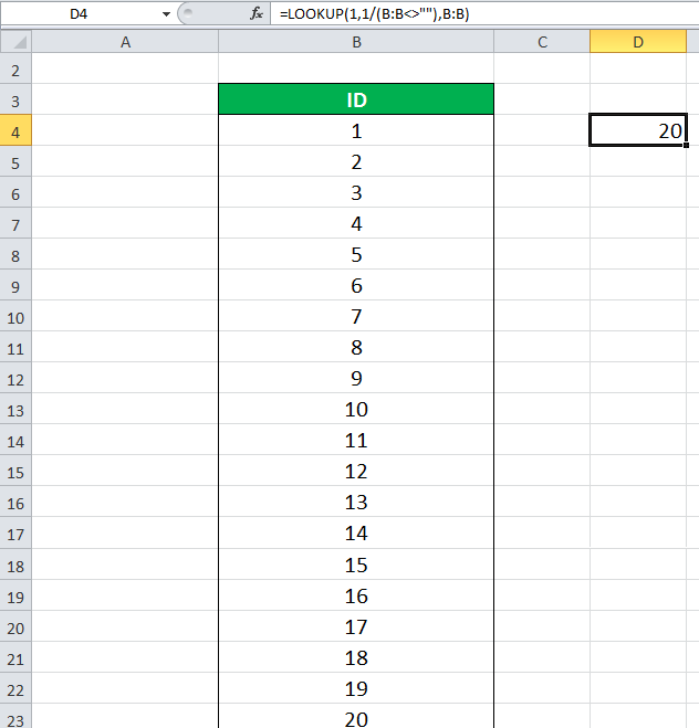
The following table shows a list of IDs in column B. We want to retrieve the last entry of the column with the help of the LOOKUP function. The situations for retrieval are stated as follows:
a. When IDs are listed from 1 to 10
b. When IDs are listed from 1 to 20

a. We use the following formula to extract the last entry of column B.
“=LOOKUP(1,1/(B:B<>””),B:B)”
In the formula, the “lookup_value” is 1, the “lookup_vector” is 1/(B:B<>””), and the “result_vector” is B:B.
The (B:B<>””) forms an array of “true” and “false” where the former means a value is present, while the latter means it is absent. This array is divided by 1 to form another array of “1” and “0” which corresponds to “true” and “false” respectively.
Since the “lookup_value” is 1, the LOOKUP function looks for 1 in the array of “1” and “0.” It matches the “lookup_value” with the last “1” and returns a corresponding match. In this case, the corresponding match is the actual “lookup_value” at the same position, which is 10.
The output of the formula is 10, as shown in the following image.

b. We use the same formula (explained in the preceding section) to extract the last entry of column B.
“=LOOKUP(1,1/(B:B<>””),B:B)”
The formula returns 20, as shown in the following image.
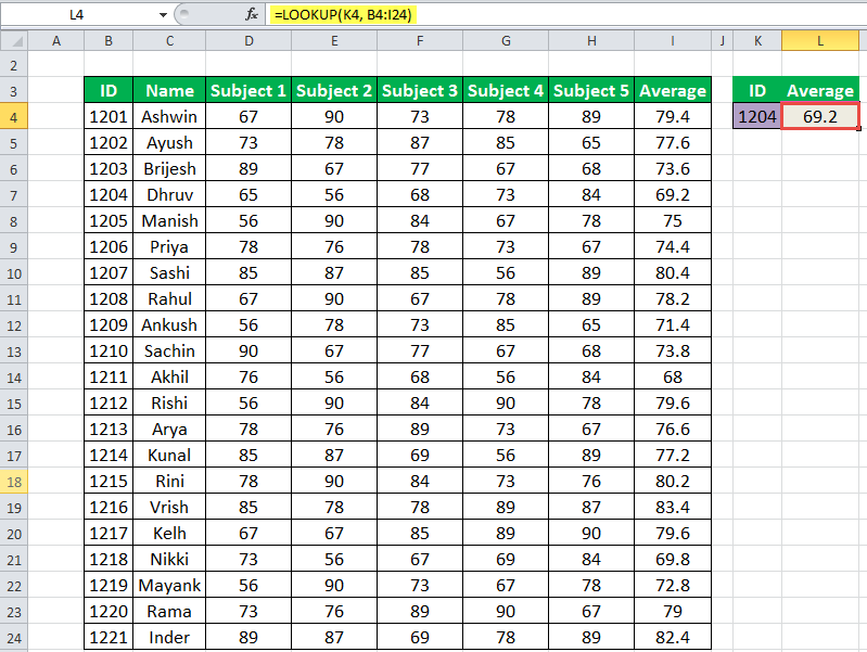
Example #4–Array Form
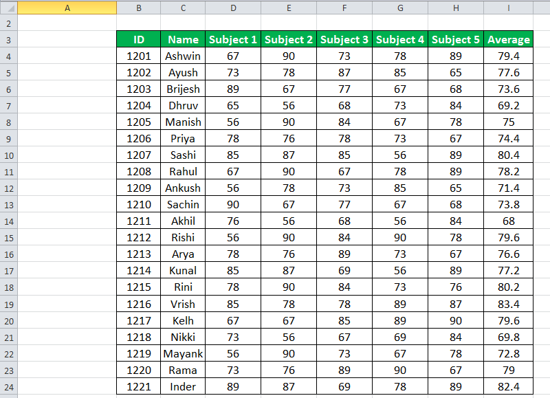
The following table (B3:I24) shows the roll numbers (ID), names of the students, marks in five subjects, and average marks. We want to retrieve the average marks with the help of the student ID.
Since the ID to look for is in cell K4, the following formula is used.
“=LOOKUP(K4,B4:I24)”
The formula returns the corresponding average marks of the student Dhruv (ID 1204). The output is 69.2, as shown in the following image.
Applications
The function is used in the following situations:
- To extract the price of an item using its identifier
- To find the location of a book in the library
- To obtain the last transaction cost for a given month or year
- To check the latest price of a product
- To find the last row within a range of numerical or textual data
- To retrieve the last transaction date
Note: The LOOKUP function of Excel is not case-sensitive implying that it treats the uppercase and lowercase letters the same.
Frequently Asked Questions
Define the LOOKUP function of Excel.
The LOOKUP function looks for a value in a single row or column and returns a corresponding value having the same position from another row or column. The look up and the extraction data both should be a one-row or a one-column range.
The LOOKUP function of Excel has two forms which are explained as follows:
• Vector form–The “lookup_value” is searched in the “lookup_vector” and a corresponding match is returned from the “result_vector.” The syntax is stated as follows:
“LOOKUP(lookup_value,lookup_vector,[result_vector])”
The first two arguments are mandatory and the last one is optional.
• Array form–The “lookup_value” is searched in the first row or column of the “array” and a corresponding match is returned from the last row or column of the “array.” The syntax is stated as follows:
“LOOKUP(lookup_value,array)”
Both the arguments are mandatory.
When should the LOOKUP function of Excel be used?
The usage of the general LOOKUP function, the vector, and the array forms is mentioned as follows:
• The general function is used when there is a need to retrieve an associated piece of information from a one-row or a one-column range.
• The vector form is used when there is a need to specify the range from which a corresponding match is to be returned.
• The array form is used when the lookup or search value is in the first row or column and the corresponding match is in the last row or column.
Note: It is recommended to use the VLOOKUP and HLOOKUP as an alternative to the array form.
What is the difference between the LOOKUP, VLOOKUP, and HLOOKUP functions of Excel?
The differences between the three functions are stated as follows:
• The LOOKUP searches for a value in a one-row or one-column range. In contrast, the VLOOKUP and HLOOKUP search for a value in two or more columns or rows respectively.
• The array form of the LOOKUP searches the “lookup_value” according to the dimensions of the array. In comparison, the VLOOKUP and the HLOOKUP search for the “lookup_value” in the first column and the first row respectively.
• The LOOKUP looks for an approximate match while the VLOOKUP and HLOOKUP work for both approximate and exact matches.
• The LOOKUP has cross functionality implying that it is capable of performing both vertical and horizontal lookups. On the other hand, the VLOOKUP and HLOOKUP are limited to only vertical and horizontal lookups respectively.
LOOKUP Excel Video
Recommended Articles
This has been a tutorial to LOOKUP Excel function. Here we discuss how to use LOOKUP formula along with step by step practical examples. You can download the Excel template from the website. You may also go through these useful functions in Excel-
- Power BI VlookupVLOOKUP in Power BI helps the users fetch data from the other tables. Since it is not an inbuilt function, the user needs to replicate it using the DAX function like the LOOKUPVALUE DAX function.read more
- VBA LOOKUPLOOKUP is the function to fetch the data from the main table based on a single lookup value. VBA LOOKUP function doesn’t require a data structure like that. It doesn’t matter whether the result column is to the right or left. It can fetch the data comfortably.read more
- Excel VLOOKUP FormulaThe VLOOKUP excel function searches for a particular value and returns a corresponding match based on a unique identifier. A unique identifier is uniquely associated with all the records of the database. For instance, employee ID, student roll number, customer contact number, seller email address, etc., are unique identifiers.
read more - Degrees Function in ExcelDEGREES function in excel is used to convert the angles mentioned in radians which are determined based on the radius of a circle to degrees. It is one of the mathematical and trigonometric functions inbuilt into Excel to resolve the problem with radians.read more
- Excel TroubleshootingTroubleshooting in Excel helps when we tend to get some errors or unexpected results associated with the formula we use in Excel. read more
![]()
Download Article
![]()
Download Article
Whenever you keep track of data in spreadsheets, there’ll come a time when you want to find information without having to scroll through endless columns or rows. We’ll show you how to use Microsoft Excel’s LOOKUP function to find a value from one row or column in a different row or column. If you’re looking to do a reverse Vlookup, check out How to Do a Reverse Vlookup in Google Sheets.
Steps
-
1
Create a two column list toward the bottom of the page. In this example, one column has numbers and the other has random words.
-
2
Decide on cell that you would like the user to select from, this is where a drop down list will be.
Advertisement
-
3
Once you click on the cell, the border should darken, select the DATA tab on the tool bar, then select VALIDATION.
-
4
A pop up should appear, in the ALLOW list pick LIST.
-
5
Now to pick your source, in other words your first column, select the button with the red arrow.
-
6
Select the first column of your list and press enter and click OK when the data validation window appears, now you should see a box with an arrow on, if you click on it your list should drop down.
-
7
Select another box where you want the other information to show up.
-
8
Once you clicked that box, go to the INSERT tab and FUNCTION.
-
9
Once the box pops up, select LOOKUP & REFERENCE from the category list.
-
10
Find LOOKUP in the list and double-click it, another box should appear click OK.
-
11
For the lookup_value select the cell with the drop down list.
-
12
For the Lookup_vector select the first column of your list.
-
13
For the Result_vector select the second column.
-
14
Now whenever you pick something from the drop down list the info should automatically change.


Advertisement
Ask a Question
200 characters left
Include your email address to get a message when this question is answered.
Submit
Advertisement
Video
-
Whenever you are completed you can change the font color to white, to make the list hidden.
-
Save your work constantly, especially if the list is extensive
-
Make sure when you are in the DATA VALIDATION window (Step 5) the box labeled IN-CELL DROPDOWN is checked
Show More Tips
Thanks for submitting a tip for review!
Advertisement
About This Article
Thanks to all authors for creating a page that has been read 312,656 times.
Is this article up to date?
LOOKUPS in Excel Explained
Lookup functions are some of the most used Excel functions.
What is a Lookup?
I’m glad you asked. Lookups effectively search for a particular value in a row or column and return a corresponding value from another row or column. A Lookup allows you to search for specific values based on neighboring values.
They can be incredibly useful when you have large datasets or many worksheets that you need to search across.
In this guide to Lookups, we explain the different Lookup functions. We start with LOOKUP, then move onto Vertical Lookup (VLOOKUP), Horizontal Lookup (HLOOKUP), and end with the incredibly powerful XLOOKUP and INDEX-MATCH functions.
First, we’ll look at the syntax for the basic LOOKUP function and how those parameters break down.
Table of Contents
1. LOOKUP
The LOOKUP function searches for a value in the lookup_vector and returns the corresponding value in the result_vector.
Syntax
=LOOKUP (lookup_value, lookup_vector, [result_vector])
If that sounds confusing, don’t worry, we’ll explain everything with a few examples in a moment.
The best way to look at any function is to work through its syntax. By breaking down the function like this, we start to understand how it operates.
Parameters
- lookup_value – Specifies the value to search for in the lookup range (lookup_vector).
- lookup_vector – Specifies a single row or column of data in ascending order that you want the function to search in.
- result_vector – This is optional. The information in the result_vector is returned if the result_vector parameter is used!
Example 1
Here we are looking up the salary of employee Number 23. Our Lookup value is 23, our lookup vector is A2 to A5, and our results vector is D2 to D5.
Example 2
The LOOKUP function comes into its own when you understand how it matches values when it cannot find an exact match.
In this example, the LOOKUP function cannot find an exact match:
=LOOKUP(1010, A3:A6, B3:B6)
Therefore, it chooses the next highest value in the lookup_vector that is less than or equal to the lookup_value.
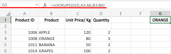
In this instance, as the value 1010 is not available in the lookup_range, Excel chooses the highest value below 1010, which in this case is 1008. As we have a result_range in this example, the corresponding value is ORANGE. Therefore, ORANGE is our result in G1.
2. VLOOKUP
VLOOKUP stands for ‘Vertical Lookup’. It searches for a specified value in a column and returns the result from another column in the same row. VLOOKUP is probably the most famous of the Lookup family and is likely to be a Lookup you use often.
Syntax
=VLOOKUP (lookup_value,table_array,col_index_num,[range_lookup)
Parameters
- lookup_value – This is the same as in the LOOKUP function. It’s the value we are searching for in our lookup_range.
- table_array – This is the column range in which we are looking for our lookup_value. This can be an entire column, a fixed range, a table range or a named range.
- col_index_num – This numerical value represents how many columns you want the formula to look from your table_array. For example, if your lookup range is column A, and you put ‘3’ as your column index number, you will return the corresponding value in column ‘C’.
- range _lookup – It accepts two values, one is TRUE, and another is FALSE.
- If you are happy with the closest match, rather than an exact match, then use TRUE.
- If you want an exact match, then use FALSE.
Note : This parameter is optional and returns TRUE by default if you do not select one in the formula.
Example
In this example, our lookup_value is C7, our lookup range (table_array) is B2 to B5, and we’re looking three columns across to the salary column and asking for an exact match (FALSE). The VLOOKUP formula returns Andrew’s salary as a result.
3. HLOOKUP
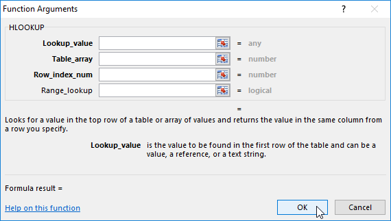
The HLOOKUP function in excel searches for a value in a table horizontally. HLOOKUP looks for a value in the top row of a specified table, or array, and then returns the corresponding value in a lower row, based on how many rows you specify. It’s identical to a VLOOKUP but works horizontally instead of vertically!
Syntax
=HLOOKUP(lookup_value,table_array,row_index_num,[range_lookup])
Parameters
- lookup_value – Again, this is the value we are searching for in our table_array.
- table_array – This is the row range in which we are looking for our lookup_value. This can be an entire row, a fixed range, a table range or a named range.
- row_index_num – This numerical value represents how many rows you want the formula to look from your table_array.
- range_lookup – This is an optional parameter that returns an exact match when FALSE is used and an approximate match or closest match when TRUE is used.
Example
In this example, we are looking for the author of a particular subject. We look up C2 and ask HLOOKUP to return the author from row three.
4. XLOOKUP
The XLOOKUP function was introduced as an improvement over the older functions like LOOKUP, VLOOKUP, HLOOKUP. You can only access the XLOOKUP function if you have Microsoft 365 (previously Office 365), or Microsoft Excel 2021 or later.
XLOOKUP is awesome, and a big improvement on the VLOOKUP, LOOKUP and HLOOKUP options because it can look up data anywhere in a table_array or lookup_range. VLOOKUP is restricting as it can only look for data from left to right, and HLOOKUP can only look for data from top to bottom. XLOOKUP makes looking up in any direction possible!
Syntax
=XLOOKUP(lookup_value, lookup_array, return_array, [if_not_found], [match_mode], [search_mode])
Parameters
- lookup_value – This is the value we are looking for in our lookup_array.
- lookup_array – This is the table range where we search for our lookup_value.
- return_array – This is the array that we want a return from. We’re asking XLOOKUP to match the value in the lookup_array and return the corresponding value in the return_array.
- if_not_found – This is an optional parameter. It dictates what we want XLOOKUP to return if there is no match. If it is not specified and no match is found, it generates a N/A error.
match_mode and search_mode extend the capabilities of XLOOKUP and allow you to add options to return the next smaller items or perform a return search. The uses here are broad, so we’ll cover how to use them in an article dedicated to XLOOKUP!
Example
In this example, we’re looking up the first name of someone in column B, based on their last name in column C. XLOOKUP allows us to look vertically from right to left in this instance. Something not possible with a VLOOKUP!
5. INDEX and MATCH
INDEX and MATCH combined are two of the most valuable functions in Excel for performing more advanced lookups. For example, you can use INDEX MATCH to perform horizontal and vertical lookups. If you want to be a master in Excel, learning INDEX and MATCH is a must.
INDEX MATCH is also available on most versions of Excel, unlike XLOOKUP. INDEX and MATCH are two separate functions that you can combine to achieve a look-up effect. Let’s take a look at them separately before combining them.
INDEX
The INDEX function returns a value based on the table_range specified.
Syntax
=INDEX(array,row_number)
Parameters
- array – This is the lookup range where the value is present. It’s where we want the formula to look.
- row_number – This is the row number from the starting index.
Example
In this example, we are looking at range B1 to B4 and asking Excel to return the value from the third row. In this case, cell B3.
The INDEX function can also return a value from two or more columns. In this instance, you have to include the row index and the column index.
=INDEX(array,row_number,[col_number])
MATCH
The MATCH function finds the position of a value in a given range and returns that value. It searches for a value both horizontally and vertically.
Syntax
=MATCH(lookup_value,lookup_array)
Parameters
- lookup_value – Explicitly mention the value here. If it is a text, enclose it in double-quotes.
- lookup_array – This is the lookup range.
Example 1
In this example, we ask Excel to look for the word “Grapes” in the range B2 to B5. “Grapes” is in the fourth row, so MATCH returns 4.
Example 2
If the exact value you are looking for is inside the formula, enclose it within double quotes. Otherwise, you can refer to a cell reference.
In this example, we refer to cell B8 as our lookup_value to complete our MATCH.
INDEX and MATCH Combined
You can use the MATCH function in combination with the INDEX function. When used together, you nest (embed) the MATCH function within an INDEX formula so that the MATCH element looks up which row the INDEX function should index.
Syntax
=INDEX(array,MATCH(lookup_value,lookup_array,0))
If that doesn’t make sense, here’s an example to help!
Example
In this example, we index the range D2 to D5 and then deploy our MATCH function to look up where within the range A2:A5 the value in C7 is. In this case, it’s looking up the value ’23’. This combination of INDEX and MATCH returns the adjacent value in column D for us – 15,000.
Frequently Asked Questions
1. How do you differentiate between VLOOKUP and LOOKUP?
The simplest difference between VLOOKUP and LOOKUP is the cross-functionality that LOOKUP has. VLOOKUP is limited to vertical lookups.
2. How do you define a LOOKUP Vector?
A LOOKUP Vector is used to look up a value in a one row/range area (Vector) and returns it from the exact position in a second one-row or one-column range.
3. How is XLOOKUP better than the INDEX_MATCH function in Excel?
The problem with the INDEX-MATCH function is that the formula is long and complex, whereas the XLOOKUP function has a simple syntax.
Wrapping Up
This guide explains what Lookup Functions do and walks you through the most common Lookups available.
We started with the basic LOOKUP function and then walked you through VLOOKUP and HLOOKUP.
LOOKUP, VLOOKUP and HLOOKUP all have limitations. So, we looked at some alternatives in the form of XLOOKUP and INDEX MATCH.
In summary, if you need to use a Lookup and have the option to use XLOOKUP, we recommend sticking with that. It’s more flexible than the other Lookup functions and less complicated than INDEX MATCH. XLOOKUP also allows you to add many additional conditions, making it far more valuable as your lookups become more complex.
If you enjoyed this article and are looking to take your Excel skills to the next level Academy of Learning offers world class courses in Excel and other Microsoft applications. Not sure if you’re ready to take the next step? Check out our article on 3 reasons to learn Microsoft Office, Professionally.

Introduction to LOOKUP Function in Excel
The Lookup function in Excel finds a specific value in a table or spreadsheet and shows you the related information in its adjacent cells in the same row. For example, if you want to search for the number 5 in a table, you could use the Lookup function to return the other information in the same row or column as 5.
The LOOKUP function is a built-in worksheet function in Microsoft Excel. It is available in Lookup & References under the Formula tab.
Syntax of Excel LOOKUP Function
The LOOKUP function in Excel is of two types: Vector and Array
#1 Vector form
The vector form of the LOOKUP function is useful for searching for a specific value in one row or column and returning a value from the same location in another row or column. For instance, you have a list of students with their names in one column and grades in another, and you want to find a grade for a particular student. The vector form of the LOOKUP function in Excel will search the student’s name and then display their grade from the same row.
If you know the row or column range where the search value is present, you can use this form of the LOOKUP function to get the value from that row or column.
Syntax: =LOOKUP(lookup_value, lookup_vector, [result_vector])
- Lookup Value: (Required) It is the value that we want to search in one row or one column. It can be a text, number, cell reference, value, or name.
- Lookup Vector: (Required) It is the range of one row or one column where the lookup_value will be first searched. The value can be numbers, text, or reference values.
- Result Vector: (Optional) It is the range of a single row or column from where we want to fetch the required value. The size of the result_vector must be the same as that of the lookup vector.
#2 Array form
An array is a combination of values in rows and columns in the form of a table. The array form of the LOOKUP function search for a specific value in the first row or column and returns a value from the same region in the last row or column of the array. Use this array form only when the values you want to search are in the array’s first row or column.
Note: Vlookup & Hlookup is used instead of an array form because it has limited options.
Syntax =LOOKUP(lookup_value, array)
- Lookup _value: (Required) lookup_value in array form is the value the LOOKUP function searches for in an array.
- Array: (Required)It is the range of cells of multiple rows and columns, like a two-dimensional data (table), where you want to search the lookup_value.
Let’s learn the use of the LOOKUP Function in Excel
In the following section, you will learn how to use the Lookup function with the help of various examples. You will also learn to create a LOOKUP formula to find a value for specific criteria.
You can download this LOOKUP Function Excel Template here – LOOKUP Function Excel Template
Example #1
How to search for a value in a one-column range?
In this example, you will learn how to search for a specific value in one column range using the vector form of the lookup function.
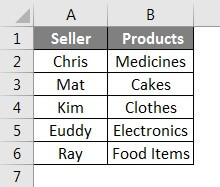
Consider the below table containing details of sellers and their products. You want to find out the product sold by Kim.
Solution:
Step 1: Click on Cell B10
Step 2: Enter the formula “=LOOKUP(B8,A2:A6,B2:B6)” as shown below.
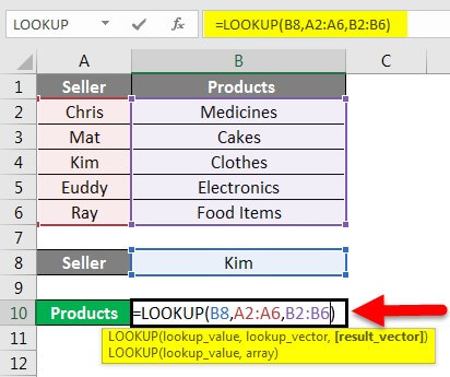
Step 3: Press “Enter”
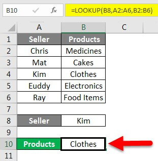
The result, “Clothes,” is displaced. Thus, Kim sold Clothes.
Explanation of the formula: “=Lookup(B8,A2:A6,B2:B6)”
This LOOKUP function searches the lookup_value, Cell B8 (Kim), in the lookup_vector, A2:A6, and returns the value in the same row from the result_vector, B2:B6. In simple terms, the value of Cell B8 is present in A4, and the function returns the value from the same position in another column, B4. The final output is Clothes.
Example #2
Let’s take another example to understand the vector form of the LOOKUP function.
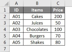
The below data consist of ID, Items, and their price, and you want to find out the price for ID A04. To search price, follow the steps of the solution.
Solution:
Step 1: Click on Cell B10
Step 2: Enter the formula “=LOOKUP(B8,A2:A6,C2:C6)” as shown below.
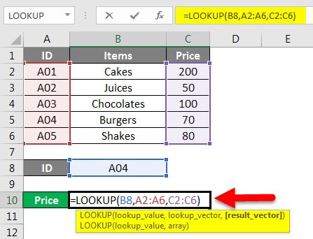
Step 3: Press “Enter” to get the result.
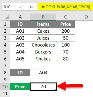
Output 70 is displayed as shown below. Hence, the price of ID A04 is 70.
Explanation of the formula: “=LOOKUP(B8,A2:A6,C2:C6)”
Here the lookup_value is A04; the lookup_vector is A2:A6, and the result_vector is C2:C6. The lookup_value, A04, is first searched in the range of lookup_vector (A2 to A6). The look_up value is in A5; now, the function returns the value in the same row from the result_vector range (B2:B6), i.e., B5. Thus, the output of the given formula is 70.
Example #3
How to search for a value in a one-row range?
In the above two examples, you have learned to use the vector form of the function to search for value in a single column. In this example, you will learn to search for value in a one-row range.
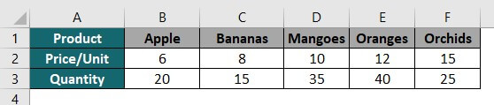
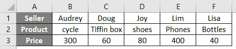
Consider the below table of products and their quantity arranged in a row. Now, you want to find the number of apples.
Solution:
Step 1: Click on Cell B7
Step 2: Enter the formula “LOOKUP(B5,B1:F1,B3:F3)” as shown below.
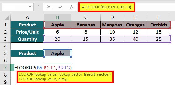
Step 3: Press “Enter” to get the desired result.
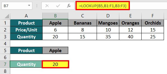
Output 20 is displaced in Cell B7. Thus, the quantity of apples is 20.
Example #4
How to search value using the array form?
In all the above examples, we have used the vector form of the LOOKUP function. In this example, we will use the array form.
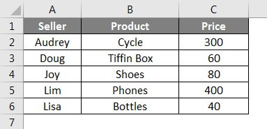
For instance, you have the below data and want to know the price of the product sold by Doug.
Solution:
Step 1: Click on Cell B9
Step 2: Enter the formula “=LOOKUP(B8,Al:C6)”, as shown below.
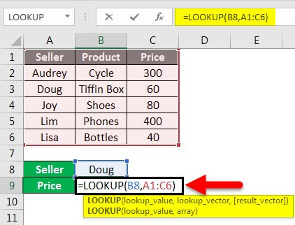
Step 3: Press “Enter” to see the result.
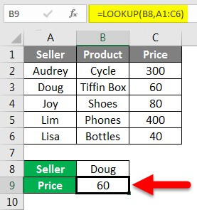
The result of the formula is 60. Thus, the price of the product sold by Doug is 60.
Explanation of the formula: “=LOOKUP(B8, A1:C6)”
Here, the lookup_value is B8, and the array range is A1: C6. The formula will search for the value of Cell B8 from Cell A1 to Cell C6 and returns the value corresponding to Cell B8.
Example #5
How to find a value in the last non-blank cell in a column?
In this example, you will learn to retrieve the last entry data, i.e., the last non-blank cell in a column, using the vector form of the LOOKUP function.
The syntax for retrieving the last value of a specific column is:
=Lookup(2,1/(column<>””), column)
Consider the below example. You need to find out the last entry in this table.

Solution:
Step 1: Click on Cell B8
Step 2: Enter the formula “=LOOKUP(2,1/(A2:A6<>””),A2:A6)” and press ”Enter”.

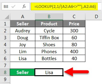
The output of the formula is Lisa. Thus, the last entry data in column A is Lisa.
Similarly, you can also find the last entry in the product and price columns. Enter the formula shown in the below image to get the desired result.
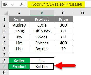
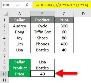
So, the last entry in column product is Bottles, and in price is 40.
Note: You must mention the column in the formula where you want to retrieve the last data entry.
Example #6
How to find a value in the last non-blank cell in a row?
In the previous example, you have learned to find the last entry in a specific column using the Lookup function. Here, you will learn to find the last entry in a particular row.
The syntax for retrieving the last value of a specific row is:
“= Lookup(2,1/(Row<>””),Row)”
In the data below, you have to find the last entry data in the Seller row.
Solution: Enter the formula=”LOOKUP(2,1/(B1:F1<>””),B1:F1)”lin the desired cell and press “Enter”.
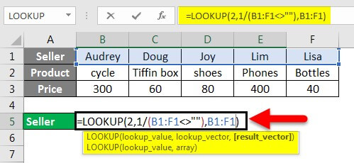
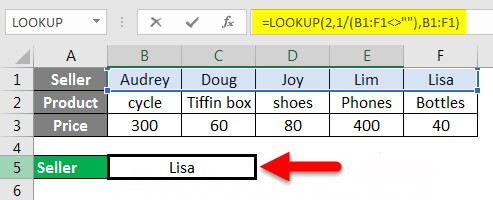
Result: The last entry in Seller Row is Lisa.
Things to Consider
#1 While Using the Vector Form of the LOOKUP Function
- The LOOKUP function with a result_vector provided will check for the lookup_value in the lookup_vector range and return the corresponding value from the result_vector.
- Without a result_vector, it will return the result value found from the lookup_vector.
- If the lookup_value cannot be found, the function returns the next smallest value or equal to the lookup_value.
- If the lookup_value is less than the lowest value in the lookup_vector, the function will display the #N/A error.
- The function will return the last value in the range if the lookup value is greater than each value in the lookup vector.
- If it cannot find the exact lookup_value, it searches for the next highest value that is lower than or equal to the lookup_value.
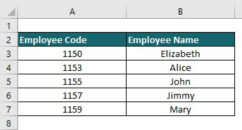
Let us learn about the above conditions through an example. The below data contains details of employee codes and their name.
Note: The data should be in ascending order.
|
Formula |
Description |
Result |
| =LOOKUP(1150,A3:A7,B3:B7) | The Lookup function finds the exact match of the lookup_value in column A. | Elizabeth |
| =LOOKUP(1156,A3:A7,B3:B7) | The function looks for the nearest value for 1156 and returns the value of 1157 | John |
| =LOOKUP(1151,A3:A7,B3:B7) | The function looks for the nearest value for 1151 and returns the value of 1150 | Elizabeth |
| =LOOKUP(1124,A3:A7,B3:B7) | lookup_value is smaller than all values present in A3:A7. | #N/A |
| =LOOKUP(0,A3:A7,B3:B7) | The function looks for 0 and returns an error because 0 is less than the smallest value, 1150. | #N/A |
| =LOOKUP(1162,A3:A7,B3:B7) | The function looks up for value 1162 and returns the last value from column A. | Mary |
#2 While Using the Array Form of the LOOKUP Function
- If the array range has multiple columns than rows (broader than taller), then the LOOKUP function will look for the lookup_value in the first row of the array (like HLOOKUP).
- If the array range has multiple rows than columns (taller than broader) or an equal number of rows and columns, then the LOOKUP function will look for the lookup_value in the first column (like VLOOKUP).
- In both cases, the LOOKUP function will return the very last value in the row or column of the array.
Essential Notes
- Sort the values in the lookup vector and result vector in ascending order, e., from A to Z if the values are in text and smallest to biggest if they are in numeric form.
- The LOOKUP function in Excel may provide incorrect results or errors if the data is unsorted.
- The LOOKUP function is not case-sensitive. It does not distinguish between text written in uppercase and lowercase.
- The lookup_vector and result_vector should be the same size when using the vector form of the LOOKUP function.
Frequently Asked Questions(FAQs)
Q1. What is the formula for lookup in Excel?
There are two types of lookup formulas in Excel.
- Vector form: The formula for the vector form of the lookup function is “=LOOKUP(lookup_value, lookup_vector, [result_vector])”
- Array form: The formula for the array form of the lookup function is “=LOOKUP(lookup_value, array)”
Q2. Why do we use lookup in Excel?
Excel’s lookup function is useful for finding a specific record, closest match, or corresponding value to a given value.
Recommended Articles
This article is a tutorial for the LOOKUP Function in Excel. We have covered how to use the LOOKUP function for different conditions in Excel, practical examples, and a downloadable Excel template. You might also read our other recommended articles:
- Goal Seek in Excel
- Excel Match Function
- VLOOKUP Function in EXCEL
- Scrollbar in Excel
The functions VLOOKUP and HLOOKUP among Excel users are very popular. The first function is used for vertical analysis, comparison. That is, it is used when the information is concentrated in columns.
HLOOKUP, respectively, is used for horizontal analysis. Inasmuch as there are rarely more rows in tables than columns, this function is rarely called.
The syntax of the VLOOKUP and HLOOKUP functions
The functions have 4 arguments:
- Lookup value: WHAT we are looking for – the desired parameter (numbers and / or text) or a reference to the cell with the desired value;
- Table array: WHERE we are looking for – an array of data where the search will be performed (for VLOOKUP – the searching of the value is carried out in the FIRST column of the table, for the HLOOKUP – from the FIRST line);
- Row index number: The NUMBER of the column / row – where exactly the corresponding value is returned (1 – from the first column or the first line, 2 – from the second one, etc.).
- Range lookup: The INTERVAL VIEW – the exact or approximate value should be found by the function (FALSE / 0 – the exact value, TRUE / 1 / not specified – the approximate value).
Attention! If the values in the range are sorted in ascending order (or alphabetically), we specify TRUE / 1. Otherwise – there is FALSE / 0.
How to use the VLOOKUP function in Excel: examples
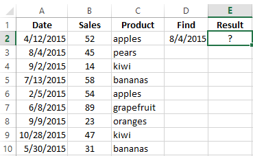
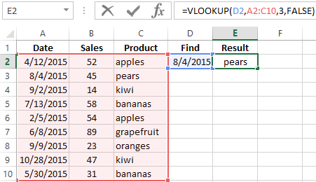
For the educational purposes, let’s take the table with the data:
| Formula | Description |
| =VLOOKUP(D2,A2:C10,3,FALSE) | The function searches for the value of the cell F5 in the range A2:C10 and returns the value of the cell F5, that was found in the column 3, the exact match. |
 |
|
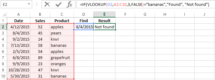
| =IF(VLOOKUP(D2,A$2:C$10,3,FALSE)=»bananas»,»Found», «Not found») | We need to find out whether bananas were sold 04. 08. 15. If bananas sold, the word «Found» appears in the corresponding cell. If bananas weren`t sold – «Not found». |
 |
|
| =IF(VLOOKUP(D2,A2:C10,3,FALSE)=»pears»,»Found», «Not found») | If the «bananas» are changed to «pears», the result will be «Found» |
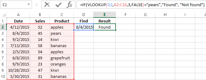 |
|
| =IFERROR(VLOOKUP(D2,A2:C10,3,FALSE),0) | When the VLOOKUP function can not find a value, it gives an error message # N/A. To avoid this, we use the function IFERROR. |
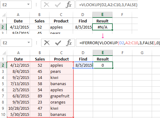 We will find out whether there were sales 08.05.15 |
|
| =VLOOKUP(A2,[employees.xlsx]Sheet1!A2:B10,2,FALSE) | If it`s necessary to implement for the search value in the another Excel workbook, then when filling out the «table» argument, we go to another workbook and select the desired range with the data. |
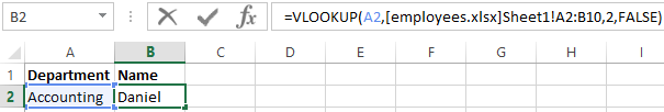 We wanted to know who worked 06. 08.15. |
|
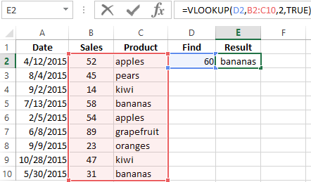
| =VLOOKUP(D2,B2:C10,2,TRUE) | The searching of the approximate value. |
 |
It is important:
- The VLOOKUP function always searches for data in the leftmost column of the table with values.
- The register is not taken into account: small and large letters for Excel are the same.
- If the sought after is less than the minimum value in the array, the program will return the error # N/D.
- If you set the column number to 0, the function will show #VALUE. If the third argument is greater than the number of columns in the table — #REFERENCE.
- To copy the correct array, we apply to the absolute references (F4 key).
How to use by the HLOOKUP function in Excel: examples
For educational purposes, let`s take the following table:
| Formula | Description |
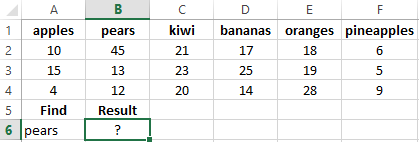
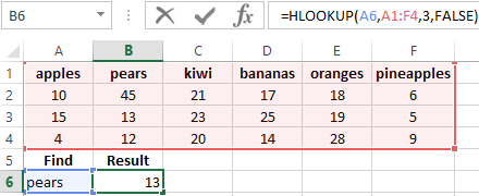
| =HLOOKUP(A6,A1:F4,3,FALSE) | Find the value of the cell |16 and return of the value from the third row of the same column. |
 |
The application of HLOOKUP in practice is limited, inasmuch as the horizontal representation of the information is used very rarely.
The symbols of substitution in VLOOKUP and HLOOKUP functions
It happens that the user does not remember the exact name. By specifying the desired value, he can apply the wildcard characters:
- «?» – replaces any character in text or digital information;
- «*» – for replacing any sequence of characters.
- Let`s find the text that begins or ends with a certain set of characters. For example we need to find the name of the company. We forgot it, but remember that it starts with Kol. The problem will be solved by the following formula:
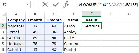
- We need to find the name of the company that ends with – «uda». The following formula will help:
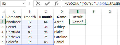
- Let`s find a company which name begins with «Ce» and ends with «sef». The formula of the VLOOKUP will look like this:
When the problems with memory are eliminated, you can work with data using all of the same functions.
How to compare sheets with the helping of VLOOKUP and HLOOKUP?
We have data about sales for January and February. These tables need to be compared using the formulas VLOOKUP and HLOOKUP. For clarity, we’ll put them in one sheet for now, but we will work in conditions when the ranges are in different sheets.
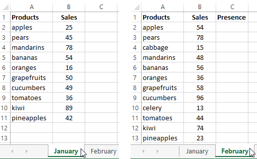
How can I compare sheets using VLOOKUP in Excel?
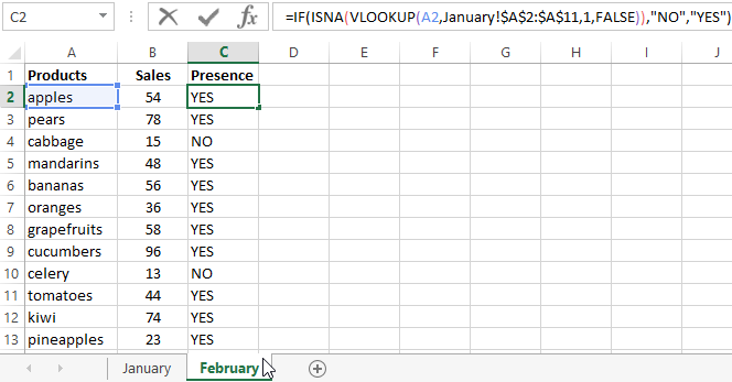
Let`s solve the problem 1: we compare the names of goods in January and February. Inasmuch as there are more of them in February, we will enter the formula on the «February» sheet.
Let`s solve the problem 2: we compare the sales by positions in January and February. We use the following formula:
How can I compare sheets with HLOOKUP in Excel?
To demonstrate the action of the HLOOKUP function, we take two «horizontal» tables, located on different sheets.
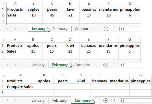
The task – is to compare sales by positions for January and February.
We create the new «Compare» sheet. This is not the obligatory condition. You can compare the data and display the difference on any sheet («January» or «February»).
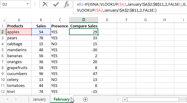
The formula:
The result:
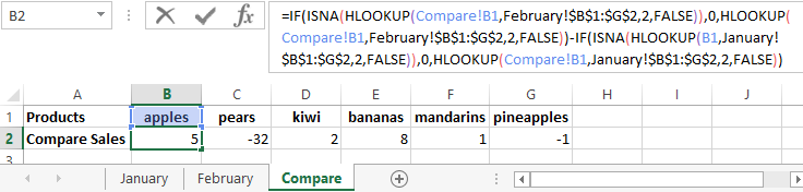
Let analyze the parts of the formula:
«Half» up to the sign «-»:
=IF(ISNA(HLOOKUP(Compare!B1,February!$B$1:$G$2,2,FALSE)),0,HLOOKUP(
Compare!B1,February!$B$1:$G$2,2,FALSE))-
The desired value – is the first cell in the table for comparison. The analyzed range – is the table with sales for February. The HLOOKUP function «takes» data from the second line in «accurate» reproduction.
After the «-» sign:
-IF(ISNA(HLOOKUP(B1,January!
$B$1:$G$2,2,FALSE)),0,HLOOKUP(Compare!B1,January!$B$1:$G$2,2,FALSE))
There are all the same in addition to the range. Here we take the table with sales for January.
Download example functions VLOOKUP and HLOOKUP
When we enter a formula, Excel prompts about: what the argument you need to enter now.
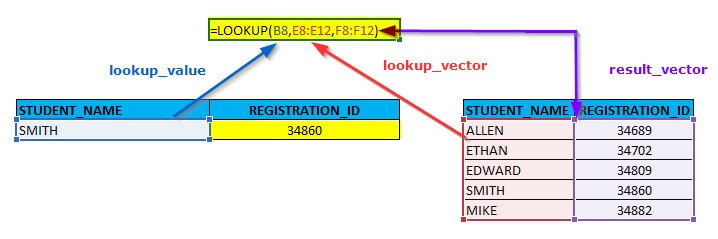
Use the LOOKUP function to look up a value in a one-column or one-row range, and retrieve a value from the same position in another one-column or one-row range. The lookup function has two forms, vector and array. The majority of this article describes the vector form, but the last example below illustrates the array form.
The LOOKUP function accepts three arguments: lookup_value, lookup_vector, and result_vector. The first argument, lookup_value, is the value to look for. The second argument, lookup_vector, is a one-row, or one-column range to search. LOOKUP assumes that lookup_vector is sorted in ascending order. The third argument, result_vector, is a one-row, or one-column range of results. Result_vector is optional. When result_vector is provided, LOOKUP locates a match in the lookup_vector, and returns the corresponding value from result_vector. If result_vector is not provided, LOOKUP returns the value of the match found in lookup_vector.
LOOKUP has default behaviors that make it useful when solving certain problems. For example, LOOKUP can be used to retrieve an approximate-matched value instead of a position and to find the last value in a row or column. LOOKUP assumes that values in lookup_vector are sorted in ascending order and always performs an approximate match. When LOOKUP can’t find a match, it will match the next smallest value.
Example #1 — basic usage
In the example shown above, the formula in cell F5 returns the value of the match found in column B. Note that result_vector is not provided:
=LOOKUP(F4,B5:B9) // returns match in level
The formula in cell F6 returns the corresponding Tier value from column C. Notice in this case, both lookup_vector and result_vector are provided:
=LOOKUP(F4,B5:B9,C5:C9) // returns corresponding tier
In both formulas, LOOKUP automatically performs an approximate match and it is therefore important that lookup_vector is sorted in ascending order.
Example #2 — last non-empty cell
LOOKUP can be used to get the value of the last filled (non-empty) cell in a column. In the screen below, the formula in F6 is:
=LOOKUP(2,1/(B:B<>""),B:B)

Note the use of a full column reference. This is not an intuitive formula, but it works well. The key to understanding this formula is to recognize that the lookup_value of 2 is deliberately larger than any values that will appear in the lookup_vector. Detailed explanation here.
Example #3 — latest price
Similar to the above example, the lookup function can be used to look up the latest price in data sorted in ascending order by date. In the screen below, the formula in G5 is:
=LOOKUP(2,1/(item=F5),price)
where item (B5:B12) and price (D5:D12) are named ranges.

When lookup_value is greater than all values in lookup_array, default behavior is to «fall back» to the previous value. This formula exploits this behavior by creating an array that contains only 1s and errors, then deliberately looking for the value 2, which will never be found. More details here.
Example #4 — array form
The LOOKUP function has an array form as well. In the array configuration, LOOKUP takes just two arguments: the lookup_value, and a single two-dimensional array:
LOOKUP(lookup_value, array) // array form
In the array form, LOOKUP evaluates the array and automatically changes behavior based on the array dimensions. If the array is wider than tall, LOOKUP looks for the lookup value in the first row of the array (like HLOOKUP). If the array is taller than wide (or square), LOOKUP looks for the lookup value in the first column (like VLOOKUP). In either case, LOOKUP returns a value at the same position from the last row or column in the array. The example below shows how the array form works. The formula in F5 is configured to use a vertical array and the formula in F6 is configured to use a horizontal array:
=LOOKUP(E5,B5:C9) // vertical array
=LOOKUP(E6,C11:G12) // horizontal array

The vertical and horizontal arrays contain the same values; only the orientation is different.
Note: Microsoft discourages the use of the array form and suggests VLOOKUP and HLOOKUP as better options.
Notes
- LOOKUP assumes that lookup_vector is sorted in ascending order.
- When lookup_value can’t be found, LOOKUP will match the next smallest value.
- When lookup_value is greater than all values in lookup_vector, LOOKUP matches the last value.
- When lookup_value is less than the first value in lookup_vector, LOOKUP returns #N/A.
- Result_vector must be the same size as lookup_vector.
- LOOKUP is not case-sensitive