Excel for Microsoft 365 Excel for Microsoft 365 for Mac Excel for the web Excel 2021 Excel 2021 for Mac Excel 2019 Excel 2019 for Mac Excel 2016 Excel 2016 for Mac Excel 2013 Excel 2010 Excel 2007 Excel for Mac 2011 Excel Starter 2010 More…Less
Tip: Try using the new XLOOKUP function, an improved version of VLOOKUP that works in any direction and returns exact matches by default, making it easier and more convenient to use than its predecessor.
Use VLOOKUP when you need to find things in a table or a range by row. For example, look up a price of an automotive part by the part number, or find an employee name based on their employee ID.
In its simplest form, the VLOOKUP function says:
=VLOOKUP(What you want to look up, where you want to look for it, the column number in the range containing the value to return, return an Approximate or Exact match – indicated as 1/TRUE, or 0/FALSE).
Tip: The secret to VLOOKUP is to organize your data so that the value you look up (Fruit) is to the left of the return value (Amount) you want to find.
Use the VLOOKUP function to look up a value in a table.
Syntax
VLOOKUP (lookup_value, table_array, col_index_num, [range_lookup])
For example:
-
=VLOOKUP(A2,A10:C20,2,TRUE)
-
=VLOOKUP(«Fontana»,B2:E7,2,FALSE)
-
=VLOOKUP(A2,’Client Details’!A:F,3,FALSE)
|
Argument name |
Description |
|---|---|
|
lookup_value (required) |
The value you want to look up. The value you want to look up must be in the first column of the range of cells you specify in the table_array argument. For example, if table-array spans cells B2:D7, then your lookup_value must be in column B.
|
|
table_array (required) |
The range of cells in which the VLOOKUP will search for the lookup_value and the return value. You can use a named range or a table, and you can use names in the argument instead of cell references. The first column in the cell range must contain the lookup_value. The cell range also needs to include the return value you want to find. Learn how to select ranges in a worksheet. |
|
col_index_num (required) |
The column number (starting with 1 for the left-most column of table_array) that contains the return value. |
|
range_lookup (optional) |
A logical value that specifies whether you want VLOOKUP to find an approximate or an exact match:
|
How to get started
There are four pieces of information that you will need in order to build the VLOOKUP syntax:
-
The value you want to look up, also called the lookup value.
-
The range where the lookup value is located. Remember that the lookup value should always be in the first column in the range for VLOOKUP to work correctly. For example, if your lookup value is in cell C2 then your range should start with C.
-
The column number in the range that contains the return value. For example, if you specify B2:D11 as the range, you should count B as the first column, C as the second, and so on.
-
Optionally, you can specify TRUE if you want an approximate match or FALSE if you want an exact match of the return value. If you don’t specify anything, the default value will always be TRUE or approximate match.
Now put all of the above together as follows:
=VLOOKUP(lookup value, range containing the lookup value, the column number in the range containing the return value, Approximate match (TRUE) or Exact match (FALSE)).
Examples
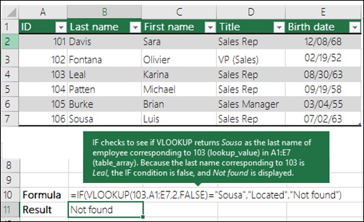
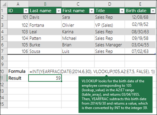
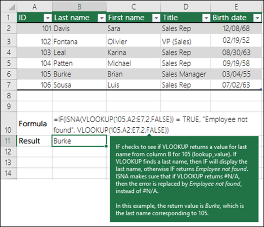
Here are a few examples of VLOOKUP:
Example 1
Example 2
Example 3
Example 4
Example 5
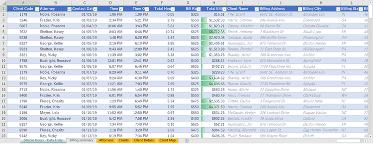
You can use VLOOKUP to combine multiple tables into one, as long as one of the tables has fields in common with all the others. This can be especially useful if you need to share a workbook with people who have older versions of Excel that don’t support data features with multiple tables as data sources — by combining the sources into one table and changing the data feature’s data source to the new table, the data feature can be used in older Excel versions (provided the data feature itself is supported by the older version).
|
|
Here, columns A-F and H have values or formulas that only use values on the worksheet, and the rest of the columns use VLOOKUP and the values of column A (Client Code) and column B (Attorney) to get data from other tables. |
-
Copy the table that has the common fields onto a new worksheet, and give it a name.
-
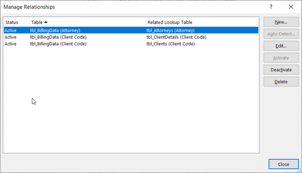
Click Data > Data Tools > Relationships to open the Manage Relationships dialog box.
-
For each listed relationship, note the following:
-
The field that links the tables (listed in parentheses in the dialog box). This is the lookup_value for your VLOOKUP formula.
-
The Related Lookup Table name. This is the table_array in your VLOOKUP formula.
-
The field (column) in the Related Lookup Table that has the data you want in your new column. This information is not shown in the Manage Relationships dialog — you’ll have to look at the Related Lookup Table to see which field you want to retrieve. You want to note the column number (A=1) — this is the col_index_num in your formula.
-
-
To add a field to the new table, enter your VLOOKUP formula in the first empty column using the information you gathered in step 3.
In our example, column G uses Attorney (the lookup_value) to get the Bill Rate data from the fourth column (col_index_num = 4) from the Attorneys worksheet table, tblAttorneys (the table_array), with the formula =VLOOKUP([@Attorney],tbl_Attorneys,4,FALSE).
The formula could also use a cell reference and a range reference. In our example, it would be =VLOOKUP(A2,’Attorneys’!A:D,4,FALSE).
-
Continue adding fields until you have all the fields that you need. If you are trying to prepare a workbook containing data features that use multiple tables, change the data source of the data feature to the new table.
|
Problem |
What went wrong |
|---|---|
|
Wrong value returned |
If range_lookup is TRUE or left out, the first column needs to be sorted alphabetically or numerically. If the first column isn’t sorted, the return value might be something you don’t expect. Either sort the first column, or use FALSE for an exact match. |
|
#N/A in cell |
For more information on resolving #N/A errors in VLOOKUP, see How to correct a #N/A error in the VLOOKUP function. |
|
#REF! in cell |
If col_index_num is greater than the number of columns in table-array, you’ll get the #REF! error value. For more information on resolving #REF! errors in VLOOKUP, see How to correct a #REF! error. |
|
#VALUE! in cell |
If the table_array is less than 1, you’ll get the #VALUE! error value. For more information on resolving #VALUE! errors in VLOOKUP, see How to correct a #VALUE! error in the VLOOKUP function. |
|
#NAME? in cell |
The #NAME? error value usually means that the formula is missing quotes. To look up a person’s name, make sure you use quotes around the name in the formula. For example, enter the name as «Fontana» in =VLOOKUP(«Fontana»,B2:E7,2,FALSE). For more information, see How to correct a #NAME! error. |
|
#SPILL! in cell |
This particular #SPILL! error usually means that your formula is relying on implicit intersection for the lookup value, and using an entire column as a reference. For example, =VLOOKUP(A:A,A:C,2,FALSE). You can resolve the issue by anchoring the lookup reference with the @ operator like this: =VLOOKUP(@A:A,A:C,2,FALSE). Alternatively, you can use the traditional VLOOKUP method and refer to a single cell instead of an entire column: =VLOOKUP(A2,A:C,2,FALSE). |
|
Do this |
Why |
|---|---|
|
Use absolute references for range_lookup |
Using absolute references allows you to fill-down a formula so that it always looks at the same exact lookup range. Learn how to use absolute cell references. |
|
Don’t store number or date values as text. |
When searching number or date values, be sure the data in the first column of table_array isn’t stored as text values. Otherwise, VLOOKUP might return an incorrect or unexpected value. |
|
Sort the first column |
Sort the first column of the table_array before using VLOOKUP when range_lookup is TRUE. |
|
Use wildcard characters |
If range_lookup is FALSE and lookup_value is text, you can use the wildcard characters—the question mark (?) and asterisk (*)—in lookup_value. A question mark matches any single character. An asterisk matches any sequence of characters. If you want to find an actual question mark or asterisk, type a tilde (~) in front of the character. For example, =VLOOKUP(«Fontan?»,B2:E7,2,FALSE) will search for all instances of Fontana with a last letter that could vary. |
|
Make sure your data doesn’t contain erroneous characters. |
When searching text values in the first column, make sure the data in the first column doesn’t have leading spaces, trailing spaces, inconsistent use of straight ( ‘ or » ) and curly ( ‘ or “) quotation marks, or nonprinting characters. In these cases, VLOOKUP might return an unexpected value. To get accurate results, try using the CLEAN function or the TRIM function to remove trailing spaces after table values in a cell. |
Need more help?
You can always ask an expert in the Excel Tech Community or get support in the Answers community.

See Also
XLOOKUP function
Video: When and how to use VLOOKUP
Quick Reference Card: VLOOKUP refresher
How to correct a #N/A error in the VLOOKUP function
Look up values with VLOOKUP, INDEX, or MATCH
HLOOKUP function
Need more help?
Want more options?
Explore subscription benefits, browse training courses, learn how to secure your device, and more.
Communities help you ask and answer questions, give feedback, and hear from experts with rich knowledge.
VLOOKUP is an Excel function to get data from a table organized vertically. Lookup values must appear in the first column of the table passed into VLOOKUP. VLOOKUP supports approximate and exact matching, and wildcards (* ?) for partial matches.
Vertical data | Column Numbers | Only looks right | Matching Modes | Exact Match | Approximate Match | First Match | Wildcard Match | Two-way Lookup | Multiple Criteria | #N/A Errors | Videos
Introduction
VLOOKUP is probably the most famous function in Excel, for reasons both good and bad. On the good side, VLOOKUP is easy to use and does something very useful. For new users in particular, it is immensely satisfying to watch VLOOKUP scan a table, find a match, and return a correct result. Using VLOOKUP successfully is a rite of passage for new Excel users.
On the bad side, VLOOKUP is limited and has dangerous defaults. Unlike INDEX and MATCH (or XLOOKUP), VLOOKUP needs a complete table with lookup values in the first column. This makes it hard to use VLOOKUP with multiple criteria. In addition, VLOOKUP’s default matching behavior makes it easy to get incorrect results. Fear not. The key to using VLOOKUP successfully is mastering the basics. Read on for a complete overview.
Arguments
VLOOKUP takes four arguments: lookup_value, table_array, column_index_num, and range_lookup. Lookup_value is the value to look for, and table_array is the range of vertical data to look inside. The first column of table_array must contain the lookup values to search. The column_index_num argument is the column number of the value to retrieve, where the first column of table_array is column 1. Finally, range_lookup controls match behavior. If range_lookup is TRUE, VLOOKUP will perform an approximate match. If range_lookup is FALSE, VLOOKUP will perform an exact match. Important: range_lookup is optional and defaults to TRUE, so VLOOKUP will perform an approximate match by default. See below for more information on matching.
V is for vertical
The purpose of VLOOKUP is to look up information in a table like this:
With the Order number in column B as the lookup_value, VLOOKUP can get the Cust. ID, Amount, Name, and State for any order. For example, to get the name for order 1004, the formula is:
=VLOOKUP(1004,B5:F9,4,FALSE) // returns "Sue Martin"
To look up horizontal data, you can use HLOOKUP, INDEX and MATCH, or XLOOKUP.
VLOOKUP is based on column numbers
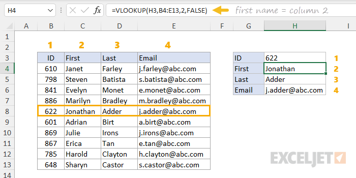
When you use VLOOKUP, imagine that every column in the table_array is numbered, starting from the left. To get a value from a given column, provide the number for column_index_num. For example, the column index to retrieve the first name below is 2:
By changing only column_index_num, you can look up columns 2, 3, and 4:
=VLOOKUP(H3,B4:E13,2,FALSE) // first name
=VLOOKUP(H3,B4:E13,3,FALSE) // last name
=VLOOKUP(H3,B4:E13,4,FALSE) // email address
Note: normally, we would use an absolute reference for H3 ($H$3) and B4:E13 ($B$4:$E$13) to prevent these from changing when the formula is copied. Above, the references are relative to make them easier to read.
VLOOKUP only looks right
VLOOKUP can only look to the right. In other words, you can only retrieve data to the right of the column that holds lookup values:
To look up values to the left, see INDEX and MATCH, or XLOOKUP.
Match modes
VLOOKUP has two modes of matching, exact and approximate, controlled by the fourth argument, range_lookup. The word «range» in this case refers to «range of values» – when range_lookup is TRUE, VLOOKUP will match a range of values rather than an exact value. A good example of this is using VLOOKUP to calculate grades. When range_lookup is FALSE, VLOOKUP performs an exact match, as in the example above.
Important: range_lookup is optional defaults to TRUE. This means approximate match mode is the default, which can be dangerous. Set range_lookup to FALSE to force exact matching:
=VLOOKUP(value,table,col_index) // approximate match (default)
=VLOOKUP(value,table,col_index,TRUE) // approximate match
=VLOOKUP(value,table,col_index,FALSE) // exact match
Tip: always supply a value for range_lookup as a reminder of expected behavior.
Note: You can also supply zero (0) for an exact match, and 1 for an approximate match.
Exact match example
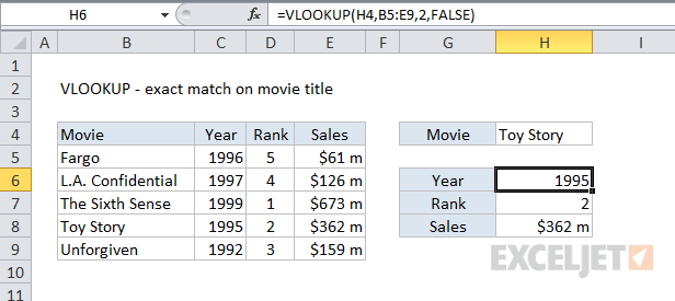
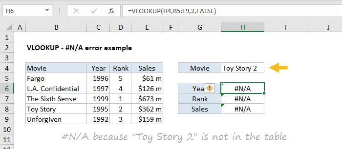
In most cases, you’ll probably want to use VLOOKUP in exact match mode. This makes sense when you have a unique key to use as a lookup value, for example, the movie title in this data:
The formula in H6 to find Year, based on an exact match of the movie title, is:
=VLOOKUP(H4,B5:E9,2,FALSE) // FALSE = exact match
Approximate match example
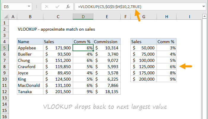
In some cases, you will need an approximate match lookup instead of an exact match lookup. For example, below we want to find the correct commission percentage in the range G5:H10 based on the sales amount in column C. In this example, we need to use VLOOKUP in approximate match mode, because in most cases an exact match will never be found. The VLOOKUP formula in D5 is configured to perform an approximate match by setting the last argument to TRUE:
=VLOOKUP(C5,$G$5:$H$10,2,TRUE) // TRUE = approximate match
VLOOKUP will scan values in column G for the lookup value. If an exact match is found, VLOOKUP will use it. If not, VLOOKUP will «step back» and match the previous row.
Note: The table_array must be sorted in ascending order by lookup value to use an approximate match. If table_array is not sorted by the first column in ascending order, VLOOKUP may return incorrect or unexpected results.
First match only
In the case of duplicate matching values, VLOOKUP will find the first match. In the screen below, VLOOKUP is configured to find the price for the color «Green». There are three rows with the color Green, and VLOOKUP returns the price in the first row, $17. The formula in cell F5 is:
=VLOOKUP(E5,B5:C11,2,FALSE) // returns 17
Tip: To retrieve multiple matches with a lookup operation, see the FILTER function.
Wildcard match
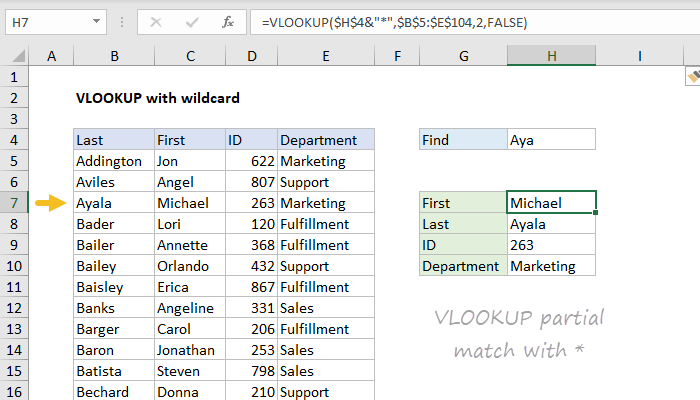
The VLOOKUP function supports wildcards, which makes it possible to perform a partial match on a lookup value. For instance, you can use VLOOKUP to retrieve information from a table with a partial lookup_value and wildcard. To use wildcards with VLOOKUP, you must use exact match mode by providing FALSE for range_lookup. In the screen below, the formula in H7 retrieves the first name, «Michael», after typing «Aya» into cell H4. Notice the asterisk (*) wildcard is concatenated to the lookup value inside the VLOOKUP formula:
=VLOOKUP($H$4&"*",$B$5:$E$104,2,FALSE)
Read a more detailed explanation here.
Two-way lookup
Inside the VLOOKUP function, column_index_num is normally hard-coded as a static number. However, you can create a dynamic column index by using the MATCH function to locate the needed column. This technique allows you to create a dynamic two-way lookup, matching on both rows and columns. In the screen below, VLOOKUP is configured to perform a lookup based on Name and Month like this:
=VLOOKUP(H4,B5:E13,MATCH(H5,B4:E4,0),0)
For more details, see this example.
Note: In general, INDEX and MATCH is a more flexible way to perform two-way lookups.
Multiple criteria
The VLOOKUP function does not handle multiple criteria natively. However, you can use a helper column to join multiple fields together and use these fields like multiple criteria inside VLOOKUP. In the example below, Column B is a helper column that concatenates first and last names together with this formula:
=C5&D5 // helper column
VLOOKUP is configured to do the same thing to create a lookup value. The formula in H6 is:
=VLOOKUP(H4&H5,B5:E13,4,0)
For details, see this example. For a more advanced, flexible approach, see this example.
Note: INDEX and MATCH and XLOOKUP are better for lookups based on multiple criteria.
VLOOKUP and #N/A errors
If you use VLOOKUP you will inevitably run into the #N/A error. The #N/A error means «not found». For example, in the screen below, the lookup value «Toy Story 2» does not exist in the lookup table, and all three VLOOKUP formulas return #N/A:
The #N/A error is useful because tells you something is wrong. The reason for #N/A might be:
- The lookup value does not exist in the table
- The lookup value is misspelled or contains extra space
- Match mode is exact, but should be approximate
- The table range is not entered correctly
- You are copying VLOOKUP, and the table reference is not locked
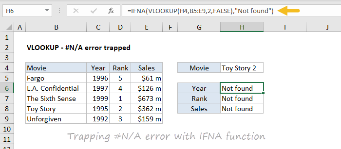
To «trap» the NA error and return a different value, you can use the IFNA function like this:
The formula in H6 is:
=IFNA(VLOOKUP(H4,B5:E9,2,FALSE),"Not found")
The message can be customized as desired. To return nothing (i.e. to display a blank result) when VLOOKUP returns #N/A you can use an empty string («») like this:
=IFNA(VLOOKUP(H4,B5:E9,2,FALSE),"") // no message
You can also use the IFERROR function to trap VLOOKUP #N/A errors. However, be careful with IFERROR, because it will catch any error, not just the #N/A error. Read more: VLOOKUP without #N/A errors
More about VLOOKUP
- VLOOKUP with multiple criteria (basic)
- VLOOKUP with multiple criteria (advanced)
- How to use VLOOKUP to merge tables
- 23 tips for using VLOOKUP
- More VLOOKUP examples and videos
- XLOOKUP vs VLOOKUP
Other notes
- VLOOKUP performs an approximate match by default.
- VLOOKUP is not case-sensitive.
- Range_lookup controls the match mode. FALSE = exact, TRUE = approximate (default).
- If range_lookup is omitted or TRUE or 1:
- VLOOKUP will match the nearest value less than the lookup_value.
- VLOOKUP will still use an exact match if one exists.
- The column 1 of table_array must be sorted in ascending order.
- If range_lookup is FALSE or zero:
- VLOOKUP performs an exact match.
- Column 1 of table_array does not need to be sorted.
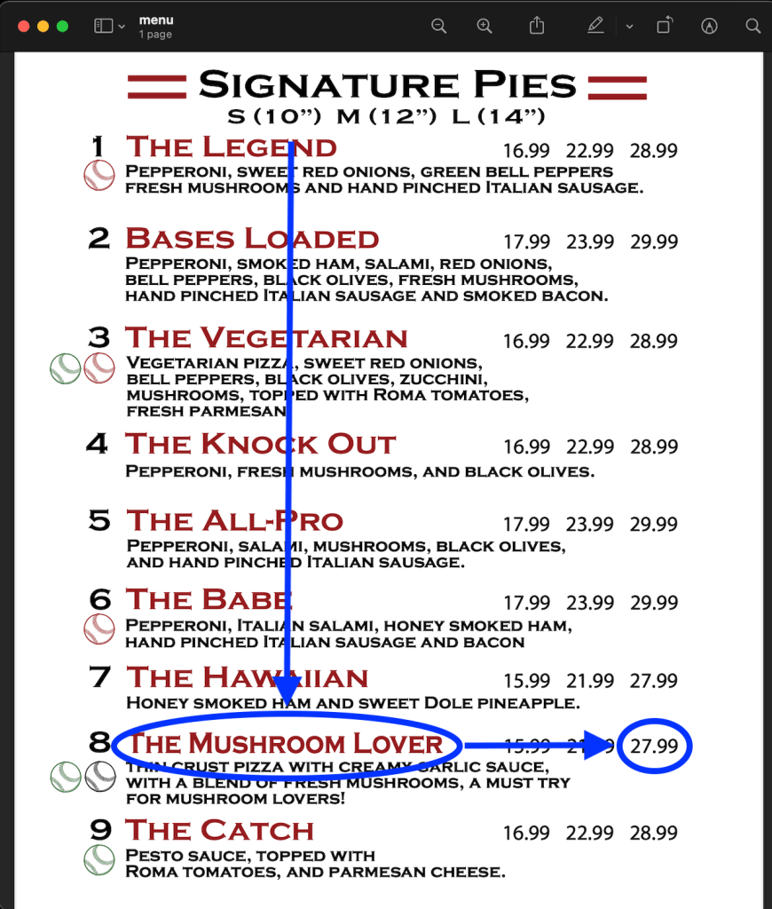
When you learn the price of the menu below, first your eyes will look up vertically to find your favorite pie, such as The Mushroom Lover. Then your vision slides to the right to find the price for the L size – $27.99.
You’ve just done a vertical lookup, or vlookup. For this purpose, spreadsheet apps including Excel usually provide a specified function called VLOOKUP. In this article, we’ll explore how you can use the Excel VLOOKUP function, check out a few examples, and learn how to troubleshoot it.
What is VLOOKUP in Excel
VLOOKUP stands for vertical lookup. It is a function in Excel that searches vertically a specified value in a column to return a matching value, or values in the same row from different columns.
VLOOKUP syntax in Excel
=VLOOKUP("lookup_value",lookup_range, column_number, [match])"lookup_value"is the value you want to look up vertically. Quotes are not used if you reference a cell as a lookup value.lookup_rangeis the data range where you’ll search for thelookup_valueand the matching value.column_numberis the number of the column in thelookup_range, which contains the matching value to return. For example, if your range is D7:G18, D is the first column, E is the second one, and so on.[match]is the optional parameter to choose either closest or exact match. To return the closest match, specify TRUE; to return an exact match, specify FALSE. The closest match (TRUE) is set by default.
How to VLOOKUP in Excel – formula example
We have the following dataset with the details of courses:
Let’s search for the day when College Writing III is scheduled. Here is the VLOOKUP formula to do this:
=VLOOKUP(A10,A2:H12,6,FALSE)
A10– the lookup_value “College Writing III“A2:H12– the lookup_range6– the column number to return the matching value fromFALSE– the exact match to return
The result of the schedule for College Writing III is Thursday. And here is how the logic of this VLOOKUP formula looks:
- Excel searches the value of
A10(College Writing III) in the lookup column (A2:A12). - If the value is found, Excel moves across the row to column number 6 of the specified data lookup range (
A2:H12). Column A is the first column in the lookup range, because column A contains the lookup value. - As the formula is set to FALSE (to find the exact match) then the return value is Thursday (you can see the result in A14).
What you should know about VLOOKUP in Excel
- The VLOOKUP function executes a case-insensitive lookup.
- Excel VLOOKUP returns a #N/A if the
lookup_valueis not able to be found inside thelookup_range. - Excel VLOOKUP returns a
#VALUE!error if the value ofcolumn_numberis less than 1. - Excel VLOOKUP returns a
#REF!error if the value of column number is greater than the number of columns in thelookup_range. - The closest match (TRUE) is specified by default.
How to pull your data to Excel for vertical lookup
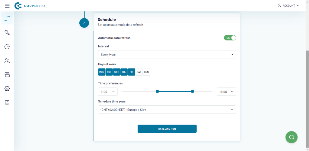
The example above is basic for you to understand the logic of the Excel VLOOKUP function. Your cases probably will be more advanced for the data that you can import from different sources to Excel. How? Coupler.io, an integration solution, is designed to export data from multiple apps and sources to Excel or Google Sheets or BigQuery on a schedule. You just need to sign up to Coupler.io and:
- Select and set up a source:
Check out the HubSpot to Excel integration.
- Select and set up a destination (in our case – Microsoft Excel)
- Set up a schedule (optionally) if you want to automate export of your data on a custom schedule.
With your data exported from BigQuery, HubSpot, Xero, etc. to Microsoft Excel, you can easily vlookup it.
How to use VLOOKUP in Excel
There are two ways to access VLOOKUP in Excel – you can use the VLOOKUP formula in the formula bar or access it through the menu bar.
Type directly into the cell
In the example above, we used VLOOKUP in Excel this way. You need to click in the cell where you want the answer to appear, then put the cursor on Formula Bar. Type the VLOOKUP formula and all its parameters directly into the formula bar:
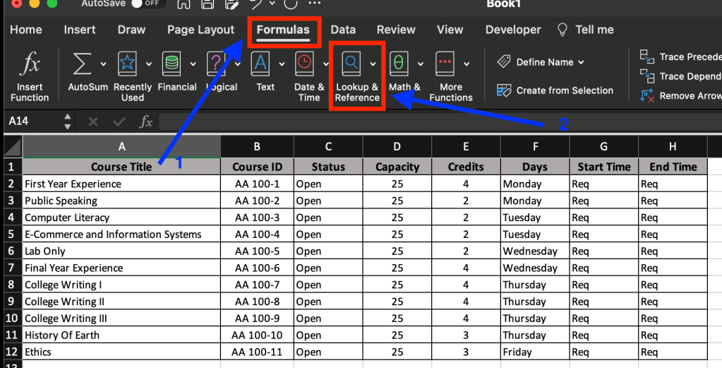
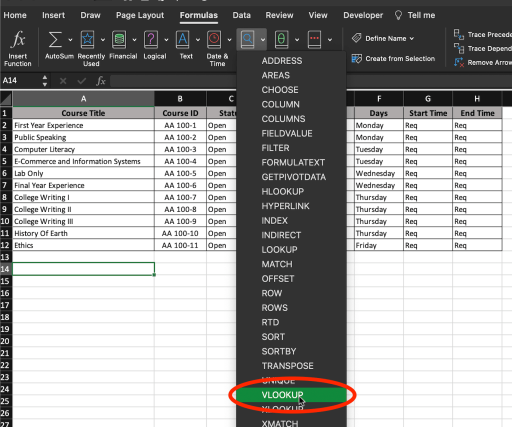
- In the menu bar, select the Formulas tab, then select Lookup & Reference.
- An alphabetical menu will drop down – choose VLOOKUP.
- On your right side, the Formula Builder will appear.
- Fill each box in the Formula Builder as your VLOOKUP formula parameters, then click Done.
Here is how it will look for our Vlookup formula example:
The result is the same – Thursday. So it is up to you which way is easier for you to use the VLOOKUP function 🙂
Excel VLOOKUP for an array
In the Excel VLOOKUP, you can use an array as a lookup_value. This will let you search the matches for multiple values.
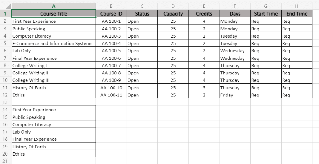
Let’s take the data set from above and vertically look up for the days when the values from the range A14:A20 are scheduled.
Here is the VLOOKUP formula to do this:
=VLOOKUP(A14:A20,Sheet1!A2:H12,6,FALSE)
A14:A20– the lookup arraySheet1!A2:H12– the lookup range6– the column number to return the matching value fromFALSE– the exact match to return
Excel vlookup cases
Check out the following specific cases of how to vlookup data in Excel:
- How to VLOOKUP for multiple matches
- How to VLOOKUP for two values
- How to VLOOKUP for multiple criteria
- How to compare two columns in Excel using VLOOKUP
- How to VLOOKUP another sheet in Excel
- How to vlookup another workbook/spreadsheet in Excel
- How to vlookup multiple columns in Excel
- Excel SUMIF with VLOOKUP
Excel reverse VLOOKUP
VLOOKUP in Excel can only look up the matching values from left to right.
And what if your data set look like this and you need to look up values from right to left:
Unfortunately, in this case you can’t use VLOOKUP, but the Excel XLOOKUP function will do the job.
Note: The XLOOKUP function is only available in Excel Online and Microsoft 365.
Reverse VLOOKUP syntax
=XLOOKUP("lookup_value", lookup_array, return_array, "[if_not_found]", [match_mode], [search_mode])lookup_valueis the value you want to look up vertically.lookup_arrayis the data array to search thelookup_value.return_arrayis the data array to return the matching value.[if_not_found]is the optional parameter to return a specified text if thelookup_valuehas not been found.[match_mode]is the optional parameter to choose the match mode:0– Exact match (default)-1– If the exact match is not found, the next smallest item is returned.1– If the exact match is not found, the next largest item is returned.2– A wildcard match where*,?, and~have special meaning.
[search_mode]is the optional parameter to choose the search mode:1– Search starting at the first item (default).-1– Search starting at the last item.2– Binary search that relies onlookup_arraybeing sorted in ascending order. If not sorted, invalid results will be returned.-2– Binary search that relies onlookup_arraybeing sorted in descending order. If not sorted, invalid results will be returned.
Reverse VLOOKUP formula example
Let’s search for the day when Lab Only is scheduled. Here is the XLOOKUP formula to do this:
=XLOOKUP("Lab Only",H2:H12,E2:E12,"Not found")
"Lab Only"– the lookup value.H2:H12– the data array to search for the lookup valueE2:E12– the data array to return the matching value."Not found"– the text to return if the lookup value has not been found.
Another way to do a reverse vlookup is using a combination of the INDEX and MATCH functions, please see this section to learn about these functions.
If your VLOOKUP formula is not working in your Excel
Sometimes when you use VLOOKUP, the #N/A error message appears. It is the most dreaded and trickiest to handle. Here, we give the five most common reasons why your VLOOKUP is not working, including the solution for each case.
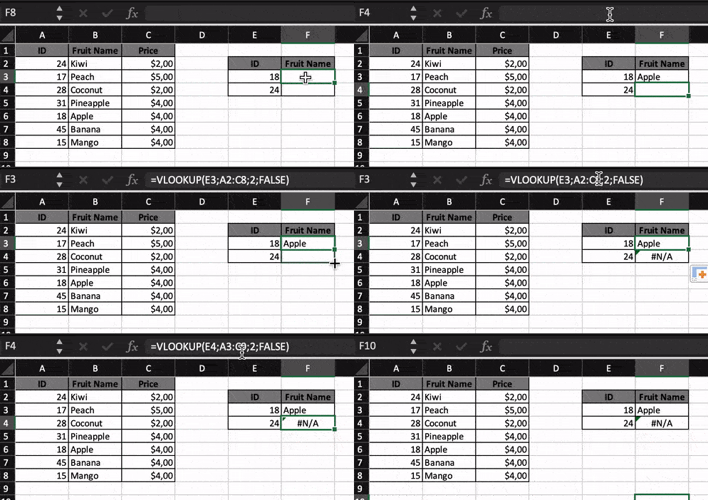
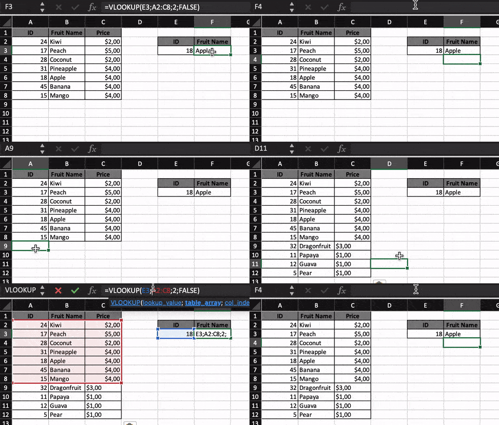
#1: Exact match in the VLOOKUP formula is not specified
Issue
On the following screenshot, we have a VLOOKUP formula, which returns an incorrect result. The correct vlookup result for ID 18 is Apple not Peach.
Solution
Enter FALSE as the last parameter if you are looking for an exact match. The correct VLOOKUP formula is
=VLOOKUP(E3,A2:C8,2,FALSE)
Explanation
The last parameter in the VLOOKUP function is Closest match (TRUE) or Exact match (FALSE). Most people are searching for a certain match such as for customer name, product name or employee name that need an exact match. FALSE should be entered for the last parameter in your VLOOKUP formula when you are looking for an exact value.
#2: The range in the VLOOKUP formula is not locked
Issue
When you drag your working Excel VLOOKUP formula down
=VLOOKUP(E3,A2:C8,2,FALSE)
it returns the #N/A error.
Solution
You need to lock the range in your VLOOKUP formula before dragging it or copying to other cells. To do this, type $ around the range as shown below:
Your VLOOKUP formula should look like this:
=VLOOKUP(E3,$A$2:$C$8,2,FALSE)
Now you can drag it without any errors expected.
Explanation
Once you dragged your VLOOKUP formula, the range in it changed, which caused the error.
#3: A new column has been inserted to the range
Issue
A new column was inserted and affected the range that was specified in your VLOOKUP formula.
=VLOOKUP(E3,A2:C8,2,FALSE)
Solution
To avoid this in the future, you need to make the column number dynamic using the MATCH function. This allows you to retrieve the matched position of a lookup value and column number. In this way, any new inserted columns won’t affect your VLOOKUP formula.
We updated our formula, so it looks like this.
=VLOOKUP(F3,A2:D8,MATCH(G2,A1:D1,0),FALSE)
G2– the value to match in lookup range.A1:D1– the lookup range.0– exact match type.
Let’s test the new lookup range by adding more columns as shown in the figure below:
The result does not change.
#4: Your table has gotten bigger
Issue
Your VLOOKUP formula was made for a specific limited range. You’ll have to update the formula manually every time when the range grows with new rows. Or not?
Solution
Not only can you set the column dynamic, but also the range, by giving it a name. This will help you ensure your VLOOKUP function always checks the whole table by following these steps:
- Select the range of cells you want to use for the lookup range. Click Home → Format as Table and choose Orange, Table Style Medium 3 (or any other style you desire).
- Specify your lookup range:
$A$1:$C$12. Check the box My table has headers then click OK as shown in the screenshot below:
- Update your lookup range in the VLOOKUP formula as follows:
Let’s test the new lookup range by adding one more row. Check your VLOOKUP by searching the new ID that you just added to the lookup range. The result returns the correct value as shown in figure below:
#5: Reverse VLOOKUP for those who do not have XLOOKUP in their version of Excel
Issue
The VLOOKUP formula cannot look up a value to the left, and your Excel does not have XLOOKUP.
Solution
You can vlookup to the left using the combination of the INDEX and MATCH functions:
- Suppose you want to look up the ID for Coconut from the table below:
- Type the following formula below in cell F3:
=INDEX(A2:A8,MATCH(E3,B2:B8,0))
INDEX– a function in Excel that returns the value from a certain location in a range.A2:A8– the range column where ID is stored is from A2-A8.MATCH– a function in Excel that used to locate the position of a lookup value in a table/column/row.E3– where ‘Coconut’ is located.B2:B8– the range column where Coconut is stored from B2:B8.0– an exact match of the return value.
- The result is:
Is there any difference between VLOOKUP in Excel and Google Sheets
Basically, VLOOKUP in Excel and Google Sheets has the same logic and the same syntax. So, if you migrate to Excel from Google Sheets, you won’t have any troubles. But of course, there are some differences. Check out our blog post about VLOOKUP in Google Sheets to find them. Good luck with looking up your data!
-
Technical Content Writer on Coupler.io who loves working with data, writing about it, and even producing videos about it. I’ve worked at startups and product companies, writing content for technical audiences of all sorts. You’ll often see me cycling🚴🏼♂️, backpacking around the world🌎, and playing heavy board games.
Back to Blog
Focus on your business
goals while we take care of your data!
Try Coupler.io
This Excel tutorial explains how to use the VLOOKUP function with syntax and examples.
Description
The VLOOKUP function performs a vertical lookup by searching for a value in the first column of a table and returning the value in the same row in the index_number position.
The VLOOKUP function is a built-in function in Excel that is categorized as a Lookup/Reference Function. It can be used as a worksheet function (WS) in Excel. As a worksheet function, the VLOOKUP function can be entered as part of a formula in a cell of a worksheet.
Subscribe
The VLOOKUP function is actually quite easy to use once you understand how it works! If you want to follow along with this tutorial, download the example spreadsheet.
Download Example
Syntax
The syntax for the VLOOKUP function in Microsoft Excel is:
VLOOKUP( value, table, index_number, [approximate_match] )
Parameters or Arguments
- value
- The value to search for in the first column of the table.
- table
- Two or more columns of data that is sorted in ascending order.
- index_number
- The column number in table from which the matching value must be returned. The first column is 1.
- approximate_match
- Optional. Enter FALSE to find an exact match. Enter TRUE to find an approximate match. If this parameter is omitted, TRUE is the default.
Returns
The VLOOKUP function returns any datatype such as a string, numeric, date, etc.
If you specify FALSE for the approximate_match parameter and no exact match is found, then the VLOOKUP function will return #N/A.
If you specify TRUE for the approximate_match parameter and no exact match is found, then the next smaller value is returned.
If index_number is less than 1, the VLOOKUP function will return #VALUE!.
If index_number is greater than the number of columns in table, the VLOOKUP function will return #REF!.
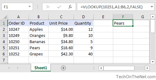
Example (as Worksheet Function)
Let’s explore how to use VLOOKUP as a worksheet function in Microsoft Excel.
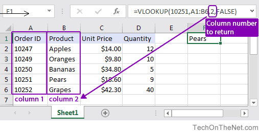
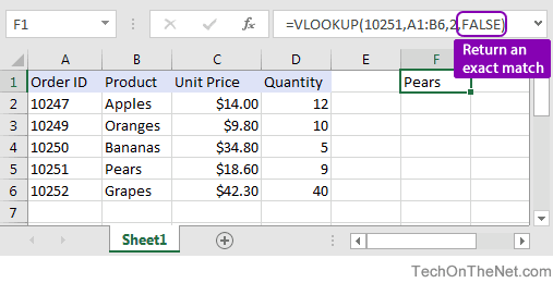
Based on the Excel spreadsheet above, the following VLOOKUP examples would return:
=VLOOKUP(10251, A1:B6, 2, FALSE)
Result: "Pears"   'Returns value in 2nd column

=VLOOKUP(10251, A1:C6, 3, FALSE)
Result: $18.60    'Returns value in 3rd column

=VLOOKUP(10251, A1:D6, 4, FALSE)
Result: 9         'Returns value in 4th column

=VLOOKUP(10248, A1:B6, 2, FALSE)
Result: #N/A      'Returns #N/A error (no exact match)

=VLOOKUP(10248, A1:B6, 2, TRUE)
Result: "Apples"  'Returns an approximate match
Now, let’s look at the example =VLOOKUP(10251, A1:B6, 2, FALSE) that returns a value of «Pears» and take a closer look why.
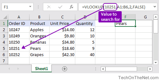
First Parameter
The first parameter in the VLOOKUP function is the value to search for in the table of data.
In this example, the first parameter is 10251. This is the value that the VLOOKUP will search for in the first column of the table of data. Because it is a numeric value, you can just enter the number. But if the search value was text, you would need to put it in double quotes, for example:
=VLOOKUP("10251", A1:B6, 2, FALSE)
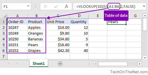
Second Parameter
The second parameter in the VLOOKUP function is the table or the source of data where the vertical lookup should be performed.
In this example, the second parameter is A1:B6 which gives us two columns to data to use in the vertical lookup — A1:A6 and B1:B6. The first column in the range (A1:A6) is used to search for the Order value of 10251. The second column in the range (B1:B6) contains the value to return which is the Product value.
Third Parameter
The third parameter is the position number in the table where the return data can be found. A value of 1 indicates the first column in the table. The second column is 2, and so on.
In this example, the third parameter is 2. This means that the second column in the table is where we will find the value to return. Since the table range is set to A1:B6, the return value will be in the second column somewhere in the range B1:B6.
Fourth Parameter
Finally and most importantly is the fourth or last parameter in the VLOOKUP. This parameter determines whether you are looking for an exact match or approximate match.
In this example, the fourth parameter is FALSE. A parameter of FALSE means that VLOOKUP is looking for an EXACT match for the value of 10251. A parameter of TRUE means that a «close» match will be returned. Since the VLOOKUP is able to find the value of 10251 in the range A1:A6, it returns the corresponding value from B1:B6 which is Pears.
Exact Match vs. Approximate Match
To find an exact match, use FALSE as the final parameter. To find an approximate match, use TRUE as the final parameter.
Let’s lookup a value that does not exist in our data to demonstrate the importance of this parameter!
Exact Match
Use FALSE to find an exact match:
=VLOOKUP(10248, A1:B6, 2, FALSE)
Result: #N/A
If no exact match is found, #N/A is returned.
Approximate Match
Use TRUE to find an approximate match:
=VLOOKUP(10248, A1:B6, 2, TRUE)
Result: "Apples"
If no match is found, it returns the next smaller value which in this case is «Apples».
VLOOKUP from Another Sheet
You can use the VLOOKUP to lookup a value when the table is on another sheet. Let’s modify our example above and assume that the table is in a different Sheet called Sheet2 in the range A1:B6.
We could rewrite our original example where we lookup the value 10251 as follows:
=VLOOKUP(10251, Sheet2!A1:B6, 2, FALSE)
By preceding the table range with the sheet name and an exclamation mark, we can update our VLOOKUP to reference a table on another sheet.
VLOOKUP from Another Sheet with Spaces in Sheet Name
Let’s throw in one more complication. What happens if your sheet name contains spaces? If there are spaces in the sheet name, you will need to change the formula further.
Let’s assume that the table is on a Sheet called «Test Sheet» in the range A1:B6, now we need to wrap the Sheet name in single quotes as follows:
=VLOOKUP(10251, 'Test Sheet'!A1:B6, 2, FALSE)
By placing the sheet name within single quotes, we can handle a sheet name with spaces in the VLOOKUP function.
VLOOKUP from Another Workbook
You can use the VLOOKUP to lookup a value in another workbook. For example, if you wanted to have the table portion of the VLOOKUP formula be from an external workbook, we could try the following formula:
=VLOOKUP(10251, 'C:[data.xlsx]Sheet1'!$A$1:$B$6, 2, FALSE)
This would look for the value 10251 in the file C:data.xlxs in Sheet 1 where the table data is found in the range $A$1:$B$6.
Why use Absolute Referencing?
Now it is important for us to cover one more mistake that is commonly made. When people use the VLOOKUP function, they commonly use relative referencing for the table range like we did in some of our examples above. This will return the right answer, but what happens when you copy the formula to another cell? The table range will be adjusted by Excel and change relative to where you paste the new formula. Let’s explain further…
So if you had the following formula in cell G1:
=VLOOKUP(10251, A1:B6, 2, FALSE)
And then you copied this formula from cell G1 to cell H2, it would modify the VLOOKUP formula to this:
=VLOOKUP(10251, B2:C7, 2, FALSE)
Since your table is found in the range A1:B6 and not B2:C7, your formula would return erroneous results in cell H2. To ensure that your range is not changed, try referencing your table range using absolute referencing as follows:
=VLOOKUP(10251, $A$1:$B$6, 2, FALSE)
Now if you copy this formula to another cell, your table range will remain $A$1:$B$6.
How to Handle #N/A Errors
Next, let’s look at how to handle instances where the VLOOKUP function does not find a match and returns the #N/A error. In most cases, you don’t want to see #N/A but would rather display a more user-friendly result.
For example, if you had the following formula:
=VLOOKUP(10248, $A$1:$B$6, 2, FALSE)
Instead of displaying #N/A error if you do not find a match, you could return the value «Not Found». To do this, you could modify your VLOOKUP formula as follows:
=IF(ISNA(VLOOKUP(10248, $A$1:$B$6, 2, FALSE)), "Not Found", VLOOKUP(10248, $A$1:$B$6, 2, FALSE))
OR
=IFERROR(VLOOKUP(10248, $A$1:$B$6, 2, FALSE), "Not Found")
OR
=IFNA(VLOOKUP(10248, $A$1:$B$6, 2, FALSE), "Not Found")
These formulas use the ISNA, IFERROR and IFNA functions to return «Not Found» if a match is not found by the VLOOKUP function.
This is a great way to spruce up your spreadsheet so that you don’t see traditional Excel errors.
Frequently Asked Questions
If you want to find out what others have asked about the VLOOKUP function, go to our Frequently Asked Questions.
Frequently Asked Questions
В табличном редакторе Microsoft Excel множество различных формул и функций. Они позволяют сэкономить время и избежать ошибок – достаточно правильно написать формулу и подставить нужные значения.
В этой статье мы рассмотрим функцию ВПР (или VLOOKUP, что означает «вертикальный просмотр»). Функция ВПР помогает работать с данными из двух таблиц и подтягивать значения из одной в другую. Использовать ее удобно, когда нужно посчитать выручку или прикинуть бюджет, если в одной таблице указан прайс-лист, а в другой количество проданного товара.
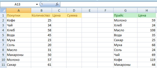
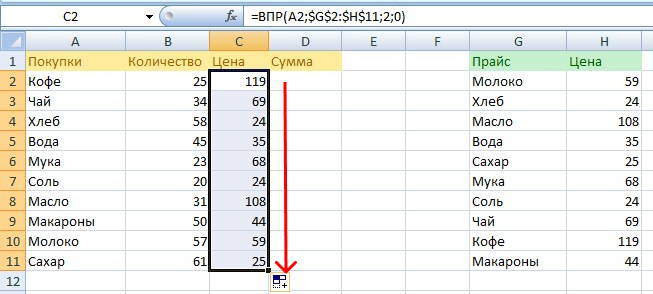
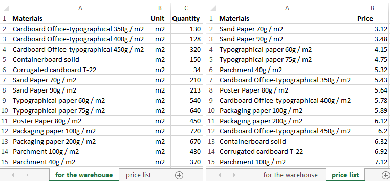
Допустим, есть таблица с количеством проданного товара и таблица с ценами на эти товары
Необходимо к каждому товару из таблицы слева добавить цену из прайса справа.
Как создать функцию ВПР в Excel
Необходимая последовательность значений в функции называется синтаксис. Обычно функция начинается с символа равенства «=», затем идет название функции и аргументы в скобках.
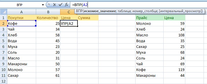
Записываем формулу в столбик цены (С2). Это можно сделать двумя способами:
-
Выделить ячейку и вписать функцию.
-
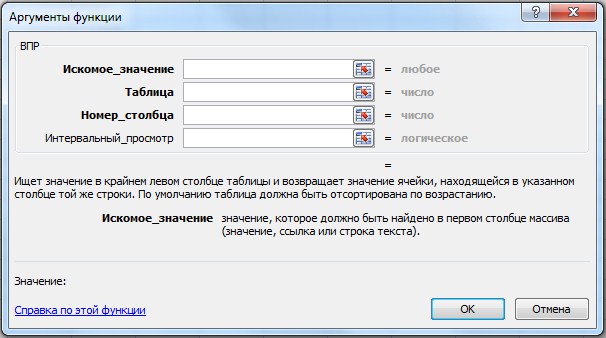
Выделить ячейку → нажать на Fx (Shift +F3) → выбрать категорию «Ссылки и массивы» → выбрать функцию ВПР → нажать «ОК».
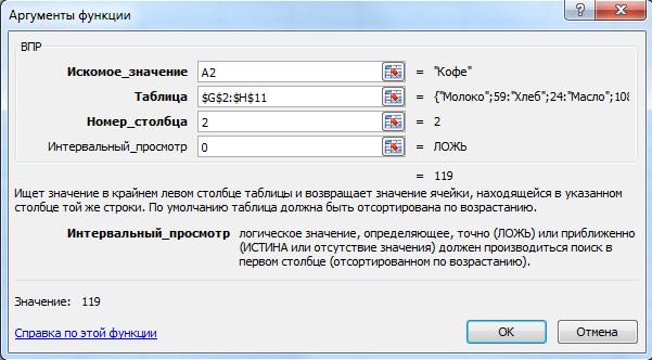
После этого открывается окно, где можно заполнить ячейки аргументов формулы.
Синтаксис функции ВПР выглядит так:
=ВПР(искомое значение;таблица;номер столбца;интервальный просмотр)
В нашем случае получится такая формула:
=ВПР(A2;$G$2:$H$11;2;0)
Аргументы функции ВПР
Сейчас разберемся что и куда писать.
Со знаком равенства «=» и названием «ВПР» все понятно. Поговорим об аргументах. Они записываются в скобках через точку с запятой или заполняются в ячейки в окне функции. Формула ВПР имеет 4 аргумента: искомое значение, таблица, номер столбца и интервальный просмотр.
Искомое значение – это название ячейки, из которой мы будем «подтягивать» данные. Формула ВПР ищет полное или частичное совпадение в другой таблице, из которой берет информацию.
В нашем случае выбираем ячейку «A2», в ней находится наименование товара. ВПР возьмет это название и будет искать аналогичную ячейку во второй таблице с прайсом.
=ВПР(A2;
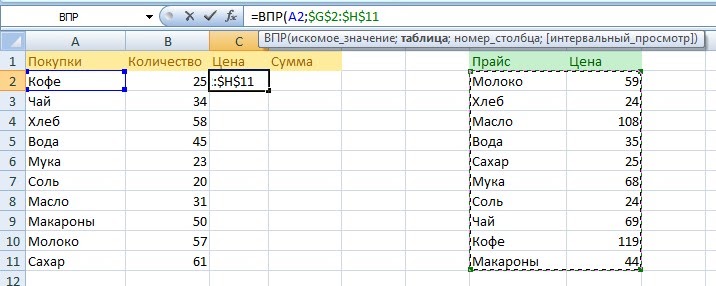
Таблица – это диапазон ячеек, из которых мы будем «подтягивать» данные для искомого значения. В этом аргументе используем абсолютные ссылки. Это значит, что в формуле таблица будет выглядеть как «$G$2:$H$11» вместо «G2:H11». Знаки «$» можно поставить вручную, а можно выделить «G2:H11» внутри формулы и нажать F4. Если этого не сделать, таблица не зафиксируется в формуле и изменится при копировании.
В нашем случае – это таблица с прайсом. Формула будет искать в ней совпадение с ячейкой, которую указали в первом аргументе формулы – A2 (Кофе). Нажимаем F4 и делаем ссылку абсолютной.
=ВПР(A2;$G$2:$H$11
Номер столбца – это столбец таблицы, из которой нужно взять данные. Именно из него мы будем «подтягивать» результат.
-
Формула сканирует таблицу по вертикали.
-
Находит в самом левом столбце совпадение с искомым значением.
-
Смотрит в столбец напротив, очередность которого мы указываем в этом аргументе.
-
Передает данные в ячейку с формулой.
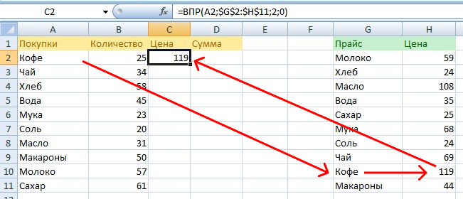
В нашем случае – это столбец с ценой продуктов в прайсе. Формула ищет искомое значение ячейки A2 (Кофе) в первом столбце прайса и «подтягивает» данные из второго столбца (потому что мы указали цифру 2) в ячейку с формулой.
=ВПР(A2;$G$2:$H$11;2
Интервальный просмотр – это параметр, который может принимать 2 значения: «истина» или «ложь». Истина обозначается в формуле цифрой 1 и означает приблизительное совпадение с искомым значением. Ложь обозначается цифрой 0 и подразумевает точное совпадение. Приблизительный поиск и критерий «истина» обычно используют при работе с числами, а точный и «ложь» – в работе с наименованиями.
В нашем случае искомое значение – это текстовое наименование. Поэтому используем точный поиск – ставим цифру 0 и закрываем скобку.
=ВПР(A2;$G$2:$H$11;2;0)
Комьюнити теперь в Телеграм
Подпишитесь и будьте в курсе последних IT-новостей
Подписаться
Автозаполнение
В конце протягиваем формулу вниз до конца, в результате чего происходит автозаполнение.
Чтобы функция ВПР правильно сработала во время автозаполнения, искомое значение должно быть относительной ссылкой, а таблица – абсолютной.
-
В нашем случае искомое значение – A2. Это относительная ссылка на ячейку, потому что в ней нет знаков «$». Благодаря этому ссылка на искомое значение меняется относительно каждой строчки, когда происходит автозаполнение в другие ячейки: A2 → A3 → … → A11. Это удобно, когда необходимо повторить формулу на несколько строк, ведь ее не приходится писать заново.
-
Таблица зафиксирована абсолютной ссылкой «$G$2:$H$11». Это означает, что ссылки на ячейки не изменятся во время автозаполнения. Таким образом, расчет каждый раз будет корректным и опираться на таблицу.
ВПР и приблизительный интервальный просмотр
В предыдущем примере мы «подтягивали» значения из таблицы, используя точный интервальный просмотр. Он подходит для работы с наименованиями. Теперь разберем ситуацию, когда может понадобиться приблизительный интервальный просмотр.
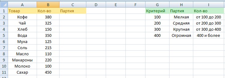
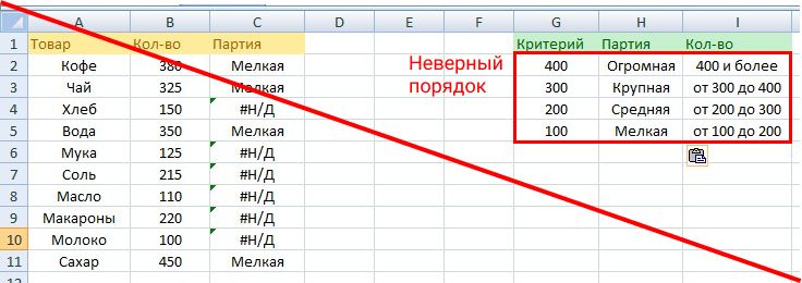
Задача. В магазин привезли товар. Необходимо присвоить каждому товару размер партии, опираясь на его количество.
Товары такие же, как и в первом примере, но задача изменилась: нужно привязать формулу не к наименованию, а к количеству
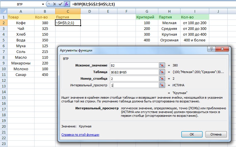
Решение. Заполняем формулу ВПР в ячейке «Партия», как было показано в предыдущем примере.
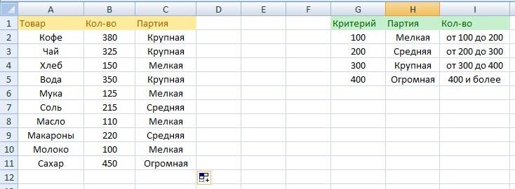
Разница в том, что теперь искомое значение – число, а интервальный просмотр – истина, что означает приблизительный поиск. Получается вот такой результат:
Что произошло? Аргумент «интервальный просмотр» имеет значение 1. Это значит, что формула ВПР ищет в таблице ближайшее меньшее искомое значение.
В нашем случае количество товара «Кофе» – 380. ВПР берет это число в виде искомого значения, после чего ищет ближайшее меньшее в соседней таблице – число 300. В конце функция «подтягивает» данные из столбца напротив («Крупная»). Если количество товара «Кофе» = 340 – это «Крупная партия». Важно, чтобы крайний левый столбец таблицы, которая указана в формуле, был отсортирован по возрастанию. В противном случае ВПР не сработает.
Значения и данные во второй таблице отсортированы по убыванию – ВПР не работает
Итоги
-
Функция ВПР означает вертикальный просмотр. Она просматривает крайний левый столбец таблицы сверху вниз.
-
Синтаксис функции: =ВПР(искомое значение;таблица;номер столбца;интервальный просмотр).
-
Функцию можно вписать вручную или в специальном окне (Shift + F3).
-
Искомое значение – относительная ссылка, а таблица – абсолютная.
-
Интервальный просмотр может искать точное или приблизительное совпадение с искомым значением.
-
Приблизительный поиск и критерий «истина» обычно используют при работе с числами, а точный и «ложь» – в работе с наименованиями.
-
Порядок работы с функцией подходит для Гугл-таблиц.
The Function VLOOKUP in Excel allows rearranging data from one table to the corresponding cells in another one.
It’s very handy and frequently used. As it’s a problematic thing to compare manually ranges with tens of thousands of names.
How to use The Function VLOOKUP in Excel
For example, the warehouse of the enterprise for the production of packaging received materials in a certain amount. The cost of materials is in the price list. This is a separate table.
It is necessary to find out the cost of materials received at the warehouse. To do this we should substitute the price of the second table in the first. And by ordinary multiplication we will find the title.
Algorithm:
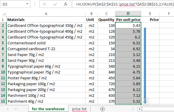
- Here is the first table (for the warehouse) in the required view. Add columns «Per unit price» and total «Price». Establish a currency format for the new cells.
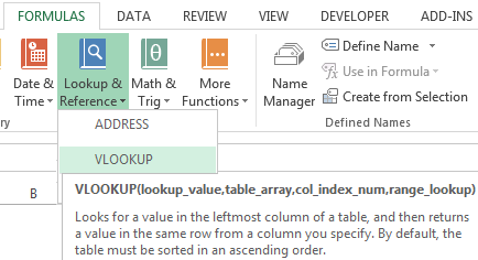
- Select the first cell in the «Price» column. In our example it’s D2. Call the «Insert Function» using the «FX» button (at the beginning of the formula bar) or by pressing the hot key combination SHIFT + F3. In the category «Lookup & Reference» we find the function =VLOOKUP(), and click OK. This function can be called up by clicking on the «FORMULAS» tab and choose from the drop-down list of «Lookup & Reference».
- A window with the function arguments will be opened. In the field «Lookup_value» — the first column of the range of data from the table with the number of received materials. These are the values that Excel should find in the second table.
- The next argument is «Table_array». This is our price list. Put the cursor in the field of argument than go to the list prices. Select the range with the names of materials and prices. Show what value the function should match.
- For Excel to refer directly to these data, it is necessary to fix the link. Select «Table_array» field value and press F4. $ Icon appears.
- In the argument «Col_index_num» put the number «2». Here are the data that you need to get in the first table. «Range_lookup» is FALSE. As we need specific, not approximate.
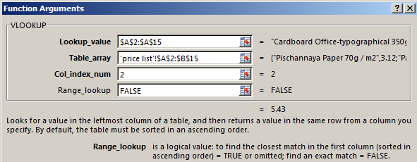
Click OK. And then copy the function of that column: we catch a mouse bottom right corner and drag down. We get the necessary result.
Now to find the cost of materials is not difficult: the number of * cost.
Function VLOOKUP linked the two tables. If you change the price, and then change the value of the materials received at the warehouse (now received). To avoid this, use the «Paste Special».
- Select the column with inserted prices.
- Use the right mouse button – «Copy».
- Still selected use the right mouse button – «Paste Special».
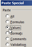
- Put a tick next to «Values». OK.
The formulas in the cells disappear. Only values remain.
A quick comparison of the two tables with the help of VLOOKUP
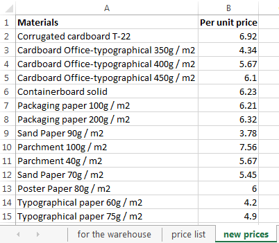
The function helps to compare the values in large tables. In case of the price has changed. We need to compare the old prices with the new prices.
- In the old price list do the column «NEW Price».
- Select the first cell and select the function VLOOKUP. The given examples (see. Above). For example:
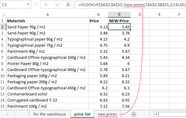
This means that you need to take the name of the material from the range A2: A15, look it up in the «new prices» in column A. Then take the data from the second column of the new price (Per unit price) and substitute them in cell C2 under «NEW Price».
The data presented in this way, can be compared. We can find the numeral and percentage difference.
The function VLOOKUP in Excel with multiple conditions
Until now, we have offered for the analysis of only one condition — the name of the material. In practice, it often requires several bands to compare and select the data value 2, 3 and other criteria.
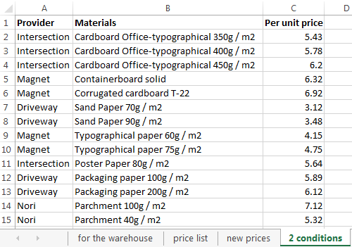
Table for example:
Guessing we need to find, what is the price of the corrugated cardboard of JSC «Magnet». It is necessary to set two conditions to search the name of the material and the vendor.
The matter is complicated by the fact that one supplier receives several names.
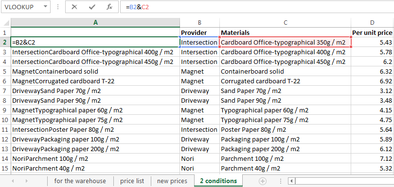
- Adding to the table the leftmost column (important!), combining the «Provider» and «Materials».
- We combine the required criteria the same way:
- Put the cursor in the right place H3 and set arguments for function:

Excel finds the right price.
Consider the formula in detail:
- What we are looking for – request the addition of a criterion F3&G3.
- Where to look for – range of data A2:D15.
- What data to take – column number 4 in the range A2:D15.
The Function VLOOKUP and drop-down list
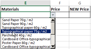
For example, some data is made in the form of a drop-down list. In our example it is «Materials». It is necessary to configure the function so that when choosing names appeared prices.
First do drop-down list:
- Go to sheet «price list» and create a table for requests in the range E1:G2.
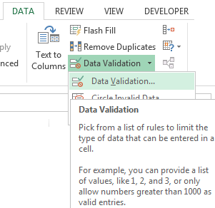
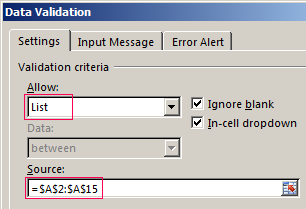
- Put the cursor in cell F3, where will be this list and go to the tab «DATA». «Data Validation» menu.
- Select the type of data – «List». Source is the range with the names of materials.
- When press the OK the dropdown list is formed.
Now you need to make the way when choosing a particular material in the column price corresponding figure appeared. Put the cursor in the F2 cell (which will have to appear the price).
- Open the window «Insert Function» and select VLOOKUP.
- The first argument is «Lookup_value» – the box with drop-down list. The table is a range of materials with names and prices. And column 2. Function has acquired the following form:
- In a cell G2, enter the formula (formula different column number 3):
- Press ENTER and enjoy the result.
Change the material — the price changes:
Download this example VLOOKUP in Excel
This is how the drop down list in Excel with the function of the VLOOKUP. Everything happens automatically within a few seconds. Everything works quickly and accurately. It is necessary to deal with this function.


