
Word vectors represent a significant leap forward in advancing our ability to analyze relationships across words, sentences, and documents. In doing so, they advance technology by providing machines with much more information about words than has previously been possible using traditional representations of words. It is word vectors that make technologies such as speech recognition and machine translation possible. There are many excellent explanations of word vectors, but in this one, I want to make the concept accessible to data and research people who aren’t very familiar with natural language processing (NLP).
What Are Word Vectors?
A word vector is an attempt to mathematically represent the meaning of a word. A computer goes through the text and calculates how often words show up next to each other. It is useful, first of all, to consider why word vectors are considered such a leap forward from traditional representations of words.
Traditional approaches to NLP, such as one-hot encoding and bag-of-words models (i.e. using dummy variables to represent the presence or absence of a word in an observation, i.e. a sentence), while useful for some machine learning (ML) tasks, do not capture information about a word’s meaning or context. This means that potential relationships, such as contextual closeness, are not captured across collections of words. For example, a one-hot encoding cannot capture simple relationships, such as determining that the words «dog» and «cat» both refer to animals that are often discussed in the context of household pets. Such encodings often provide sufficient baselines for simple NLP tasks (for example, email spam classifiers), but lack the sophistication for more complex tasks such as translation and speech recognition. In essence, traditional approaches to NLP such as one-hot encodings do not capture syntactic (structure) and semantic (meaning) relationships across collections of words and, therefore, represent language in a very naive way.
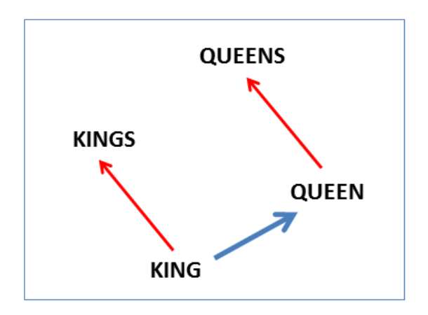
In contrast, word vectors represent words as multidimensional continuous floating point numbers where semantically similar words are mapped to proximate points in geometric space. In simpler terms, a word vector is a row of real-valued numbers (as opposed to dummy numbers) where each point captures a dimension of the word’s meaning and where semantically similar words have similar vectors. This means that words such as wheel and engine should have similar word vectors to the word car (because of the similarity of their meanings), whereas the word banana should be quite distant. Put differently, words that are used in a similar context will be mapped to a proximate vector space (we will get to how these word vectors are created below). The beauty of representing words as vectors is that they lend themselves to mathematical operators. For example, we can add and subtract vectors — the canonical example here is showing that by using word vectors we can determine that:
-
king — man + woman = queen
In other words, we can subtract one meaning from the word vector for king (i.e. maleness), add another meaning (femaleness), and show that this new word vector (king — man + woman) maps most closely to the word vector for queen.
The numbers in the word vector represent the word’s distributed weight across dimensions. In a simplified sense, each dimension represents a meaning and the word’s numerical weight on that dimension captures the closeness of its association with and to that meaning. Thus, the semantics of the word are embedded across the dimensions of the vector.
A Simplified Representation of Word Vectors
In the figure, we are imagining that each dimension captures a clearly defined meaning. For example, if you imagine that the first dimension represents the meaning or concept of «animal,» then each word’s weight on that dimension represents how closely it relates to that concept.
This is quite a large simplification of word vectors as the dimensions do not hold such clearly defined meanings, but it is a useful and intuitive way to wrap your head around the concept of word vector dimensions.
We create a list of words, apply spaCy’s parser, extract the vector for each word, stack them together, and then extract two-principal components for visualization purposes.
import numpy as np
import spacy
from sklearn.decomposition import PCA
nlp = spacy.load("en")
animals = "dog cat hamster lion tiger elephant cheetah monkey gorilla antelope rabbit mouse rat zoo home pet fluffy wild domesticated"
animal_tokens = nlp(animals)
animal_vectors = np.vstack([word.vector for word in animal_tokens if word.has_vector])
pca = PCA(n_components=2)
animal_vecs_transformed = pca.fit_transform(animal_vectors)
animal_vecs_transformed = np.c_[animals.split(), animal_vecs_transformed]
Here, we simply extract vectors for different animals and words that might be used to describe some of them. As mentioned in the beginning, word vectors are amazingly powerful because they allow us (and machines) to identify similarities across different words by representing them in a continuous vector space. You can see here how the vectors for animals like «lion,» «tiger,» «cheetah,» and «elephant» are very close together. This is likely because they are often discussed in similar contexts; for example, these animals are big, wild and, potentially dangerous — indeed, the descriptive word «wild» maps quite closely to this group of animals.
Similar words are mapped together in the vector space. Notice how close «cat» and «dog» are to «pet,» how clustered «elephant,» «lion,» and «tiger» are, and how descriptive words also cluster together.
What is also interesting here is how closely the words «wild,» «zoo,» and «domesticated» map to one another. It makes sense given that they are words that are frequently used to describe animals, but highlights the amazing power of word vectors!
Where Do Word Vectors Come From?
An excellent question at this point is, Where do these dimensions and weights come from?! There are two common ways through which word vectors are generated:
- Counts of word/context co-occurrences
- Predictions of context given word (skip-gram neural network models, i.e. word2vec)
Note: Below, I describe a high-level word2vec approach to generating word vectors, but a good overview of the count/co-occurence approach can be found here.
Both approaches to generating word vectors build on Firth’s (1957) distributional hypothesis which states:
«You shall know a word by the company it keeps.»
Put differently, words that share similar contexts tend to have similar meanings. The context of a word in a practical sense refers to its surrounding word(s) and word vectors are (typically) generated by predicting the probability of a context given a word. Put differently, the weights that comprise a word vector are learned by making predictions on the probability that other words are contextually close to a given word. This is akin to attempting to fill in the blanks around some given input word. For example, given the input sequence, «The fluffy dog barked as it chased a cat,» the two-window (two-words preceding and proceeding the focal word) context for the words «dog» and «barked» would look like:
I don’t wish to delve into the mathematical details how neural networks learn word embeddings too much, as people much more qualified to do so have explicated this already. In particular, these posts have been helpful to me when trying to understand how word vectors are learned:
- Deep Learning, NLP, and Representations
- The Amazing Power of Word Vectors
- Word2Vec Tutorial: The Skip-Gram Model
It is useful, however, to touch on the workings of the word2vec model given its popularity and usefulness. A word2vec model is simply a neural network with a single hidden layer that is designed to reconstruct the context of words by estimating the probability that a word is «close» to another word given as input.
The model is trained on word, context pairings for every word in the corpus, i.e.:
-
(DOG, THE)(DOG), FLUFFY(DOG, BARKED)(DOG, AS)
Note that this is technically a supervised learning process, but you do not need labeled data — the labels (the targets/dependent variables) are generated from the words that form the context of a focal word. Thus, using the window function the model learns the context in which words are used. In this simple example, the model will learn that «fluffy» and «barked» are used in the context (as defined by the window length) of the word «dog.»
One of the fascinating things about word vectors created by word2vec models is that they are the side effects of a predictive task, not its output. In other words, a word vector is not predicted, (it is context probabilities that are predicted), the word vector is a learned representation of the input that is used on the predictive task — i.e. predicting a word given a context. The word vector is the model’s attempt to learn a good numerical representation of the word in order to minimize the loss (error) of its predictions. As the model iterates, it adjusts its neurons’ weights in an attempt to minimize the error of its predictions and in doing so, it gradually refines its representation of the word. In doing so, the word’s «meaning» becomes embedded in the weight learned by each neuron in the hidden layer of the network.
A word2vec model, therefore, accepts as input a single word (represented as a one-hot encoding amongst all words in the corpus) and the model attempts to predict the probability that a randomly chosen word in the corpus is at a nearby position to the input word. This means that for every input word there are n output probabilities, where n is equal to the total size of the corpus. The magic here is that the training process includes only the word’s context, not all words in the corpus. This means in our simple example above, given the word «dog» as input, «barked» will have a higher probability estimate than «cat» because it is closer in context, i.e. it is learned in the training process. Put differently, the model attempts to predict the probability that other words in the corpus belong to the context of the input word. Therefore, given the sentence above («The fluffy dog barked as it chased a cat») as input a run of the model would look like this:
Note: This conceptual NN is a close friend of the diagram in Chris McCormick’s blog post linked to above.
The value of going through this process is to extract the weights that have been learned by the neurons of the model’s hidden layer. It is these weights that form the word vector, i.e. if you have a 300-neuron hidden layer, you will create a 300-dimension word vector for each word in the corpus. The output of this process, therefore, is a word-vector mapping of size n-input words * n-hidden layer neurons.
Next Up
Word vectors are an amazingly powerful concept and a technology that will enable significant breakthroughs in NLP applications and research. They also highlight the beauty of neural network deep learning and, particularly, the power of learned representations of input data in hidden layers. In my next post, I will be using word vectors in a convolutional neural network for a classification task. This will highlight word vectors in practice, as well as how to bring pre-trained word vectors into a Keras model.
Data structure
Machine learning
neural network
NLP
Dimension (data warehouse)
Concept (generic programming)
Word2vec
Task (computing)
ANIMAL (image processing)
Network
How do you define word vectors? In this post, I will introduce you to the concept of word vectors. We’ll go over different types of word embeddings, and more importantly, how word vectors function. We’ll then be able to see the impact of word vectors on SEO, which will lead us to understand how Schema.org markup for structured data can help you take advantage of word vectors in SEO.
Keep reading this post if you wish to learn more about these topics.
Let’s dive right in.
Word vectors (also called Word embeddings) are a type of word representation that allows words with similar meanings to have an equal representation.
In simple terms: A word vector is a vector representation of a particular word.
According to Wikipedia:
It is a technique used in natural language processing (NLP) for representing words for text analysis, typically as a real-valued vector that encodes the meaning of the word so that words that are close in vector space are likely to have similar meanings.
The following example will help us to understand this better:
Look at these similar sentences:
Have a good day. and Have a great day.
They barely have a different meaning. If we construct an exhaustive vocabulary (let’s call it V), it would have V = {Have, a, good, great, day} combining all words. We could encode the word as follows.
The vector representation of a word may be a one-hot encoded vector where 1 represents the position where the word exists and 0 represents the rest
Have = [1,0,0,0,0]
a=[0,1,0,0,0]
good=[0,0,1,0,0]
great=[0,0,0,1,0]
day=[0,0,0,0,1]
Suppose our vocabulary has only five words: King, Queen, Man, Woman, and Child. We could encode the words as:
King = [1,0,0,0,0]
Queen = [0,1,0,0,0]
Man = [0,0,1,00]
Woman = [0,0,0,1,0]
Child = [0,0,0,0,1]
Types of word Embedding (Word Vectors)
Word Embedding is one such technique in which vectors represent text. Here are some of the more popular types of word Embedding:
- Frequency-based Embedding
- Prediction based Embedding
We will not go deep into Frequency-based Embedding and Prediction-based Embedding here, but you may find the following guides helpful to understand both:
An Intuitive Understanding of Word Embeddings and Quick Introduction to Bag-of-Words (BOW) and TF-IDF for Creating Features from Text
A brief introduction to WORD2Vec
While Frequency-based Embedding has gained popularity, there is still a void in understanding the context of words and limited in their word representations.
Prediction-based Embedding (WORD2Vec) was created, patented, and introduced to the NLP community in 2013 by a team of researchers led by Tomas Mikolov at Google.
According to Wikipedia, the word2vec algorithm uses a neural network model to learn word associations from a large corpus of text (large and structured set of texts).
Once trained, such a model can detect synonymous words or suggest additional words for a partial sentence. For example, with Word2Vec, you can easily create such results: King – man + woman = Queen, which was considered an almost magical result.
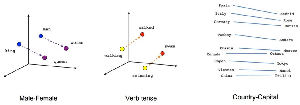 Image source: Tensorflow
- [king] – [man] + [woman] ~= [queen] (another way of thinking about this is that [king] – [queen] is encoding just the gendered part of [monarch])
- [walking] – [swimming] + [swam] ~= [walked] (or [swam] – [swimming] is encoding just the “past-tense-ness” of the verb)
- [madrid] – [spain] + [france] ~= [paris] (or [madrid] – [spain] ~= [paris] – [france] which is presumably roughly “capital”)
Source: Brainslab Digital
I know this is a little technical, but Stitch Fix put together a fantastic post about semantic relationships and word vectors.
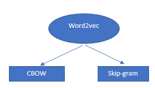
The Word2Vec algorithm is not a single algorithm but a combination of two techniques that uses a few AI methods to bridge human comprehension and machine comprehension. This technique is essential in solving many NLP problems.
These two techniques are:
- – CBOW (Continuous bag of words) or CBOW model
- – Skip-gram model.
Both are shallow neural networks that provide probabilities for words and have been proven helpful in tasks such as word comparison and word analogy.
How word vectors and word2vecs works
Word Vector is an AI model developed by Google, and it helps us solve very complex NLP tasks.
“Word Vector models have one central goal that you should know:
It is an algorithm that helps Google in detecting semantic relationships between words.”
Each word is encoded in a vector (as a number represented in multiple dimensions) to match vectors of words that appear in a similar context. Hence a dense vector is formed for the text.
These vector models map semantically similar phrases to nearby points based on equivalence, similarities, or relatedness of ideas and language
[Case Study] Driving growth in new markets with on-page SEO
When Springly began looking at expanding to the North American market, on-page SEO has been identified as one of the keys to a successful start in a new market. Find out how to go from 0 to success with technical SEO for your content strategy.
Word2Vec- How does it work?
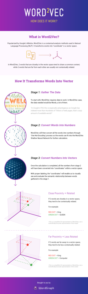
Image source: Seopressor
Pros and Cons of Word2Vec
We have seen that Word2vec is a very effective technique for generating distributional similarity. I have listed some of its other advantages here:
- There is no difficulty understanding Word2vec concepts. Word2Vec is not so complex that you aren’t aware of what is happening behind the scenes.
- Word2Vec’s architecture is very powerful and easy to use. Compared to other techniques, it is fast to train.
- Training is almost entirely automated here, so human-tagged data is no longer required.
- This technique works for both small and large datasets. As a result, it is an easy-to-scale model.
- If you know the concepts, you can easily replicate the entire concept and algorithm.
- It captures semantic similarity exceptionally well.
- Accurate and computationally efficient
- Since this approach is unsupervised, it is very time-saving in terms of effort.
Challenges of Word2Vec
The Word2vec concept is very efficient, but you may find a few points a bit challenging. Here are a few of the most common challenges.
- When developing a word2vec model for your dataset, debugging can be a major challenge, as the word2vec model is easy to develop but hard to debug.
- It does not deal with ambiguities. So, in the case of words with multiple meanings, Embedding will reflect the average of these meanings in vector space.
- Unable to handle unknown or OOV words: The biggest problem with word2vec is the inability to handle unknown or out-of-vocabulary (OOV) words.
Word Vectors: A Game-changer in Search Engine Optimization?
Many SEO experts believe Word Vector affects a website’s ranking in search engine results.
Over the past five years, Google has introduced two algorithm updates that put a clear focus on content quality and language comprehensiveness.
Let’s take a step back and talk about the updates:
Hummingbird
In 2013, Hummingbird gave search engines the capability of semantic analysis. By utilizing and incorporating semantics theory in their algorithms, they opened a new path to the world of search.
Google Hummingbird was the biggest change to the search engine since Caffeine in 2010. It gets its name from being “precise and fast”.
According to Search Engine Land, Hummingbird pays more attention to each word in a query, ensuring that the entire query is considered, rather than just particular words.
The main goal of Hummingbird was to deliver better results by understanding the context of the query rather than returning results for specific keywords.
“Google Hummingbird was released in September 2013.”
RankBrain
In 2015, Google announced RankBrain, a strategy that incorporated artificial intelligence (AI).
RankBrain is an algorithm that helps Google break down complex search queries into simpler ones. RankBrain converts search queries from “human” language into a language that Google can easily understand.
Google confirmed the use of RankBrain on 26 October 2015 in an article published by Bloomberg.
BERT
On 21 October 2019, BERT began rolling out in Google’s search system
BERT stands for Bidirectional Encoder Representations from Transformers, a neural network-based technique used by Google for pre-training in natural language processing (NLP).
In short, BERT helps computers understand language more like humans, and it is the biggest change in search since Google introduced RankBrain.
It is not a replacement for RankBrain, but rather an added method for understanding content and queries.
Google uses BERT in its ranking system as an addition. The RankBrain algorithm still exists for some queries and will continue to exist. But when Google feels that BERT can better understand a query, they will use that.
For more information on BERT, check out this post by Barry Schwartz, as well as Dawn Anderson’s in-depth dive.
Rank your site with Word Vectors
I’m assuming you already have created and published unique content, and even after polishing it over and over again, it does not improve your ranking or traffic.
Do you wonder why this is happening to you?
It might be because you didn’t include Word Vector: Google’s AI model.
- The first step is to Identify the Word Vectors of the top 10 SERP rankings for your niche.
- Know what keywords your competitors are using and what you might be overlooking.
By applying Word2Vec, which takes advantage of advanced Natural Language processing techniques and machine learning framework, you will be able to see everything in detail.
But these are possible if you know the machine learning and NLP techniques, but we can apply word vectors in the content using the following tool:
WordGraph, World’s First Word Vector Tool
This artificial intelligence tool is created with Neural Networks for Natural Language Processing and trained with Machine Learning.
Based on Artificial Intelligence, WordGraph analyzes your content and helps you improve its relevance to the Top 10 ranking websites.
It suggests keywords that are mathematically and contextually related to your main keyword.
Personally, I pair it up with BIQ, a powerful SEO tool that works well with WordGraph.
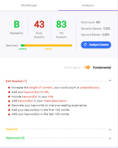
Add your content to the content intelligence tool built into Biq. It will show you a whole list of on-page SEO tips that you can add if you want to rank in the top position.
You can see how content intelligence works in this example. The lists will help you master on-page SEO and rank using actionable methods!
How to Supercharge Word Vectors: Using Structured Data Markup
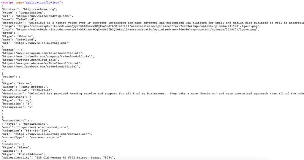
Schema markup, or structured data, is a type of code (written in JSON, Java-Script Object Notation) created using schema.org vocabulary that helps search engines to crawl, organize, and display your content.
How to add structured data
Structured data can be easily added to your website by adding an inline script in your html
An example below shows how to define your organization’s structured data in the simplest format possible.
To generate the Schema Markup, I use this Schema Markup Generator (JSON-LD).
Here is the live example of schema markup for https://www.telecloudvoip.com/. Check the source code and search for JSON.
After the schema markup code is created, use Google’s Rich Results Test to see if the page supports rich results.
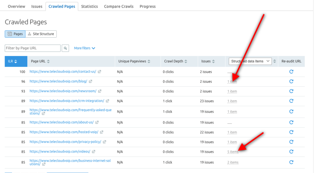
You can also use the Semrush Site Audit tool to explore Structured Data items for each URL and identify which pages are eligible for being in Rich Results.
Why is Structured Data Important for SEO?
Structured Data is important for SEO because it helps Google to understand what your website and pages are about, resulting in a more accurate ranking of your content.
Structured Data improves both the Search Bot’s experience as well as the user’s experience by improving the SERP (search engine result pages) with more information and accuracy.
To see the impact in Google search, go to Search Console and under Performance > Search Result > Search Appearance, you can view a breakdown of all the rich result types like “videos” and “FAQs” and see the organic impressions and clicks they drove for your content.
The following are some advantages of structured data:
- Structured data support semantic search
- It also supports your E‑A-T (expertise, authoritativeness, and trust)
- Having structured data can also increase conversion rates, since more people will see your listings, which increases the likelihood that they will buy from you.
- Using structured data the search engines are better able to understand your brand, your website, and your content.
- It will be easier for search engines to distinguish between contact pages, product descriptions, recipe pages, events pages, and customer reviews.
- With the help of structured data Google builds a better, more accurate knowledge graph and knowledge panel about your brand.
- These improvements can result in more organic impressions and organic clicks.
Structured data is currently used by Google to enhance search results. When people search for your web pages using keywords, structured data can help you get better results. Search engines will notice your content more if we add Schema markup.
You can implement schema markup on a number of different items. Listed below are a few areas where schema can be applied:
- Articles
- Blog Posts
- News Articles
- Events
- Products
- Videos
- Services
- Reviews
- Aggregate Ratings
- Restaurants
- Local businesses
Here’s a full list of the items you can mark up with schema.
Structured Data with Entity Embeddings
The term “entity” refers to a representation of any type of object, concept, or subject. An entity can be a person, movie, book, idea, place, company, or event.
While machines can’t really understand words, with entity embeddings, they are able to easily understand the relationship between king – queen = husband – wife
Entity embeddings perform better than one-hot encodings
The word vector algorithm is used by Google to discover semantic relationships between words, and when combined with structured data, we end up with a semantically enhanced web.
By using structured data, you are contributing to a more semantic web. This is an enhanced web where we describe the data in a machine-readable format.
Structured semantic data on your website helps search engines match your content with the right audience. The use of NLP, Machine Learning and Deep Learning helps reduce the gap between what people search for and what titles are available.
Final Thoughts
As you now understand the concept of word vectors and its importance, you can make your organic search strategy more effective and more efficient by utilizing word vectors, entity embeddings and structured semantic data.
In order to achieve the highest ranking, traffic, and conversions, you must use word vectors, entity embeddings and structured semantic data to demonstrate to Google that the content on your webpage is accurate, precise, and trustworthy.
Word vectors are representations of words
into numbers. Once words are in this form, it becomes straightforward for a
computer to understand them. Of course, you can’t just arbitrarily assign
numbers into words!
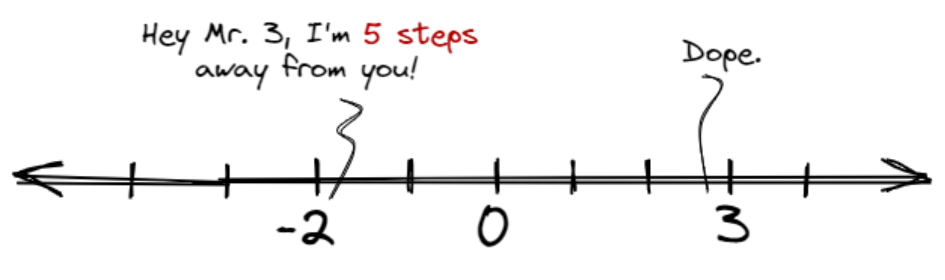
We need to satisfy two conditions: first, is that these numbers should have
some meaning, or semantics. Second, is that we should encode meaning
into a numerical representation. If we’re in the realm of numbers, a common way
to show meaning is to see how far one number is from another:
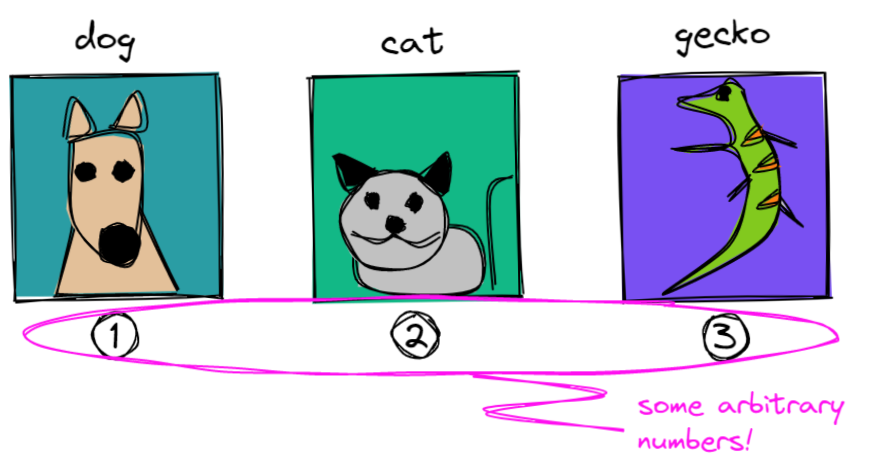
The hope is, words can also be represented as such. In the case of animals,
one trait, or feature, that we can encode is its leggedness. Let’s plot
our animals on a number line depending on the number of their legs:
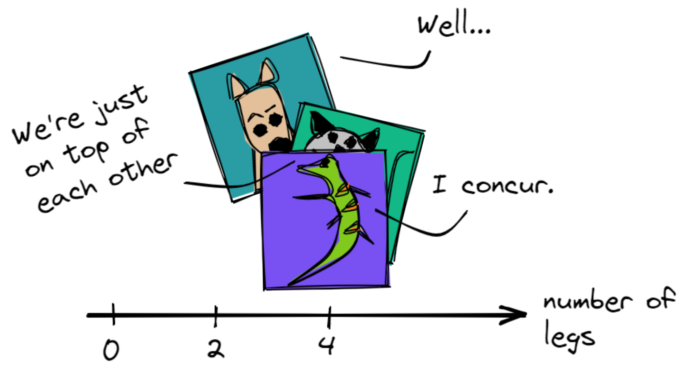
That’s not yet informative, all the animals were stacked on top of each other.
Perhaps we can add another feature, how about tameness? Let’s create another
axis and place our animals across them:
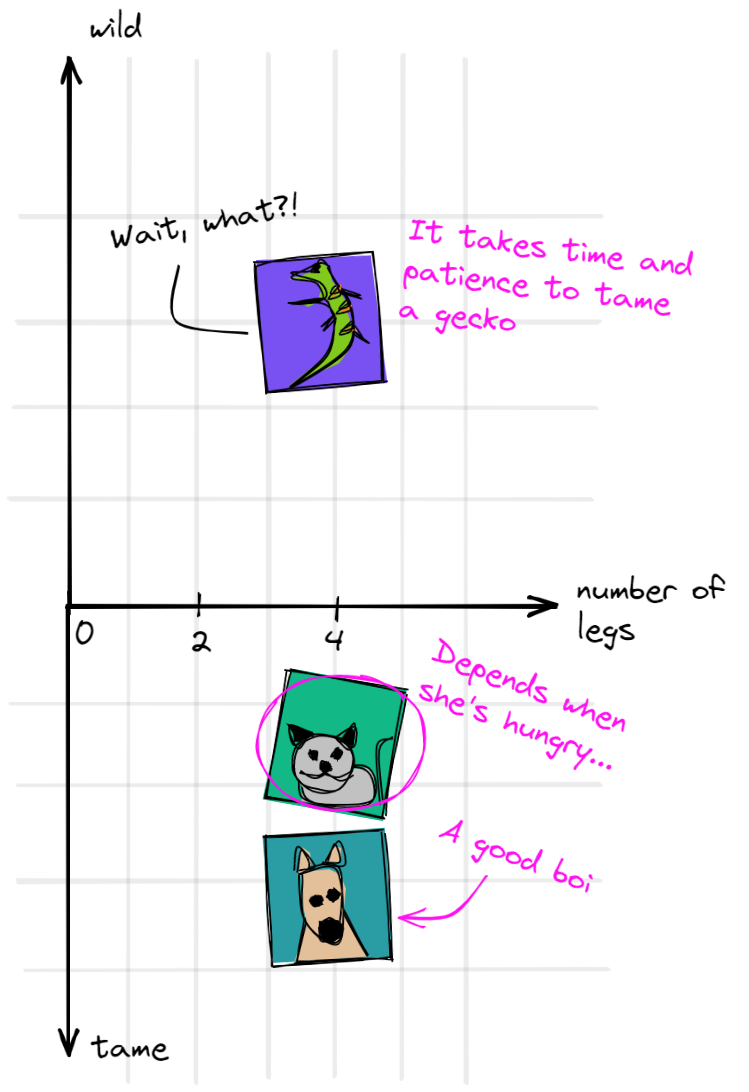
What we just did is that we came up with features and encoded them into our
vectors. As a result, we can now say that a dog is similar to a cat, entirely
different from a gecko, and so on.
But we don’t want to write all possible features one-by-one, we want to exploit
existing knowledge just for that. We also don’t want to encode them manually, we’d
rather write an algorithm to automate that for us.
This gives us to two ingredients in creating word vectors:
- An existing corpus of knowledge to get features automatically. Here, we
can use newspaper clippings, scraped data from the web, scientific
journals, and more! - An encoding mechanism to transfom that text into numbers. Instead of
writing them manually, we encode it algorithmically.
Contents
- On assigning numbers to words
- Word vectors from scratch
- Preliminary: the text corpus
- Clean the text
- Create word pairs
- Encode to one-hot vectors
- Train the model
- Post: model weights as vectors
- Looking back to what we can do now
We’ll use these two ingredients— the corpus and encoding
algorithm— to create word vectors from scratch. Some of these were
adapted from this
blogpost.
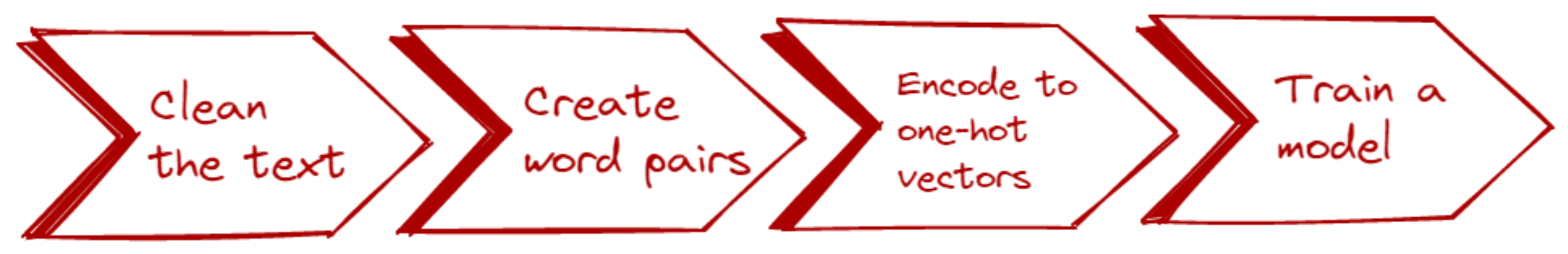
We’ll start from a small text corpus and end with a set of word vectors. The
process is as follows:
0. Preliminary: the text corpus 📚
Earlier, we manually encoded our knowledge into some mathematical format. When
we spoke of tameness, we assigned values to each of our animals and plotted them
into the graph. This method is great if you only deal with one or two features.
But when you want to capture the nuance and meaning ascribed to those words,
it’s not enough.
In practice, we extract knowledge from other sources: books, the Internet, Reddit
comments, Wikipedia, and more.
In practice, we’d want to extract knowledge from other sources—books,
the Internet, Reddit comments, Wikipedia…you name it! In NLP, we call
this collection of texts as the corpus.1 We won’t be scraping any text for
now. Instead, we’ll come up with our own:
sentences = [
    "A dog is an example of a canine",
    "A cat is an example of a feline",
    "A gecko can be a pet.",
    "A cat is a warm-blooded feline.",
    "A gecko is a cold-blooded reptile.",
    "A dog is a warm-blooded mammal.",
    "A gecko is an example of a reptile.",
    "A mammal is warm-blooded.",
    "A reptile is cold-blooded.",
    "A cat is a mammal.",
]
What you see above are factual statements about animals. Think of them as a
sample of sentences you’ll typically find in any corpus. In reality, ten
sentences aren’t enough to generate a good model, you’d want a larger corpus
for that. For example, the GloVe word
embeddings used Wikipedia, news
text, and the Internet (CommonCrawl) as its source.
It has hundreds of gigabytes of data, a million times more than the ten
sentences we have.
1. Clean the text 🧹
We clean the texts by removing stopwords and punctuations. In NLP, stopwords
are low-signal words that are uninformative and frequent.2 A few examples
include articles (a, an, the), some adverbs (actually, really), and a
few pronouns (he, me, it).
Most libraries like spaCy, nltk,
and gensim provide their own list of
stopwords. For us however, we’ll stick to writing our own:
STOP_WORDS = [
    "the",
    "a",
    "an",
    "and",
    "is",
    "are",
    "in",
    "be",
    "can",
    "I",
    "have",
    "of",
    "example",
    "so",
    "both",
]
We also write our own blacklist of punctuations:
PUNCTUATIONS = r"""!()-[]{};:'",<>./?@#$%^&*_~"""
We can now write our text cleaning function, clean_text. This function first
removes the punctuation by scanning each character and checking if it belongs
to our list. Then, it removes a stop word by scanning each word in the text.
A sample implementation is seen below:
from typing import List

def clean_text(
    text: str,
    punctuations: str = PUNCTUATIONS,
    stop_words: List = STOP_WORDS,
) -> List[str]:

    # Simple whitespace tokenization
    tokens = text.split()

    # Remove punctuations for each token
    tokens_no_puncts = []
    for token in tokens:
        for char in token.lower():
            if char in punctuations:
                token = token.replace(char, "")
        tokens_no_puncts.append(token)

    # Remove stopwords
    final_tokens = []
    for token in token_no_puncts:
        if token not in stop_words:
            final_tokens.append(token)

    return final_tokens
There’s one step that we haven’t talked about— tokenization. You can
see it subtly happening when we invoked text.split(). The goal of
tokenization is to segment our text into known boundaries. The easiest way to
achieve that is to split our sentence based on the whitespace, just like what
we did.
text = "A cat is a mammal."
print(clean_text(text))  # ["A", "cat", "is", "a", "mammal"]
Note that whitespace tokenization is not foolproof. This method won’t work
on languages that aren’t dependent on spaces (e.g., Chinese, Japanese,
Korean) or languages with different morphological rules (e.g., Arabic,
Indonesian). In fact, informal English also has a lot of special cases that
whitespace tokenization cannot solve (e.g. “Gimme” -> “Give me”).
# Cases where whitespace tokenization won't work
jp_text = "私の専門がコンピュタア工学 です"
kr_text = "비빔밥먹었어?"
In practice, you’d want to use more robust tokenizers for your language. For
example, spaCy offers a Tokenizer API that
can be customized to any language. spaCy uses its own tokenization
algorithm that
performs way better than our naive whitespace splitter.
If we run our clean_text function to all our sentences and obtain all unique
words, we’ll come up with a vocabulary:
# Clean each sentences first. We'll get a list of lists inside the
# all_text variable.
all_text = [clean_text(sentence) for sentence in sentences]

# We "flatten" our list and use the built-in set() function to get
# all unique elements of the list.
unique_words = set([word for text in all_text for word in text])
print(unique_words)  # ['canine', 'cat', 'coldblooded', ...]
From our small corpus, we obtained a measly vocabulary of size 10. On the
other hand, the CommonCrawl dataset has 42 billion tokens of web data…well,
we can’t be choosers, so let’s move on!
2. Create word pairs 🐾
As John Rupert Firth, a famous linguist, once said: “You shall know a word by
the company it keeps.”3 In this step, we create pairs consisting of each word
in our vocabulary and its context (“the company it keeps”). We call the former
as the center word and the latter as the context word.
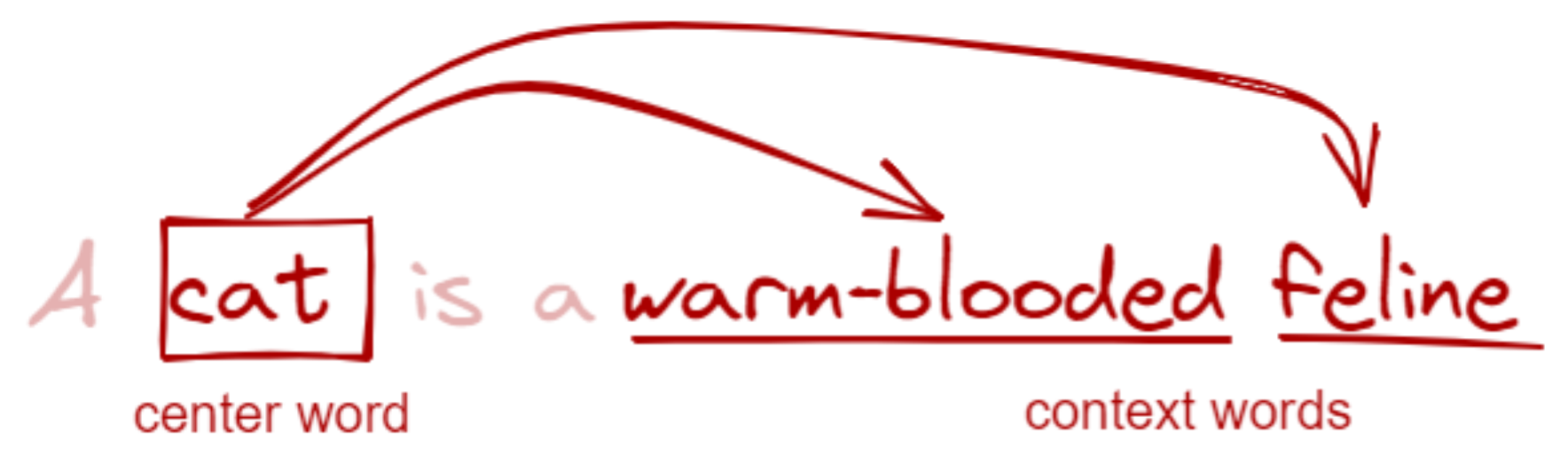
Figure: Demonstration of center and context words. Note that we skip
“a” and “is” because they’re stopwords. The clean_text function should’ve
removed them at this point.
You shall know a word by the company it keeps — John Rupert Firth
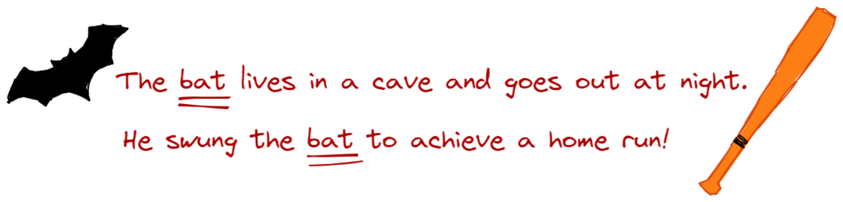
Context is important to understand meaning. Take the word bat for
example. We don’t know what it means in isolation, but in a sentence, its
meaning becomes crystal clear:
We can stretch this further: do you know the meaning of the words frumious,
Jabberwock, and Jubjub? Well, we can only guess. But in the context of
other words (in this case a poem), we can infer their meaning:
Beware the Jabberwock, my son!
The jaws that bite, the claws that catch!
Beware the Jubjub bird, and shun
The frumious Bandersnatch!
By looking at the context of each word, we now know that Jabberwock is a noun
and can be something dangerous because of the word ‘beware.’ It also has ‘jaws’
and ‘claws’ that bite and catch. Frumious, on the hand, is an adjective that
describes a Bandersnatch. Lastly, Jubjub could be a type of bird that one
should be beware of. Well…truth is, these words were just made up! I lifted
them from Lewis Carroll’s poem,
“Jabberwocky”, in
the novel Through the
Looking-Glass.
Awesome, huh?
We can also control the neighbors of a word through its window size. A size
of 1 means that a center word only sees adjacent words as its neighbor. Too
high a window and your context becomes less informative, too low and you fail
to capture all of its nuance.
Too high a window and your context becomes less informative, too low and you
fail to capture all of its nuance.
Now, we write a function to get word pairs from a sentence:
def create_word_pairs(
    text: List[str],
    window: int = 2
) -> List[Tuple[str, str]]:
    word_pairs = []
    for idx, word in enumerate(text):
        for w in range(window):
            if idx + 1 + w < len(text):
                pair = tuple([word] + [text[idx + 1 + w]])
                word_pairs.append(pair)
            if idx - w - 1 >= 0:
                pair = tuple([word] + [text[idx - w - 1]])
                word_pairs.append(pair)
    return word_pairs
Note that at this stage, we’ve already cleaned and tokenized our sentences.
We now pass a string of tokens and obtain a list of pairs.
text = "A cat is a warm-blooded feline."
cleaned_tokens = clean_text(text)  # ["cat", "warm-blooded", "feline"]

# Get word pairs
create_word_pairs(cleaned_tokens)
From here we obtain six pairs:
[('cat', 'warmblooded'),
 ('cat', 'feline'),
 ('warmblooded', 'feline'),
 ('warmblooded', 'cat'),
 ('feline', 'warmblooded'),
 ('feline', 'cat')]
We do this step for each text in our corpus. In the end, we obtain a large list
of pairs containing every word in our vocabulary and their corresponding
neighbor. The larger the corpus, the larger the expressivity of our word pairs.
In a way, having these pairs allows us to see which words tend to stick
together. Later on, we will train a model that can understand this affinity,
i.e., given a word (X), what’s the probability that a word (Y) will show
up? In the next section, we’ll jumpstart this stage by preparing our dataset.
3. Encode to one-hot vectors 🖥️
After obtaining word pairs, the next step is to convert them into some numerical
format. We won’t be overthinking this too much, so we’ll treat those numbers
similar to how we treat words— as discrete symbols. We accomplish this
with one-hot encoding.
In one-hot encoding, we prepare a table where each word in our vocabulary is
represented by a column. Our word columns don’t have to be in a specific order,
although I prefer sorting them alphabetically. To encode a word, we simply write
1 in the column where it is located and write 0 elsewhere:
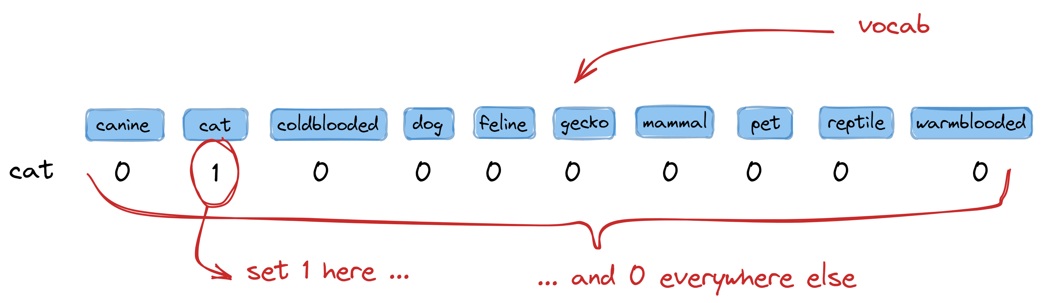
So for our corpus with a vocabulary size of 10, we create a table with ten columns.
To encode the word cat, we write 1 in the second column (where cat is located) and 0
elsewhere. This gives us the encoding:
>>> one_hot_encode("cat")  # I will show its implementation later!
[0, 1, 0, 0, 0, 0, 0, 0, 0, 0]
One advantage of one-hot encoding is that it allows us to interpret the encoded
vector as a probability distribution over our vocabulary. For example, if I have
a center word cat, we can then check how likely other words in our vocab will
appear as a context word:
# Note: not actual values. A highly-contrived example
# Numbers are just provided for illustration
>>> {v: l for v, l in vocab, get_likelihood("cat"))}
{
 "canine": 0.01,
 "cat": 0.27,
 "coldblooded": 0.01,
 "dog": 0.06,
 "feline": 0.22,
 "gecko": 0.04,
 "mammal": 0.11,
 "pet": 0.07,
 "reptile": 0.02,
 "warmblooded": 0.19,
}
One-hot encoding allows us to interpret the encoded vector as a
probability distribution over our vocabulary.
This also means that if we have the following word pair ("cat", "feline"),
their encoding can be interpreted as: “the word feline is likely to appear
given that the word cat is present.” It is consistent as long as we think of
zeroes and ones as probabilities:
>>> one_hot_encode("cat")
[0, 1, 0, 0, 0, 0, 0, 0, 0, 0]
>>> one_hot_encode("feline")
[0, 0, 0, 0, 1, 0, 0, 0, 0, 0]
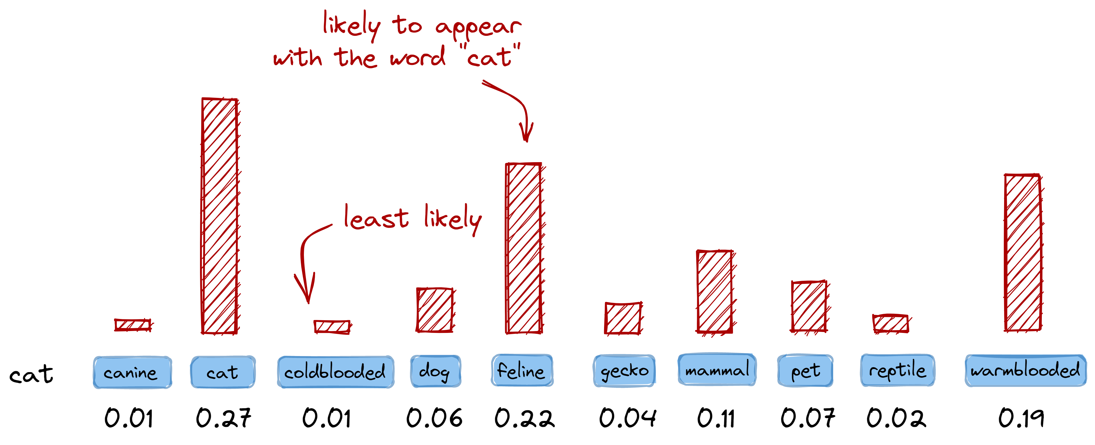
Figure: Vectors can also be interpreted as a probability distribution
over the vocabulary. This means that in one-hot encoding, a value of 1 may also
mean a highly-probable event.
(Note: this is a highly-contrived example)
One advantage of one-hot encoding is that it allows us to interpret the
encoded vector as a probability distribution over our vocabulary.
Now, let’s write a function to create one-hot encoded vectors from all our word
pairs and vocabulary. The vocabulary will guide us on the placement and length
of the one-hot vector. Lastly, instead of taking a single word, we’ll take a list
of word pairs to make things easier later on:
from typing import List, Tuple

def one_hot_encode(
    pairs: List[Tuple[str, str]],
    vocab: List[str]
) -> Tuple[List, List]:

    # We'll sort the vocabulary first.
    # It's not required, but it makes bookkeeping easier
    n_words = len(sorted(vocab))

    ctr_vectors = []  # center word placeholder
    ctx_vectors = []  # context word placeholder

    for pair in pairs:

        # Get center and context words
        ctr, ctx= pair
        ctr_idx = vocab.index(ctr)
        ctx_idx = vocab.index(ctx)

        # One-hot encode center words
        ctr_vector = [0] * n_words
        ctr_vector[ctr_idx] = 1
        ctr_vectors.append(ctr_vector)

        # One-hot encode context words
        ctx_vector = [0] * n_words
        ctx_vector[ctx_idx] = 1
        ctx_vectors.append(ctx_vector)

    return ctr_vectors, ctx_vectors
Now if we pass all our word pairs and vocabulary, we’ll get their corresponding
one-hot encoded center and context vectors:
sample_word_pairs = [("cat", "feline"), ("dog", "warm-blooded")]
vocab = ["canine", "cat", "cold-blooded", ...]

center_vectors, context_vectors = one_hot_encoded(sample_word_pairs, vocab)
print(center_vectors)
# gives:
# [[0, 1, 0, 0, 0, 0, 0, 0, 0, 0],
#  [0, 0, 0, 1, 0, 0, 0, 0, 0, 0]]
# for "cat" and "dog", our center words
print(context_vectors)
# gives:
# [[0, 0, 0, 0, 1, 0, 0, 0, 0, 0],
#  [0, 0, 0, 0, 0, 0, 0, 0, 0, 1]]
# for "feline" and "warm-blooded", our context words
In the next section, we will be using these two sets of vectors to train a
neural network model. The center vectors will act as our inputs, whereas the
context vectors will act as our labels.
4. Train a model 🤖
Because we now have a collection of center words with their corresponding context
words, it’s now possible to build a model that asks: “what is the likelihood
that a context word (y) appears given a center word (X)?” or simply,
(P(yvert x ; theta)).
To illustrate this idea: if the words warm-blooded, canine, and animal often appear
alongside the word dog, then that means we can infer something informative
about dogs. We just need to know how likely these words will come up, and that
will be the role of our model.
To train a model, we will use the center words as our input, and the context
words as our labels. We will build a neural network of size 10-2-10 with a
softmax layer in its output:
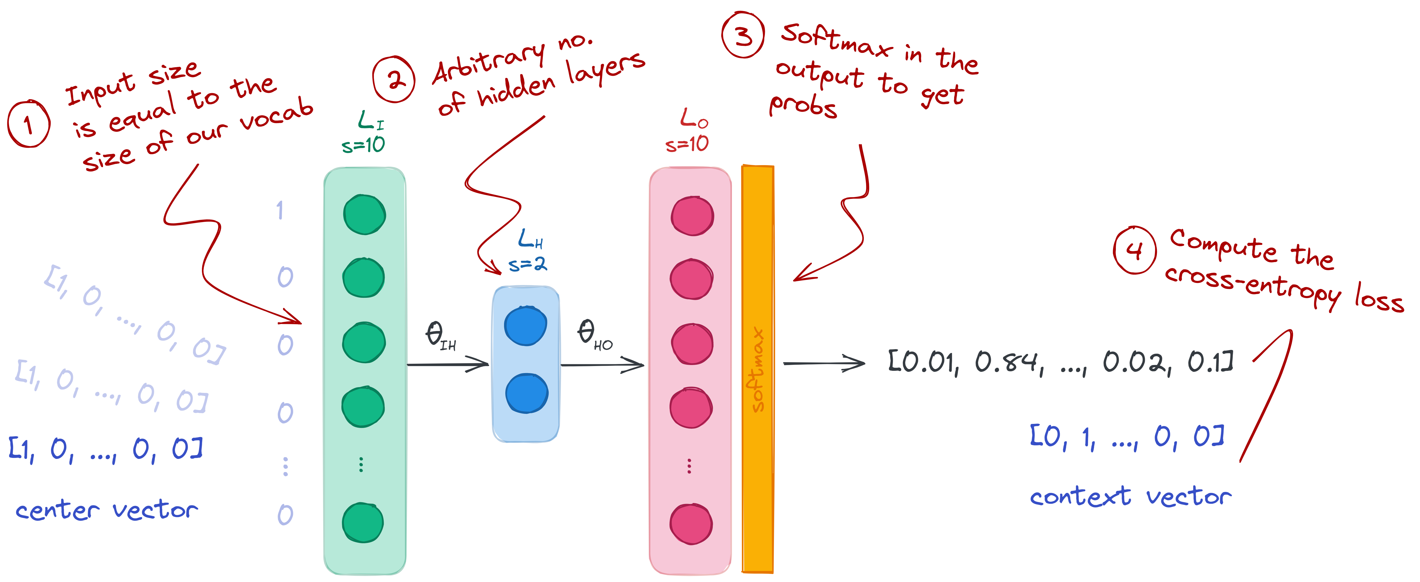
- Input layer (size 10): we set our input layer to the size of our vocabulary.
We don’t need to add an activation layer, so we just leave it as it is. - Hidden layer (size 2): this can be any arbitrary size, but I set it to 2 so that
I can plot the weights in a graph. It’s also possible to set a higher number, and perform
Principal Component Analysis (PCA) later on. - Output layer (size 10 with softmax): we set the number of nodes to 10 so
that we can compare it with the context vectors. The softmax activation is
important so that we can treat the output as probabilities and use cross-entropy
loss. To learn more about softmax, check my post on the negative
log-likelihood.
Now, let’s construct our neural network. We’ll use the following third-party
modules:
import torch
import torch.optim as optim
from torch import nn
We build our network based on the size of our center and context vectors.
For the hidden layer, we set an arbitrary size of 2.
# Prepare layer sizes
input_dim = len(center_vectors[0])
hidden_dim = 2
output_dim = len(context_vectors[0])

# Build the model
model = nn.Sequential(
    nn.Linear(input_dim, hidden_dim),
    nn.Linear(hidden_dim, output_dim),
)
Next we prepare our loss function and optimizer. We will use cross-entropy loss
to compute the difference between the model’s output and the context vector. In
Pytorch, softmax is already included when using the
torch.nn.CrossEntropyLoss
class, so there’s no need to add it in our model definition:
# In Pytorch, Softmax is already added when using CrossEntropyLoss
loss_fn = torch.nn.CrossEntropyLoss()
optimizer = optim.Adam(model.parameters(), lr=1e-4)
We also convert our vectors into Pytorch’s
FloatTensor data type. At this
stage, I’ll also call the center and context vectors as X and y
respectively, just to be consistent with common machine learning naming schemes:
X = torch.FloatTensor(center_vectors)
y = torch.FloatTensor(context_vector)
Lastly, we write our training loop. Because we’re using a deep learning
framework, we don’t have to write the backpropagation step by hand. Instead, we
simply call the backward()
method
from the loss function:
for t in range(int(1e3)):
    # Compute forward pass and print loss
    y_pred = model(X)
    loss = loss_fn(y_pred, torch.argmax(y, dim=1))
    # Zero the gradients before running the backward pass
    optimizer.zero_grad()
    # Backpropagation
    loss.backward()
    # Update weights using gradient descent
    optimizer.step()
After training the model, we can now access its weights. We’ll
obtain, in particular, the weights between the input and hidden layers:
name, weights = list(model.named_parameters())[0]
w = weights.data.tolist()
These weights are, in fact, our word vectors— congratulations!
They are of the same size as our hidden layer. I’ve set their dimension to 2 so
that we can plot the vectors right away into a graph. In the next section,
we’ll show what this graph looks like to get a deeper look into the behaviour of
our word vectors.
5. Post: on word vectors 🧮
After training our model, we took the weights between the input and hidden
layers to obtain our word embeddings. We specifically chose these weights
because they act as a lookup table for translating our one-hot encoded vectors
into a more suitable dimension.
The intermediary weight matrix (weights between the input and hidden layers)
acts as a lookup table that translates one-hot encoded vectors into a different
dimension.
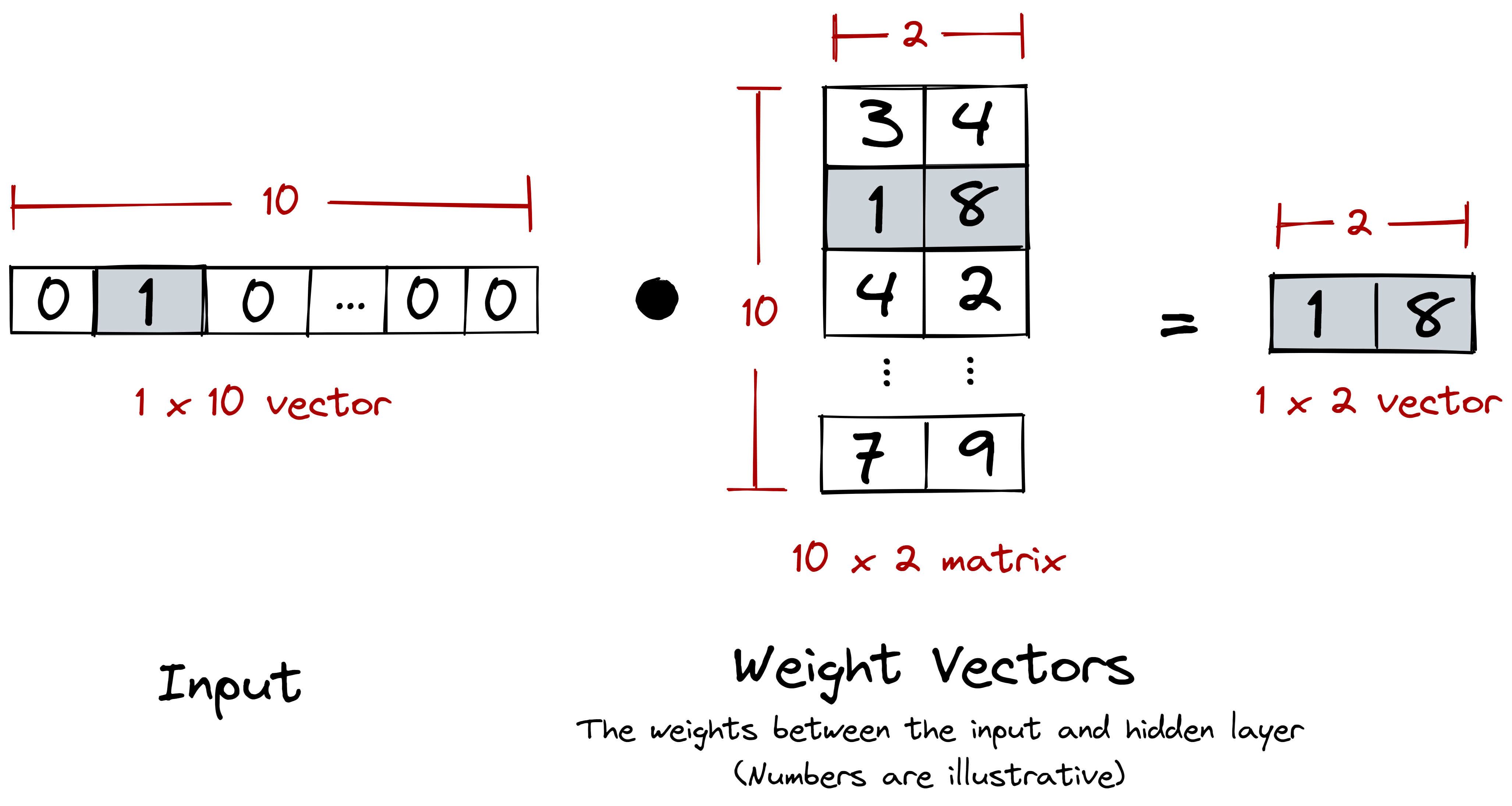
Figure: Our weight matrix, coupled with the one-hot encoded input, acts as a lookup table.
And this is definitely what we want. One-hot encoded vectors are sparse and
orthogonal: there’s really nothing that informative between [0 0 ... 1 0]
and [1 0 ... 0 0]. Instead, we want a dense vector where we can draw
meaningful semantic relations from. Our weight matrix performs this
transformation for us.
By having these dense and continuous relationships, we can even represent them into
a graph!
Notice how semantically related words are nearer to each other. For example, the
words gecko, reptile, and cold-blooded were clustered together. The same
goes for cat, dog, and warm-blooded. Even more so, these clusters of
“lizards” and “mammals” are further far apart!
We didn’t encode these relationships, it was all due to how the model
interpreted the words from our corpus. Sure, we wrote these sentences ourselves,
but in practice we just have to scrape them from somewhere.
Conclusion
In this blogpost, we looked into the idea of generating our own word vectors
from scratch. We achieved this by combining (1) a text corpus and (2) an
encoding mechanism. The word vectors we generated are crude, but we learned a
few things on how they came about. Truth is, what we just did is similar to the
original skip-gram implementation of Word2Vec
(Mikolov, et al, 2013): given a text corpus, we generate word pairs and train a
neural network across them.
In production, it is more ideal to use ready-made word embeddings—they are
more robust and generalizable. Of course, real-world NLP still requires
finetuning, but using these
vectors should already give you a headstart.
Lastly, I hope that this exercise made us more aware of how a text corpus can be
a source of bias: a corpus made up of Reddit comments will produce an entirely
different model compared to a corpus lifted from an encyclopedia. We can use
this for better or for worse: we can train “domain-specific” language models to
min/max our task,
or release models in the wild that are inherently biased. Real-world NLP isn’t
as easy as figuring out cats and dogs.
Footnotes
For today’s post, I’ve drawn material not just from one paper, but from five! The subject matter is ‘word2vec’ – the work of Mikolov et al. at Google on efficient vector representations of words (and what you can do with them). The papers are:
- Efficient Estimation of Word Representations in Vector Space – Mikolov et al. 2013
- Distributed Representations of Words and Phrases and their Compositionality – Mikolov et al. 2013
- Linguistic Regularities in Continuous Space Word Representations – Mikolov et al. 2013
- word2vec Parameter Learning Explained – Rong 2014
- word2vec Explained: Deriving Mikolov et al’s Negative Sampling Word-Embedding Method – Goldberg and Levy 2014
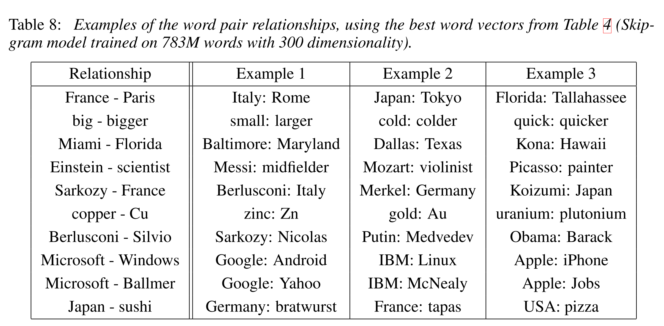
From the first of these papers (‘Efficient estimation…’) we get a description of the Continuous Bag-of-Words and Continuous Skip-gram models for learning word vectors (we’ll talk about what a word vector is in a moment…). From the second paper we get more illustrations of the power of word vectors, some additional information on optimisations for the skip-gram model (hierarchical softmax and negative sampling), and a discussion of applying word vectors to phrases. The third paper (‘Linguistic Regularities…’) describes vector-oriented reasoning based on word vectors and introduces the famous “King – Man + Woman = Queen” example. The last two papers give a more detailed explanation of some of the very concisely expressed ideas in the Milokov papers.
Check out the word2vec implementation on Google Code.
What is a word vector?
At one level, it’s simply a vector of weights. In a simple 1-of-N (or ‘one-hot’) encoding every element in the vector is associated with a word in the vocabulary. The encoding of a given word is simply the vector in which the corresponding element is set to one, and all other elements are zero.
Suppose our vocabulary has only five words: King, Queen, Man, Woman, and Child. We could encode the word ‘Queen’ as:
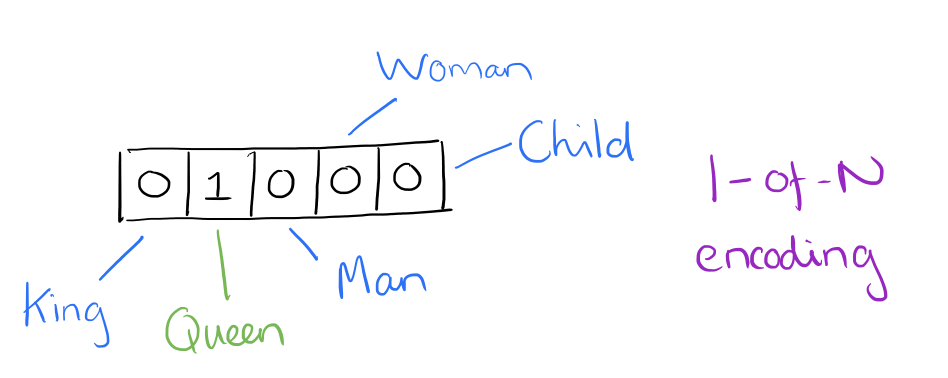
Using such an encoding, there’s no meaningful comparison we can make between word vectors other than equality testing.
In word2vec, a distributed representation of a word is used. Take a vector with several hundred dimensions (say 1000). Each word is representated by a distribution of weights across those elements. So instead of a one-to-one mapping between an element in the vector and a word, the representation of a word is spread across all of the elements in the vector, and each element in the vector contributes to the definition of many words.
If I label the dimensions in a hypothetical word vector (there are no such pre-assigned labels in the algorithm of course), it might look a bit like this:
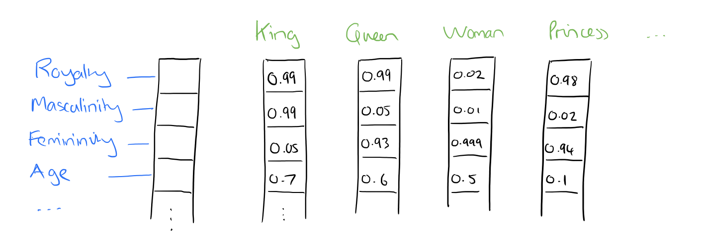
Such a vector comes to represent in some abstract way the ‘meaning’ of a word. And as we’ll see next, simply by examining a large corpus it’s possible to learn word vectors that are able to capture the relationships between words in a surprisingly expressive way. We can also use the vectors as inputs to a neural network.
Reasoning with word vectors
We find that the learned word representations in fact capture meaningful syntactic and semantic regularities in a very simple way. Specifically, the regularities are observed as constant vector offsets between pairs of words sharing a particular relationship. For example, if we denote the vector for word i as xi, and focus on the singular/plural relation, we observe that xapple – xapples ≈ xcar – xcars, xfamily – xfamilies ≈ xcar – xcars, and so on. Perhaps more surprisingly, we find that this is also the case for a variety of semantic relations, as measured by the SemEval 2012 task of measuring relation similarity.
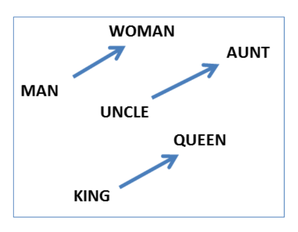
The vectors are very good at answering analogy questions of the form a is to b as c is to ?. For example, man is to woman as uncle is to ? (aunt) using a simple vector offset method based on cosine distance.
For example, here are vector offsets for three word pairs illustrating the gender relation:
And here we see the singular plural relation:
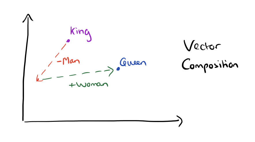
This kind of vector composition also lets us answer “King – Man + Woman = ?” question and arrive at the result “Queen” ! All of which is truly remarkable when you think that all of this knowledge simply comes from looking at lots of word in context (as we’ll see soon) with no other information provided about their semantics.
Somewhat surprisingly, it was found that similarity of word representations goes beyond simple syntatic regularities. Using a word offset technique where simple algebraic operations are performed on the word vectors, it was shown for example that vector(“King”) – vector(“Man”) + vector(“Woman”) results in a vector that is closest to the vector representation of the word Queen.
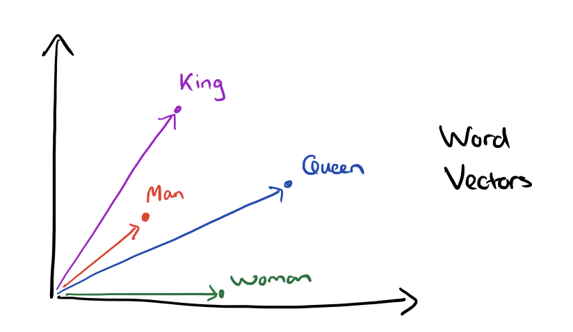
Vectors for King, Man, Queen, & Woman:
The result of the vector composition King – Man + Woman = ?
Here are some more results achieved using the same technique:
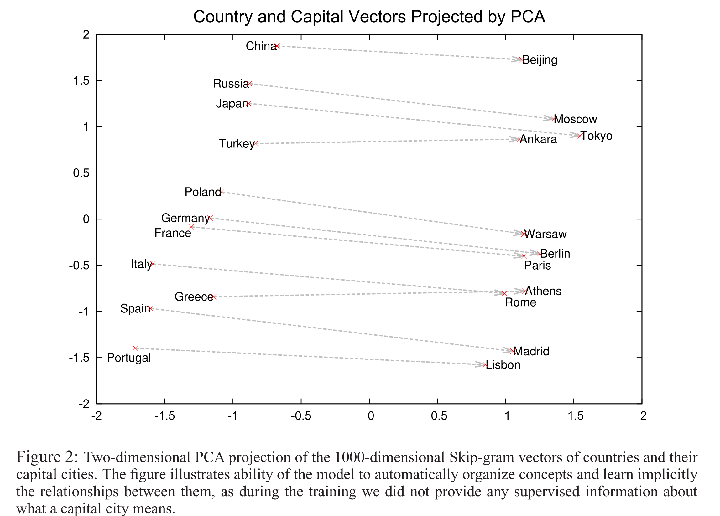
Here’s what the country-capital city relationship looks like in a 2-dimensional PCA projection:
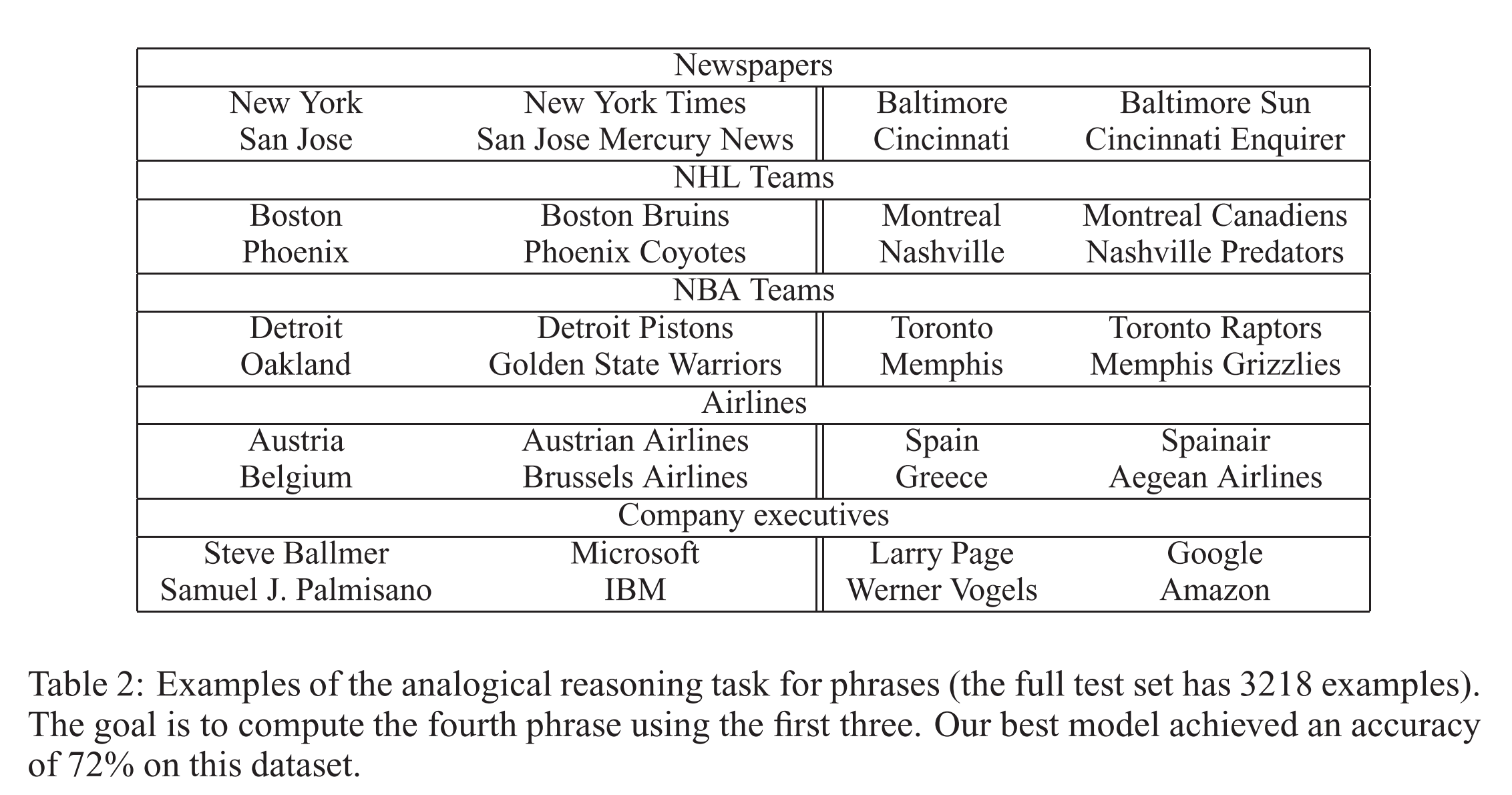
Here are some more examples of the ‘a is to b as c is to ?’ style questions answered by word vectors:
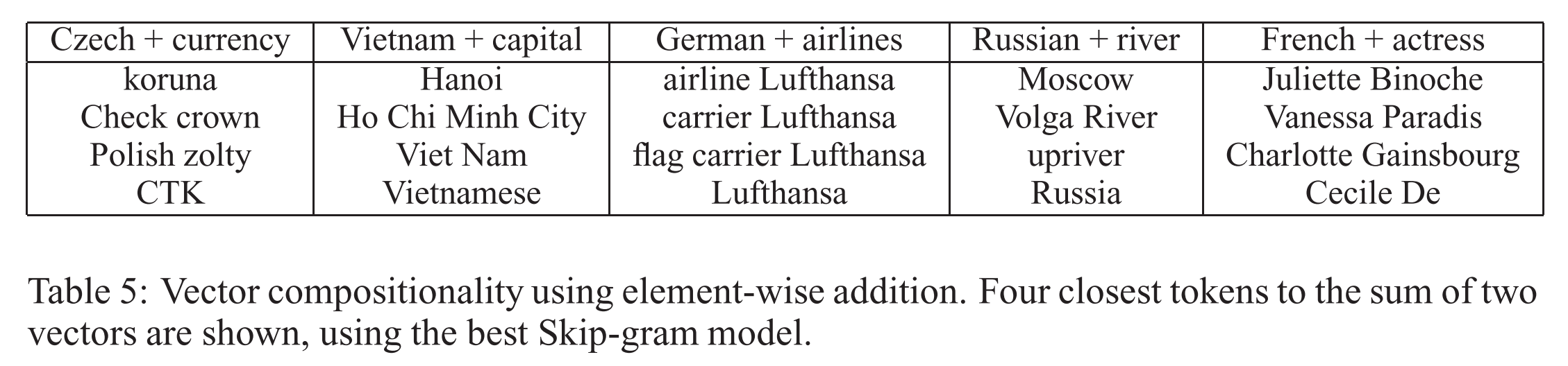
We can also use element-wise addition of vector elements to ask questions such as ‘German + airlines’ and by looking at the closest tokens to the composite vector come up with impressive answers:
Word vectors with such semantic relationships could be used to improve many existing NLP applications, such as machine translation, information retrieval and question answering systems, and may enable other future applications yet to be invented.
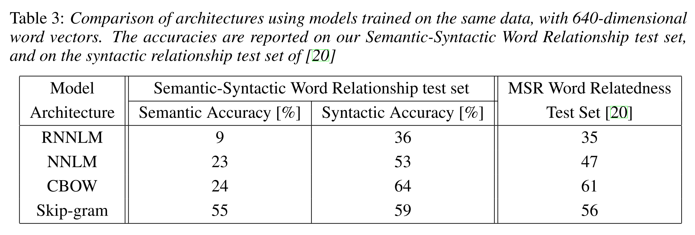
The Semantic-Syntatic word relationship tests for understanding of a wide variety of relationships as shown below. Using 640-dimensional word vectors, a skip-gram trained model achieved 55% semantic accuracy and 59% syntatic accuracy.
Learning word vectors
Mikolov et al. weren’t the first to use continuous vector representations of words, but they did show how to reduce the computational complexity of learning such representations – making it practical to learn high dimensional word vectors on a large amount of data. For example, “We have used a Google News corpus for training the word vectors. This corpus contains about 6B tokens. We have restricted the vocabulary size to the 1 million most frequent words…”
The complexity in neural network language models (feedforward or recurrent) comes from the non-linear hidden layer(s).
While this is what makes neural networks so attractive, we decided to explore simpler models that might not be able to represent the data as precisely as neural networks, but can posssible be trained on much more data efficiently.
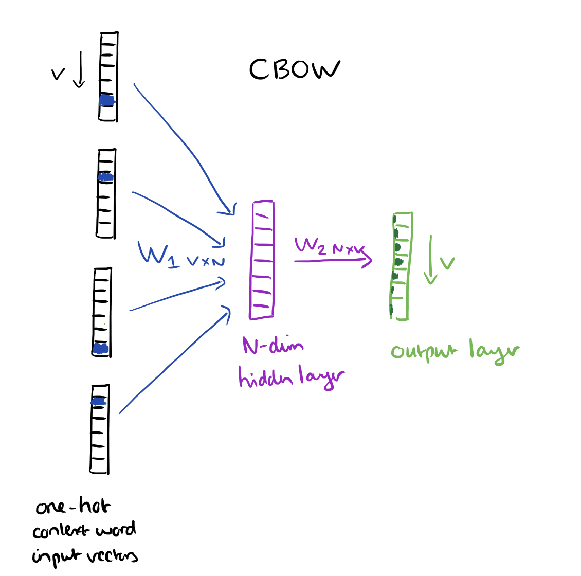
Two new architectures are proposed: a Continuous Bag-of-Words model, and a Continuous Skip-gram model. Let’s look at the continuous bag-of-words (CBOW) model first.
Consider a piece of prose such as “The recently introduced continuous Skip-gram model is an efficient method for learning high-quality distributed vector representations that capture a large number of precises syntatic and semantic word relationships.” Imagine a sliding window over the text, that includes the central word currently in focus, together with the four words and precede it, and the four words that follow it:
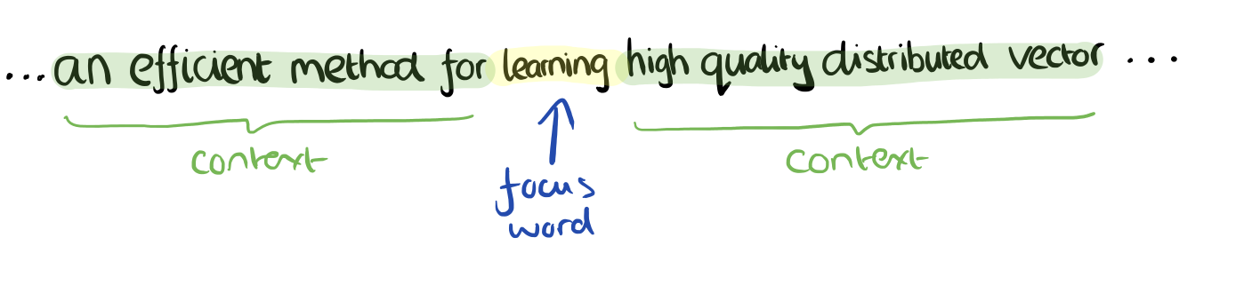
The context words form the input layer. Each word is encoded in one-hot form, so if the vocabulary size is V these will be V-dimensional vectors with just one of the elements set to one, and the rest all zeros. There is a single hidden layer and an output layer.
The training objective is to maximize the conditional probability of observing the actual output word (the focus word) given the input context words, with regard to the weights. In our example, given the input (“an”, “efficient”, “method”, “for”, “high”, “quality”, “distributed”, “vector”) we want to maximize the probability of getting “learning” as the output.
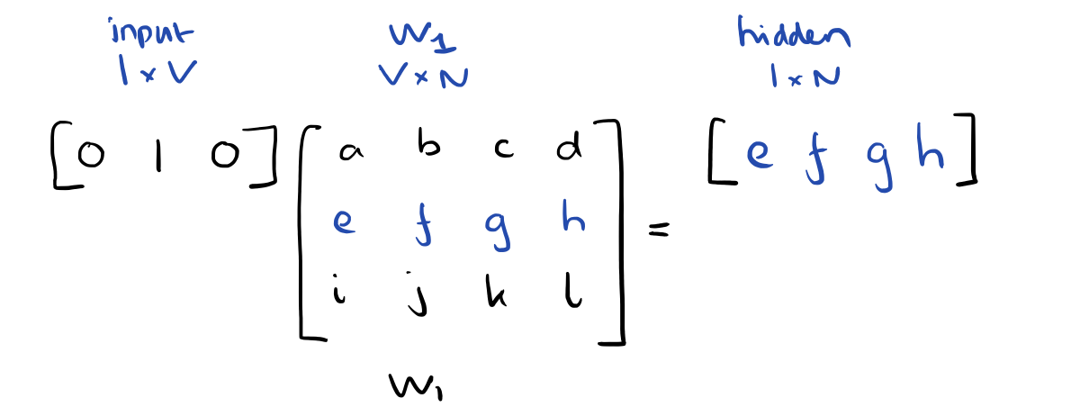
Since our input vectors are one-hot, multiplying an input vector by the weight matrix W1 amounts to simply selecting a row from W1.
Given C input word vectors, the activation function for the hidden layer h amounts to simply summing the corresponding ‘hot’ rows in W1, and dividing by C to take their average.
This implies that the link (activation) function of the hidden layer units is simply linear (i.e., directly passing its weighted sum of inputs to the next layer).
From the hidden layer to the output layer, the second weight matrix W2 can be used to compute a score for each word in the vocabulary, and softmax can be used to obtain the posterior distribution of words.
The skip-gram model is the opposite of the CBOW model. It is constructed with the focus word as the single input vector, and the target context words are now at the output layer:
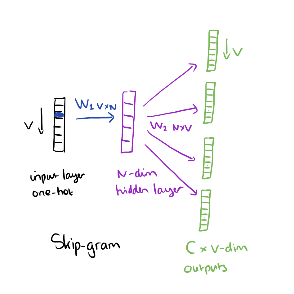
The activation function for the hidden layer simply amounts to copying the corresponding row from the weights matrix W1 (linear) as we saw before. At the output layer, we now output C multinomial distributions instead of just one. The training objective is to mimimize the summed prediction error across all context words in the output layer. In our example, the input would be “learning”, and we hope to see (“an”, “efficient”, “method”, “for”, “high”, “quality”, “distributed”, “vector”) at the output layer.
Optimisations
Having to update every output word vector for every word in a training instance is very expensive….
To solve this problem, an intuition is to limit the number of output vectors that must be updated per training instance. One elegant approach to achieving this is hierarchical softmax; another approach is through sampling.
Hierarchical softmax uses a binary tree to represent all words in the vocabulary. The words themselves are leaves in the tree. For each leaf, there exists a unique path from the root to the leaf, and this path is used to estimate the probability of the word represented by the leaf. “We define this probability as the probability of a random walk starting from the root ending at the leaf in question.”
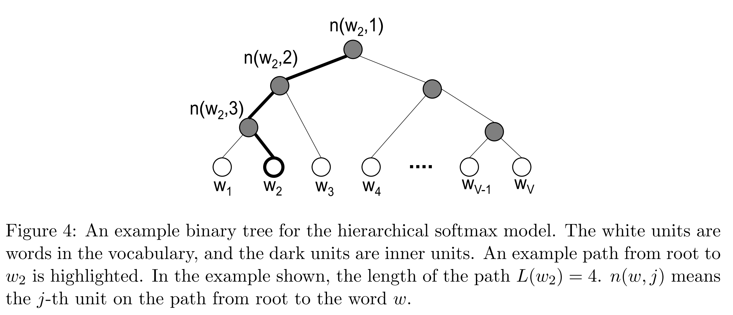
The main advantage is that instead of evaluating V output nodes in the neural network to obtain the probability distribution, it is needed to evaluate only about log2(V) words… In our work we use a binary Huffman tree, as it assigns short codes to the frequent words which results in fast training.
Negative Sampling is simply the idea that we only update a sample of output words per iteration. The target output word should be kept in the sample and gets updated, and we add to this a few (non-target) words as negative samples. “A probabilistic distribution is needed for the sampling process, and it can be arbitrarily chosen… One can determine a good distribution empirically.”
Mikolov et al. also use a simple subsampling approach to counter the imbalance between rare and frequent words in the training set (for example, “in”, “the”, and “a” provide less information value than rare words). Each word in the training set is discarded with probability P(wi) where
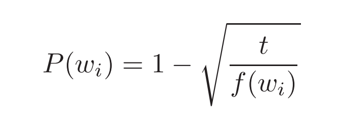
f(wi) is the frequency of word wi and t is a chosen threshold, typically around 10-5.
In this post we will look at representing text documents with word vectors, which are vectors of numbers that represent the meaning of a word.
Then we will write a custom Scikit-learn transformer class for the word vector features — similar to TfidfVectorizer or CountVectorizer — which can be plugged into a pipeline.
What are word vectors?
Word vectors, or word embeddings, are vectors of numbers that provide information about the meaning of a word, as well as its context.
You can get the semantic similarity of two words by comparing their word vectors.
Even if you’re not familiar with word vectors, you may have heard of a couple of popular algorithms for obtaining vectors for various words.
- GloVe
- word2vec
There are pre-trained models that you can download to access word vectors, and if you are using Spacy, GloVe vectors are made available in the larger models.
Accessing word vectors in Spacy
With Spacy you can easily get vectors of words, as well as sentences.
I’m assuming at least some familiarity with Spacy in this post.
Note that a small Spacy model — ending in sm, such as en_core_web_sm, will not have built-in vectors, so you will need a larger model to use them.
python -m spacy download en_core_web_lg
Vectors are made available in Spacy Token, Doc and Span objects.
import spacy

nlp = spacy.load("en_core_web_lg")
With Spacy, you can get vectors for individual words, as well as sentences.
The vector will be a one-dimensional Numpy array of float numbers.
For example, take the word hat.
First you could check if the word has a vector.
hat = nlp("hat")
hat.has_vector

True
If it has a vector, you can retrieve it from the vector attribute.
hat.vector

array([ 0.25681  , -0.35552  , -0.18733  , -0.16592  , -0.68094  ,
        0.60802  ,  0.16501  ,  0.17907  ,  0.17855  ,  1.2894   ,
       -0.46481  , -0.22667  ,  0.035198 , -0.45087  ,  0.71845  ,
                ...
       -0.94376  , -0.10265  ,  0.4415   ,  0.37775  , -0.24274  ,
       -0.42695  ,  0.18544  ,  0.16044  , -0.63395  , -0.074032 ,
       -0.038969 ,  0.30813  , -0.069243 ,  0.13493  ,  0.37585  ],
      dtype=float32)
The full vector has 300 dimensions.
A vector for a sentence is similar and has the same shape.
sent = nlp("He wore a red shirt with gray pants.").vector

array([ 8.16512257e-02, -8.81854445e-02, -1.21790558e-01, -7.65599236e-02,
        8.34635943e-02,  5.33326678e-02, -1.63263362e-02, -3.44585180e-01,
       -1.27936229e-01,  1.74646115e+00, -1.88558996e-01,  6.99177757e-02,
                ...
        1.32453769e-01, -1.40210897e-01, -5.84307760e-02,  3.93804982e-02,
        1.89477772e-01, -1.38648778e-01, -1.60174996e-01,  2.84267794e-02,
        2.16686666e-01,  1.05772227e-01,  1.48718446e-01,  9.56766680e-02],
      dtype=float32)
The sentence vector is the same shape as the word vector because it is made up of the average of the word vectors over each word in the sentence.
Formatting the input data for Scikit-learn
Ultimately the goal is to turn a list of text samples into a feature matrix, where there is a row for each text sample, and a column for each feature.
A word vector is initially a 1 x 300 column, but we want to transform it into a 300 x 1 row.
So the first step is to reshape the word vector.
sent = sent.reshape(1,-1)
sent.shape

(300,)
Then the rows are all concatenated together to create the full feature matrix.
Let’s look at an example
Say you have a corpus like the one below, with the goal of classifying the sentences as either talking about some item of clothing or not.
corpus = [
"I went outside yesterday and picked some flowers.",
"She wore a red hat with a dress to the party.",
"I think he was wearing athletic clothes and sneakers of some sort.",
"I took my dog for a walk at the park.",
"I found a hot pink hat on sale over the weekend.",
"The dog has brown fur with white spots."
]

labels = [0,1,1,0,1,0]
Training labels — two classes
- 0 if not talking about clothing.
- 1 if talking about clothing.
Turning the data into a feature matrix
In just a few steps, we can create the feature matrix from these data samples.
- Get the vector of each sentence from Spacy.
- Reshape each vector.
- Concatenating the sentence vectors all together with
numpy.concatenate.
import numpy as np

data_list = [nlp(doc).vector.reshape(1,-1) for doc in corpus]
data = np.concatenate(data_list)

array([[ 0.08162278,  0.15696655, -0.32472467, ...,  0.01618122,
         0.01810523,  0.2212121 ],
       [ 0.1315948 , -0.0819225 , -0.08803785, ..., -0.01854067,
         0.09653309,  0.1096675 ],
       [ 0.07139538,  0.09503647, -0.14292692, ...,  0.01818248,
         0.10714766,  0.07863422],
       [ 0.14246173,  0.18372808, -0.18847175, ...,  0.174818  ,
        -0.07943812,  0.20305632],
       [ 0.08148216,  0.09574908, -0.13909541, ..., -0.10646044,
        -0.03817916,  0.22827934],
       [-0.09829144, -0.02671766, -0.07231866, ..., -0.00786566,
         0.00078378,  0.12298879]], dtype=float32)
At this point the data is in the correct input format for many Scikit-learn algorithms.
Now we will package up this code into a reusable class that can be used in a pipeline.
Writing a Scikit-learn transformer class
We can write a custom transformer class to be used just as Scikit-learn’s TfidfVectorizer or CountVectorizer that we saw earlier.
WordVectorTransformer class
import numpy as np
import spacy
from sklearn.base import BaseEstimator, TransformerMixin

class WordVectorTransformer(TransformerMixin,BaseEstimator):
    def __init__(self, model="en_core_web_lg"):
        self.model = model

    def fit(self,X,y=None):
        return self

    def transform(self,X):
        nlp = spacy.load(self.model)
        return np.concatenate([nlp(doc).vector.reshape(1,-1) for doc in X])
- The class inherits from a couple of Scikit-learn base classes, which you can read about here in the docs.
- It needs a
fitand atransformmethod.
This transformer initializes the Spacy model that we’re using, and then I have pretty much copied and pasted the code from earlier to create the feature matrix from the raw text samples.
One important thing to keep in mind, is that the parameters that you pass to __init__ should not be altered or changed.
In this case, I just passed the name of the Spacy model to be used, en_core_web_lg, and then the model is actually loaded in thetransform method.
At first (before reading the docs more thoroughly…) I tried to load the model in __init__ and assigned that to self.model, but that won’t work if you are using GridSearchCV with multiprocessing.
This has to do with cloning.
You can read the coding guidelines to properly build Scikit-learn components here.
So now the transformer is ready to use.
transformer = WordVectorTransformer()
transformer.fit_transform(corpus)
Using the WordVectorTransformer in a Scikit-learn Pipeline
The transformer can also be used in a pipeline.
text_clf = Pipeline([
            ('vect', WordVectorTransformer()),
            ('clf', SGDClassifier()),
            ])
This is the exact same pipeline as we saw earlier in the post, only with WordVectorTransformer instead of TfidfVectorizer.
text_clf.fit(corpus,labels)
Then call .fit() with the data samples and labels, and otherwise go about your training and testing process as usual.
Thanks for reading!
Let me know if you have questions or comments!
Write them below or feel free to reach out on Twitter @LVNGD.