
Excel for Microsoft 365 Excel for Microsoft 365 for Mac Excel for the web Excel 2021 Excel 2021 for Mac Excel 2019 Excel 2019 for Mac Excel 2016 Excel 2016 for Mac Excel 2013 Excel 2010 Excel 2007 Excel for Mac 2011 Excel Starter 2010 More…Less
This article describes the formula syntax and usage of the FIND and FINDB functions in Microsoft Excel.
Description
FIND and FINDB locate one text string within a second text string, and return the number of the starting position of the first text string from the first character of the second text string.
Important:
-
These functions may not be available in all languages.
-
FIND is intended for use with languages that use the single-byte character set (SBCS), whereas FINDB is intended for use with languages that use the double-byte character set (DBCS). The default language setting on your computer affects the return value in the following way:
-
FIND always counts each character, whether single-byte or double-byte, as 1, no matter what the default language setting is.
-
FINDB counts each double-byte character as 2 when you have enabled the editing of a language that supports DBCS and then set it as the default language. Otherwise, FINDB counts each character as 1.
The languages that support DBCS include Japanese, Chinese (Simplified), Chinese (Traditional), and Korean.
Syntax
FIND(find_text, within_text, [start_num])
FINDB(find_text, within_text, [start_num])
The FIND and FINDB function syntax has the following arguments:
-
Find_text Required. The text you want to find.
-
Within_text Required. The text containing the text you want to find.
-
Start_num Optional. Specifies the character at which to start the search. The first character in within_text is character number 1. If you omit start_num, it is assumed to be 1.
Remarks
-
FIND and FINDB are case sensitive and don’t allow wildcard characters. If you don’t want to do a case sensitive search or use wildcard characters, you can use SEARCH and SEARCHB.
-
If find_text is «» (empty text), FIND matches the first character in the search string (that is, the character numbered start_num or 1).
-
Find_text cannot contain any wildcard characters.
-
If find_text does not appear in within_text, FIND and FINDB return the #VALUE! error value.
-
If start_num is not greater than zero, FIND and FINDB return the #VALUE! error value.
-
If start_num is greater than the length of within_text, FIND and FINDB return the #VALUE! error value.
-
Use start_num to skip a specified number of characters. Using FIND as an example, suppose you are working with the text string «AYF0093.YoungMensApparel». To find the number of the first «Y» in the descriptive part of the text string, set start_num equal to 8 so that the serial-number portion of the text is not searched. FIND begins with character 8, finds find_text at the next character, and returns the number 9. FIND always returns the number of characters from the start of within_text, counting the characters you skip if start_num is greater than 1.
Examples
Copy the example data in the following table, and paste it in cell A1 of a new Excel worksheet. For formulas to show results, select them, press F2, and then press Enter. If you need to, you can adjust the column widths to see all the data.
|
Data |
||
|
Miriam McGovern |
||
|
Formula |
Description |
Result |
|
=FIND(«M»,A2) |
Position of the first «M» in cell A2 |
1 |
|
=FIND(«m»,A2) |
Position of the first «M» in cell A2 |
6 |
|
=FIND(«M»,A2,3) |
Position of the first «M» in cell A2, starting with the third character |
8 |
Example 2
|
Data |
||
|
Ceramic Insulators #124-TD45-87 |
||
|
Copper Coils #12-671-6772 |
||
|
Variable Resistors #116010 |
||
|
Formula |
Description (Result) |
Result |
|
=MID(A2,1,FIND(» #»,A2,1)-1) |
Extracts text from position 1 to the position of «#» in cell A2 (Ceramic Insulators) |
Ceramic Insulators |
|
=MID(A3,1,FIND(» #»,A3,1)-1) |
Extracts text from position 1 to the position of «#» in cell A3 (Copper Coils) |
Copper Coils |
|
=MID(A4,1,FIND(» #»,A4,1)-1) |
Extracts text from position 1 to the position of «#» in cell A4 (Variable Resistors) |
Variable Resistors |
Need more help?
Want more options?
Explore subscription benefits, browse training courses, learn how to secure your device, and more.
Communities help you ask and answer questions, give feedback, and hear from experts with rich knowledge.
Excel FIND Function
- Summary. The Excel FIND function returns the position (as a number) of one text string inside another.
- Get the location of text in a string.
- A number representing the location of find_text.
- =FIND (find_text, within_text, [start_num])
- find_text – The text to find.
Contents
- 1 What is the use of Find function in Excel?
- 2 How do I find the formula in Excel?
- 3 How do you use the left function in Excel?
- 4 How do you use text function?
- 5 What is the difference between find and mid?
- 6 What is Vlookup in Excel?
- 7 What is Len function?
- 8 How do you generate random values in Excel?
- 9 How do I use Find and left in Excel?
- 10 How do you use right formula?
- 11 How MID function works in Excel?
- 12 How do you use and function in Excel?
- 13 How do I convert formulas to text in Excel?
- 14 How do you use the word formula in Excel?
- 15 Is index match a lookup function?
- 16 How use VLOOKUP step by step?
- 17 How do I create a VLOOKUP in Excel?
- 18 How do I use .LEN in Python?
- 19 What does the Yearfrac function do?
- 20 How do you call a function in Python?
What is the use of Find function in Excel?
The Microsoft Excel FIND function returns the location of a substring in a string. The search is case-sensitive. The FIND function is a built-in function in Excel that is categorized as a String/Text Function. It can be used as a worksheet function (WS) in Excel.
How do I find the formula in Excel?
Find cells that contain formulas
- Select a cell, or a range of cells. If you select one cell, you search the whole worksheet. If you select a range, you search just that range.
- Click Home > Find & Select > Go To Special.
- Click Formulas, and if you need to, clear any of the check boxes below Formulas.
How do you use the left function in Excel?
Left function in excel is a type of text function in excel which is used to give the number of characters from the start from the string which is from left to right, for example if we use this function as =LEFT ( “ANAND”,2) this will give us AN as the result, from the example we can see that this function takes two
How do you use text function?
The TEXT function lets you change the way a number appears by applying formatting to it with format codes. It’s useful in situations where you want to display numbers in a more readable format, or you want to combine numbers with text or symbols.
Overview.
| Formula | Description |
|---|---|
| =TEXT(4.34 ,”# ?/?”) | Fraction, like 4 1/3 |
What is the difference between find and mid?
The MID function is used to extract a specified number of characters from a text string. However it needs a starting character and because the starting position varies between each cell it will need some help. The FIND function is used to return the starting position of a character.
What is Vlookup in Excel?
VLOOKUP stands for ‘Vertical Lookup’. It is a function that makes Excel search for a certain value in a column (the so called ‘table array’), in order to return a value from a different column in the same row.
What is Len function?
LEN function is a text function in excel that returns the length of a string/ text. LEN Function in Excel can be used to count the number of characters in a text string and able to count letters, numbers, special characters, non-printable characters, and all spaces from an excel cell.
How do you generate random values in Excel?
Here are the steps to generate random numbers in Excel without repetition:
- Select the cells in which you want to get the random numbers.
- In the active cell, enter =RAND()
- Hold the Control key and Press Enter.
- Select all the cell (where you have the result of the RAND function) and convert it to values.
How do I use Find and left in Excel?
To extract the leftmost characters from a string, use the LEFT function in Excel. To extract a substring (of any length) before the dash, add the FIND function. Explanation: the FIND function finds the position of the dash. Subtract 1 from this result to extract the correct number of leftmost characters.
How do you use right formula?
Excel RIGHT Function
- Summary. The Excel RIGHT function extracts a given number of characters from the right side of a supplied text string.
- Extract text from the right of a string.
- One or more characters.
- =RIGHT (text, [num_chars])
- text – The text from which to extract characters on the right.
How MID function works in Excel?
Mid function in excel is a type of text function which is used to find out strings and return them from any mid part of the excel, the arguments this formula takes is the text or the string itself and the start number or position of the string and the end position of the string to extract the result.
How do you use and function in Excel?
The Excel AND function is a logical function used to require more than one condition at the same time. AND returns either TRUE or FALSE. To test if a number in A1 is greater than zero and less than 10, use =AND(A1>0,A1<10).
How do I convert formulas to text in Excel?
Select all the cells with formulas that you want to convert. Press Ctrl + C or Ctrl + Ins to copy formulas and their results to clipboard. Press Shift + F10 and then V to paste only values back to Excel cells.
How do you use the word formula in Excel?
Combine Cells With Text and a Number
- Select the cell in which you want the combined data.
- Type the formula, with text inside double quotes. For example: =”Due in ” & A3 & ” days” NOTE: To separate the text strings from the numbers, end or begin the text string with a space.
- Press Enter to complete the formula.
Is index match a lookup function?
Two-way Lookup
The INDEX function can also return a specific value in a two-dimensional range. For example, use INDEX and MATCH in Excel to perform a two-way-lookup.
How use VLOOKUP step by step?
How to use VLOOKUP in Excel
- Step 1: Organize the data.
- Step 2: Tell the function what to lookup.
- Step 3: Tell the function where to look.
- Step 4: Tell Excel what column to output the data from.
- Step 5: Exact or approximate match.
How do I create a VLOOKUP in Excel?
How to use VLOOKUP in Excel
- Click the cell where you want the VLOOKUP formula to be calculated.
- Click Formulas at the top of the screen.
- Click Lookup & Reference on the Ribbon.
- Click VLOOKUP at the bottom of the drop-down menu.
- Specify the cell in which you will enter the value whose data you’re looking for.
How do I use .LEN in Python?
len() is a built-in function in python. You can use the len() to get the length of the given string, array, list, tuple, dictionary, etc. Value: the given value you want the length of. Return value a return an integer value i.e. the length of the given string, or array, or list, or collections.
What does the Yearfrac function do?
YEARFRAC calculates the fraction of the year represented by the number of whole days between two dates (the start_date and the end_date). For instance, you can use YEARFRAC to identify the proportion of a whole year’s benefits, or obligations to assign to a specific term.
How do you call a function in Python?
Function Calling in Python
- def function_name():
- Statement1.
- function_name() # directly call the function.
- # calling function using built-in function.
- def function_name():
- str = function_name(‘john’) # assign the function to call the function.
- print(str) # print the statement.
The FIND function of Excel searches and returns the position of a character within a text string. This position is returned as a numeric value, which represents the first instance of such character. The FIND function can also be informed the exact position from where the search should begin.
For example, the formula =FIND(“w”,“sunflower”) returns 7. This implies that the character “w” is at the seventh position of the text string “sunflower.”
The FIND function searches within the text string beginning from left to right. The purpose of using the FIND function is to ascertain whether a particular substring occurs in a specific cell or not. The FIND can also be used with other Excel functionsExcel functions help the users to save time and maintain extensive worksheets. There are 100+ excel functions categorized as financial, logical, text, date and time, Lookup & Reference, Math, Statistical and Information functions.read more to extract certain characters of a text string.
The FIND function is categorized as a Text function of Excel.
Table of contents
- What is FIND Function in Excel?
- Syntax of the FIND Function of Excel
- How to use the FIND Function in Excel?
- Example #1–Find a Single Character Within a Text String
- Example #2–Count the Number of Times a Single Character Occurs in a Range
- Example #3–Count the Text Strings Ending With Certain Characters
- Example #4–Extract Certain Characters From Each Cell of a Range
- Relevance and Uses of the FIND Function of Excel
- The Key Points Related to the FIND Function of Excel
- Frequently Asked Questions
- FIND Function in Excel Video
- Recommended Articles
Syntax of the FIND Function of Excel
The syntax of the FIND function of Excel is shown in the following image:

The FIND function of Excel accepts the following arguments:
- Find_text: This is the character (or substring) whose position is to be searched. It can be supplied as a reference to a cell containing the substring or as a direct substring enclosed within double quotation marks.
- Within_text: This is the text string within which the character (or substring) needs to be searched. It can be supplied either directly to the FIND function or as a reference to a cell containing the text string. Enclose the text string within double quotation marks when supplied directly to the function.
- Start_num: This is the character from which the search shall begin. It is supplied as a numeric value to the FIND function. For instance, if this argument is 3, the search begins from the third character of the “within_text” argument.
The arguments “find_text” and “within_text” are required, while “start_num” is optional. If the “start_num” argument is omitted, the search begins from the first character of the “within_text” argument.
How to use the FIND Function in Excel?
Let us consider some examples to understand the working of the FIND function in Excel.
You can download this FIND Function Excel Template here – FIND Function Excel Template
Example #1–Find a Single Character Within a Text String
The following image shows a text string and substring in cells A3 and B3 respectively. Within the text string (leopard), we want to find the substring (a) by using the FIND function of Excel. Supply the “find_text” and “within_text” arguments as:
- Cell references
- Direct strings
Consider the “start_num” argument to be 1 in both cases.

a. The steps to use the FIND function with cell referencesCell reference in excel is referring the other cells to a cell to use its values or properties. For instance, if we have data in cell A2 and want to use that in cell A1, use =A2 in cell A1, and this will copy the A2 value in A1.read more are listed as follows:
Step 1: Supply the cell references of the substring and the text string (in the stated sequence) to the FIND function. So, enter the following formula in cell C3.
“=FIND(B3,A3)”
Notice that the “start_num” argument is omitted since it is 1.

Step 2: Press the “Enter” key. The output appears, as shown in the following image. Hence, the character “a” is the fifth letter of the word “leopard.”

b. The steps to use the FIND function with direct strings are listed as follows:
Step 1: Supply the substring and the text string (in the stated sequence) to the FIND function directly. So, enter the following formula in cell C4.
“=FIND(“a”, “Leopard”)”
Since the “start_num” argument is 1, it has been omitted.

Step 2: Press the “Enter” key. The output in cell C4 is 5. This is shown in the following image. Hence, whether the first two arguments are entered as cell references or direct strings, the output of the FIND function is the same.

Example #2–Count the Number of Times a Single Character Occurs in a Range
The following image shows some random text strings in the range A3:A6. We want to find the number of times the character (or substring) “i” appears in this range. Use the FIND, ISNUMBER, and SUMPRODUCT functions of Excel.

The steps to find the character count by using the stated functions are listed as follows:
Step 1: Enter the following formula in cell B3.
“=SUMPRODUCT(- -(ISNUMBER(FIND(“i”,A3:A6))))”

Step 2: Press the “Enter” key. The output in cell B3 is 3. This is shown in the following image. Hence, the character “i” appears thrice in the range A3:A6.

Explanation: In the formula entered in step 1, the FIND function is processed first as it is the innermost function. Next, the ISNUMBERISNUMBER function in excel is an information function that checks if the referred cell value is numeric or non-numeric.read more and SUMPRODUCTThe SUMPRODUCT excel function multiplies the numbers of two or more arrays and sums up the resulting products.read more functions are processed. The entire formula works as follows:
- The FIND function looks for the character “i” in each cell of range A3:A6. This character is found in cells A3, A4, and A6. It is not found in cell A5. If the character “i” is found in a cell, the FIND function returns its position. However, if this character is not found in a cell, the FIND function returns the “#VALUE!” error. So, the FIND function returns an array of four values {3;5;#VALUE!;5 }.
- The array returned by the FIND function becomes an argument of the ISNUMBER function. If the output of the FIND function is numeric, the ISNUMBER returns “true.” However, if the output of the FIND function is an error, the ISNUMBER function returns “false.” So, the ISNUMBER returns an array of Boolean values {TRUE;TRUE;FALSE;TRUE}.
- The unary operator or the double negative symbol (- -) converts every “true” and “false” output of the ISNUMBER function into 1 and 0 respectively. So, the unary operator returns a vertical array of four numbers {1;1;0;1}.
- The array ({1;1;0;1}) returned by the unary operator becomes an argument of the SUMPRODUCT function. Since it is a single array of numbers, the SUMPRODUCT sums it. So, the sum returned by the SUMPRODUCT function is 3.
Hence, the final output of the given formula (entered in step 1) is 3.
Notice that three cells of the range A3:A6 contained a single instance of the character “i.” However, had there been multiple occurrences of this character in cells A3, A4 or A6, the FIND function would have returned its first instance. Therefore, the final output would still have been 3.
Note 1: The ISNUMBER function checks whether a value (or a cell containing a value) is numeric or not. The SUMPRODUCT function multiplies the numbers of two or more arrays and sums up the resulting products. In case of a single array, the SUMPRODUCT function adds the numbers and returns their sum.
For the syntax of the ISNUMBER and SUMPRODUCT functions, click the hyperlinks given in the preceding explanation.
Note 2: Rather than the FIND function, one could have used the COUNTIFThe COUNTIF function in Excel counts the number of cells within a range based on pre-defined criteria. It is used to count cells that include dates, numbers, or text. For example, COUNTIF(A1:A10,”Trump”) will count the number of cells within the range A1:A10 that contain the text “Trump”
read more function. The formula for counting the character “i” in the range A3:A6 would be =COUNTIF(A3:A6,“*i*”). This formula would also have returned the output 3.
Like the FIND function, the COUNTIF would also have returned 3 in case of multiple occurrences of character “i” in cells A3, A4 or A6. However, the COUNTIF is not case-sensitive, unlike the FIND function.
Example #3–Count the Text Strings Ending With Certain Characters
The following image shows a list of names in column A. We want to find the number of names ending with “ansh” or “anka” in the range A3:A10. Use the FIND, ISNUMBER, and SUMPRODUCT functions of Excel.

The steps to count specific names by using the stated functions are listed as follows:
Step 1: Enter the following formula in cell B3.
“=SUMPRODUCT(- -((ISNUMBER(FIND(“ansh”,A3:A10))+ISNUMBER(FIND(“anka”,A3:A10)))>0))

Step 2: Press the “Enter” key. The output in cell B3 is 4. This is shown in the following image.
Hence, a total of 4 names end with “ansh” or “anka.” Two names end with the former substring (Priyansh and Divyansh) and two names end with the latter substring (Priyanka and Divyanka).

Explanation: The formula entered in step 1 is explained as follows:
- The FIND function processes each name of the range A3:A10. If “ansh” or “anka” are present in a cell, the FIND function returns the position of the first letter of these substrings. However, if these substrings are not present in a cell, the FIND function returns the “#VALUE!” error. So, the FIND function returns two arrays {#VALUE!;#VALUE!;5;5;#VALUE!;#VALUE!;#VALUE!; #VALUE!} and {5;5;#VALUE!;#VALUE!;#VALUE!;#VALUE!;#VALUE!;#VALUE!}.
- The ISNUMBER processes the outputs returned by the FIND function. If the output of the FIND function is numeric, the ISNUMBER returns “true,” otherwise returns “false.” So, the ISNUMBER function returns two arrays {FALSE;FALSE;TRUE;TRUE;FALSE;FALSE;FALSE;FALSE} and {TRUE;TRUE;FALSE;FALSE;FALSE;FALSE;FALSE;FALSE}.
- The two arrays returned by the ISNUMBER function are added due to the “plus” operator placed between them. The array returned after addition and the application of the “greater than zero” expression is {TRUE;TRUE;TRUE;TRUE;FALSE;FALSE;FALSE;FALSE}.
- The unary operator (- -) converts each “true” and “false” output of the preceding array to 1 and 0 respectively. So, the unary operator returns the final array of 8 values {1;1;1;1;0;0;0;0}.
- The SUMPRODUCT function sums the single array returned by the unary operator. Hence, this function returns the output 4.
Note 1: The “greater than zero” expression checks whether each output of the two arrays (returned by the ISNUMBER function) is greater than zero or not. This expression is useful in case one requires logical values (true and false) as the output.
This expression returns “true” if either of the two outputs (of the two arrays returned by the ISNUMBER function) is a number. It returns “false” if both outputs are errors.
Note 2: For knowing more about the ISNUMBER and SUMPRODUCT functions, refer to the hyperlinks (within the explanation) or “note 1” of the preceding example (example #2).
The following image shows some incomplete statements containing a hash symbol (#) in column C. From each statement, we want to extract this symbol, the word following it, and the trailing space in a separate column. Use the MID and FIND functions of Excel.

The steps to extract the given substrings using the stated functions are listed as follows:
Step 1: Enter the following formula in cell D3.
“=MID(C3,FIND(“#”,C3),FIND(” “,(MID(C3,FIND(“#”,C3),LEN(C3)))))”

Step 2: Press the “Enter” key. The output in cell D3 is “#Wedding .” It includes a space at the end. The output is shown in the following image.

Step 3: Drag the formula of cell D3 till cell D5 by using the fill handle. The output of the range D3 to D5 is shown in the following image.
Hence, the hash symbol, the following word, and the trailing space have been extracted from each statement of column C.

Explanation: In the given formula (entered in step 1), each function on the right is processed, followed by the subsequent function on the left. The LEN functionThe Len function returns the length of a given string. It calculates the number of characters in a given string as input. It is a text function in Excel as well as an inbuilt function that can be accessed by typing =LEN( and entering a string as input.read more, being the innermost (or rightmost), is processed first. The entire formula works as follows:
- The LEN function counts the total number of characters in cell C3. So, the formula “=LEN(C3)” returns 27. This count includes 23 letters, 3 spaces, and 1 hash symbol.
- Next, the FIND function searches the position of the hash symbol in cell C3. So, the formula “=FIND(“#”,C3)” returns 10. This implies that the hash symbol is at the tenth position of the statement given in cell C3.
- The outputs of the FIND and LEN functions become the arguments of the MID functionThe mid function in Excel is a text function that finds strings and returns them from any mid-part of the spreadsheet. read more. So, the MID function processes the formula “=MID(C3,10,27)” and returns “#Wedding in Jaipur.”
- The output of the MID function becomes the argument of the FIND function. The FIND function searches for a space character in the string “#Wedding in Jaipur.” So, the formula “=FIND(“ ”,“#Wedding in Jaipur”) returns 9. This implies that the first instance of the space character is at the ninth position of the given text string (#Wedding in Jaipur).
- The formula “=FIND(“#”,C3)” again returns 10.
- The outputs of the two FIND functions (in the preceding two pointers) become the arguments of the MID function. The formula “=MID(C3,10,9)” returns the string beginning from the tenth character and consisting of nine characters in total. So, this formula returns “#Wedding ” including a single space at the end of the word.
Likewise, the outputs in cells D4 and D5 have been returned by Excel.
Note 1: The LEN function counts all the characters in a cell. This includes letters, numbers, spaces, and special characters. The MID function helps extract a certain number of characters from the middle of the string. The position to begin extraction from can be specified to the MID function.
For the syntax of the LEN and MID functions, click the hyperlinks given in the preceding explanation.
Note 2: In the formula “=MID(C3,10,27),” the “start_num” argument is 10 and the “num_chars” argument is 27. If the sum of these two arguments exceeds the total length of the string, the MID function returns the characters beginning from the “start_num” till the end of the entire string.
Therefore, since 37 (“start_num” is 10 and “num_chars” is 27) exceeds 27 (length of the entire string), the MID function returns the character beginning from the tenth place (#) till the end of the string (Jaipur). So, the MID function returns “#Wedding in Jaipur.”
Relevance and Uses of the FIND Function of Excel
The FIND function of Excel is helpful in the following situations:
- It helps extract the relevant characters, thereby removing the unwanted substrings of a text string.
- It helps extract the words preceding or succeeding a specific character.
- It assists in searching the nth occurrence of a character.
- It can be combined with other functions of Excel to find the number of times a character appears in a range.
The important points related to the FIND function of Excel are listed as follows:
- The FIND function looks for the first occurrence of the “find_text” in the “within_text” argument.
- The “find_text” and “within_text” arguments can be supplied as cell references or direct text strings. To supply these arguments as direct text strings, they must be enclosed within double quotation marks.
- If the “find_text” argument contains more than one character, the FIND function returns the position of the first character in the “within_text” argument.
- If the “find_text” argument is an empty string (“”), the FIND function returns 1.
- The FIND function is case-sensitive and does not support the usage of wildcard characters.
- The FIND function returns the “#VALUE!” error in the following cases:
- The “find_text” is not found in the “within_text” argument
- The “start_num” argument is zero or negative
- The “start_num” argument contains more characters than the “within_text” argument
Frequently Asked Questions
1. Define the FIND function of Excel.
The FIND function of Excel returns the position of a character within a text string. The first instance of such character is returned. In case multiple characters are searched within a text string, the position of the first searched character is returned.
The FIND function of Excel returns a numeric value. The function can be told the position from where the search should begin.
Note: For the syntax of the FIND function of Excel, refer to the heading “syntax of the FIND function of Excel” of this article.
2. Is the FIND function of Excel case-sensitive? Explain with the help of an example.
Yes, the FIND function of Excel is case-sensitive. This implies that this function treats the lowercase and uppercase letters differently.
For example, the formula =FIND(“m”,“smile”) looks for the lowercase “m” in the text string “smile.” It returns 2, signifying that “m” is the second letter of the given text string.
However, the formula =FIND(“M”,“smile”) looks for the uppercase “M” in the text string “smile.” It returns the “#VALUE!” error since “M” could not be found in the given text string. Had the text string been supplied as “SMILE,” the FIND function would have again returned 2.
Note: For a case-insensitive function, use the SEARCH in place of the FIND function of Excel.
3. How can the FIND function be used with the LEFT function of Excel?
The LEFT function helps extract the specified number of characters from the leftmost side of a text string. The FIND and LEFT functions can be used together to extract a substring from the left side of a cell. The formula for the same is stated as follows:
“=LEFT(textstring,FIND(character,textstring)-1)”
The “textstring” is the cell reference containing the entire text string. The substring preceding the “character” is extracted. The “-1” ensures that the “character” is not included in the output.
Therefore, if the substring “rose” needs to be extracted from cell A1 containing “rose flower,” the formula used is “=LEFT(A1,FIND(” “,A1)-1).” The “-1” of the formula helps exclude the trailing space of the substring extracted. Had the strings “rose” and “flower” been separated by a hyphen, we would have used the hyphen (“-”) as the “character.”
Note: The given formula should be entered in Excel without the beginning and ending double quotation marks.
FIND Function in Excel Video
Recommended Articles
This has been a guide to the FIND function in Excel. Here we discuss how to use FIND Formula in excel along step by step examples. You may also look at these useful functions in Excel–
- Excel Find and SelectFind and Select in Excel is a feature available on the Home Tab of Excel that facilitates the user to quickly discover a specific text or value in the given data. The shortcut key to instantly use this feature is Ctrl+F.read more
- VBA FIND FunctionVBA Find gives the exact match of the argument. It takes three arguments, one is what to find, where to find and where to look at. If any parameter is missing, it takes existing value as that parameter.read more
- Row Function in ExcelThe row function in Excel is a worksheet function that displays the current row index number of the selected or target cell. The syntax to use this function is as follows: =ROW( Value ).read more
- VLOOKUP Excel FunctionThe VLOOKUP excel function searches for a particular value and returns a corresponding match based on a unique identifier. A unique identifier is uniquely associated with all the records of the database. For instance, employee ID, student roll number, customer contact number, seller email address, etc., are unique identifiers.
read more
Excel FIND Function (Example + Video)
When to use Excel FIND Function
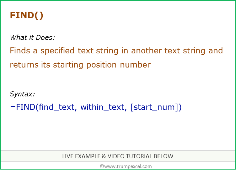
Excel FIND function can be used when you want to locate a text string within another text string and find its position.
What it Returns
It returns a number that represents the starting position of the string you are finding in another string.
Syntax
=FIND(find_text, within_text, [start_num])
Input Arguments
- find_text – the text or string that you need to find.
- within_text – the text within which you want to find the find_text argument.
- [start_num] – a number that represents the position from which you want the search to begin. If you omit it, it starts from the beginning.
Additional Notes
- If the start number is not specified, then it starts looking from the beginning of the string.
- Excel FIND function is case-sensitive. If you want to do a case-insensitive search, use Excel SEARCH function.
- Excel FIND function cannot handle wildcard characters. If you want to use wildcard characters, use the Excel SEARCH function.
- It returns a #VALUE! error if the searched string is not found in the text.
Excel FIND Function – Examples
Here are four examples of using Excel FIND function:
Searching for a Word in a Text String (from the beginning)
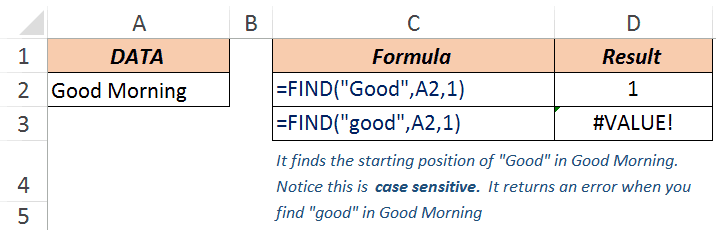
In the above example, when you look for the word Good in the text Good Morning, it returns 1, which is the position of the starting point of the searched word.
Note that Excel FIND function is case-sensitive. When you use good instead of Good, it returns a #VALUE! error.
If you are looking for a case-insensitive search, use Excel SEARCH function.
Finding a Word in a Text String (with a specified beginning)
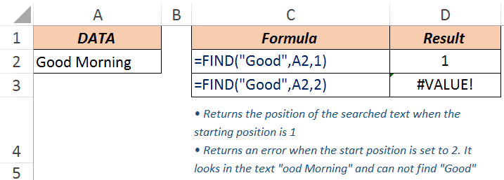
The third argument in the FIND function is the position within the text from where you want to start the search. In the example above, the function returns 1 when you search for the text Good in Good Morning and the starting position is 1.
However, it returns an error when you make it start at 2. Hence, it looks for the text Good in ood Morning. Since it can not find it, it returns an error.
Note: If you skip the last argument and don’t provide the starting position, by default it takes it as 1.
When there are Multiple Occurrence of the Searched Text
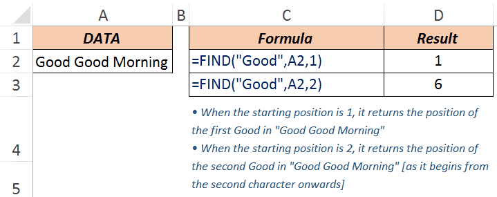
Excel FIND function starts looking in the specified text from the specified position. In the above example, when you look for the text Good in Good Good Morning with the starting position as 1, it returns 1, as it finds it at the beginning.
When you start the search from the second character onwards, it returns 6, as it finds the matching text at the sixth position.
Extracting Everything to the Left a Specified Character/String
Suppose you have the email ids do some superheroes as shown below and you want to extract only the username part (which would be the characters before the @).
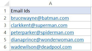
Below is the formula that will find the position of ‘@’ in each email id and extract all the characters to the left of it:
=LEFT(A2,FIND(“@”,A2,1)-1)

The FIND function in this formula gives the position of the ‘@’ character. The LEFT function that uses this position to extract the username.
For example, in the case of brucewayne@batman.com, the FIND function returns 11. LEFT function then uses FIND(“@”,A2,1)-1 as the second argument to get the username.
Note that 1 is subtracted from the value returned by the FIND function as we want to exclude the @ from the result of the LEFT function.
Excel FIND Function – VIDEO
Related Excel Functions:
- Excel LOWER Function.
- Excel UPPER Function.
- Excel PROPER Function.
- Excel REPLACE Function.
- Excel SEARCH Function.
- Excel SUBSTITUTE Function.
You May Also Like the Following Tutorials:
- How to Quickly Find and Remove Hyperlinks in Excel.
- How to Find Merged Cells in Excel.
- How to Find and Remove Duplicates in Excel.
- Using Find and Replace in Excel.
Find in Excel (Table of Contents)
- Using Find and Select Feature in Excel
- FIND Function in Excel
- SEARCH Function in Excel
Introduction to Find in Excel
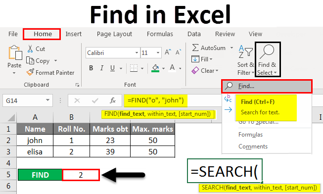
There are two ways to find it in Excel. First, we can use Find by pressing Ctrl + F shortcut keys. Therein Find and Replace box, search the word or field which we want to find in the Find What section. In another way, we can use the FIND function. For this, select the Find function from the insert function and, as per syntax, select the substring from where we need to find it, and choose the word or letter or number which we want to find in the String position. This will return the position of the chosen string from the selected Substring.
Methods to Find in Excel
Below are the different methods to find in excel.
You can download this Find in Excel Template here – Find in Excel Template
Method #1 – Using Find and Select Feature in Excel
Let’s see How to Find a Number or a Character in Excel using the Find and Select feature in Excel.
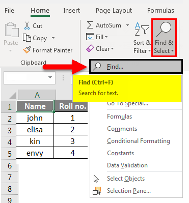
Step 1 – Under the Home tab, in the Editing group, click Find & Select.
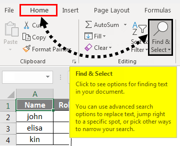
Step 2 – To find text or numbers, click Find.
- In the Find what box, type the text or character you want to search for, or click the arrow in the Find what box and then click a recent search in the list.
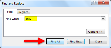
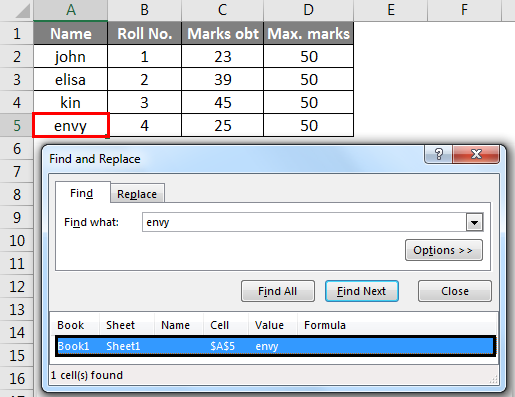
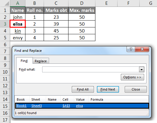
Here, we have a record of marks of four students. Suppose we want to find the text ‘envy’ in this table. For this, we click Find and Select under the Home tab then the Find and Replace dialog box appears. In the Find what box, we enter ‘envy’ then click on Find All. We get the text ‘envy’ is in cell number A5.
- You can use wildcard characters, such as an asterisk (*) or a question mark (?), in your search criteria:
Use the asterisk to find any string of characters.
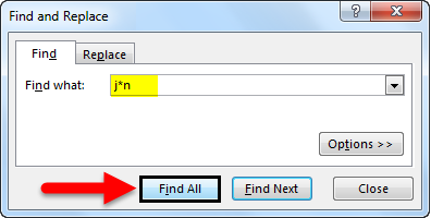
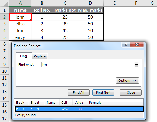
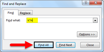
Suppose we want to find text in the table which starts with the letter ‘j’ and ends with the letter ‘n’. In the Find and Replace dialog box, we enter ‘j*n’ in the Find what box, then click on Find All.
We will get the result as text ‘j*n’(john) is in the cell no. ‘A2’ because we have only one text which starts with ‘j’ and ends with ‘n’ with any number of characters between them.
Use the question mark to find any single character.
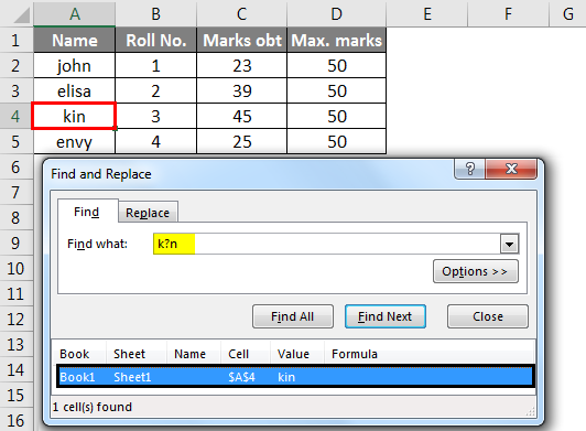
Suppose we want to find text in the table that starts with the letter ‘k’ and ends with the letter ‘n’ with a single character. So, in the Find and Replace dialog box, we enter ‘k?n’ to find what box. Then click on Find All.
Here, we get the text ‘k?n’(kin) is in cell no. ‘A4’ because we have only one text which starts with ‘k’ and ends with ‘n’ with a single character between them.
- Click Options to further define your search if needed.
- We can find text or number by changing settings in the Within, Search and Look in the box according to our needs.
- To show the working of the above-mentioned options, we took the data as follows.
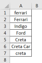
- To search case-sensitive data, select the Match case check box. It gives you output in the case you give input in the Find What box. For example, we have a table of some cars’ names. If you type ‘ferrari’ in the Find What box, then it will find only ‘ferrari’, not ‘Ferrari’.
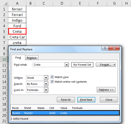
- To search for cells that contain just the characters you typed in the Find what box, select the Match entire cell contents checkbox. For example, we have a table of some cars’ names. Type ‘Creta’ in the Find What box.
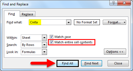
- It will then find cells containing exactly ‘Creta’, and cells containing ‘Cretaa’ or ‘Creta car’ will not be found.
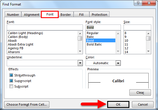
- If you want to search for text or numbers with specific formatting, click Format, and then make your selections in the Find Format dialog box according to your need.
- Let us click the Font option and select the Bold, and click OK.
- Then, we click on Find All.
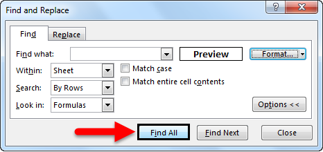
We get the value as ‘elisa’, which is in the ‘A3’ cell.
Method #2 – Using FIND Function in Excel
The FIND function in Excel gives the location of a substring within a string.
Syntax For FIND in Excel:
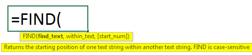
The first two parameters are required, and the last parameter is non-compulsory.
- Find_Value: The substring which you want to find.
- Within_String: The string in which you want to find the specific substring.
- Start_Position: It is a non-compulsory parameter and describes from which position we want to search substring. If you do not describe it, then start the search from the 1st position.
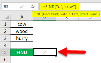
For example =FIND(“o”, “Cow”) gives 2 because “o” is the 2nd letter in the word “cow“.
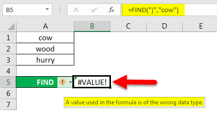
FIND(“j”, “Cow”) gives an error because there is no “j” in “Cow”.
- If the Find_Value parameter contains multiple characters, the FIND function gives the location of the first character.
E.g., the formula FIND(“ur”, “hurry”) gives 2 because “u” in the 2nd letter in the word “hurry”.

- If Within_String contains multiple occurrences of Find_Value, the first occurrence is returned. For example, FIND (“o”, “wood”)
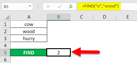
gives 2, which is the location of the first “o” character in the string “wood”.
The Excel FIND function gives the #VALUE! error if:
- If Find_Value does not exist in Within_String.
- If Start_Position contains multiple characters as compared to Within_String.
- If Start_Position either has a zero or negative number.
Method #3 – Using SEARCH Function in Excel
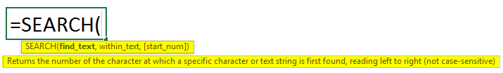
The SEARCH function in Excel is simultaneous to FIND because it also gives the location of a substring in a string.
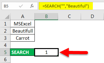
- If Find_Value is the blank string “, the Excel FIND formula gives the string’s first character.
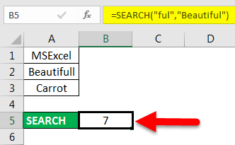
Example =SEARCH (“ful“, “Beautiful) gives 7 because the substring “ful” begins at the 7th position of the substring “beautiful”.
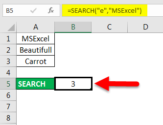
=SEARCH (“e”, “MSExcel”) gives 3 because “e” is the 3rd character in the word “MSExcel” and ignoring the case.
- Excel’s SEARCH function gives the #VALUE! error if:
- If the value of the Find_Value parameter is not found.
- If the Start_Position parameter is superior to the length of Within_String.
- If the Start_Position either equal to or less than 0.
Things to Remember About Find in Excel
- Asterisk defines a string of characters, and the question mark defines a single character. You can also find asterisks, question marks, and tilde characters (~) in worksheet data by preceding them with a tilde character inside the Find what option.
For example, to find data that contain “*”, you would type ~* as your search criteria.
- If you want to find cells that match a specific format, you can delete any criteria in the Find what box and select a specific cell format as an example. Click the arrow next to Format, click Choose Format From Cell, and click the cell with the formatting you want to search for.
- MSExcel saves the formatting options you define; you should clear the formatting options from the last search by clicking on an arrow next to Format and then Clear Find Format.
- The FIND function is case sensitive and does not allow while using wildcard characters.
- The SEARCH function is case-insensitive and allows while using wildcard characters.
Recommended Articles
This is a guide to Find in Excel. Here we discuss how to use the Find feature, Formula for FIND, and SEARCH in Excel, along with practical examples and a downloadable excel template. You can also go through our other suggested articles –
- FIND Function in Excel
- Excel SEARCH Function
- Find and Replace in Excel
- Search For Text in Excel