
Sometimes Excel workbooks become quite large: The more worksheets there are, the more difficult it is to keep the overview. A table of contents might help. In this article we’ll explore 4 ways of creating tables of contents in an Excel workbook.
Let’s say, we want to create a new worksheet with a list of all other worksheets. Furthermore, each list entry should have a link to the corresponding worksheet so that you can easily click on it and will be taken to this worksheet at once. Basically, there are four methods for creating such table of contents: Do it manually, apply a complex formula, use a VBA macro or an Excel add-in.
Method 1: Create a table of contents manually
The first method is the most obvious one: Type (or copy and paste) each sheet name and add links to the cells. These are the necessary steps:
- Create a new worksheet by right clicking on any worksheet name and click on Insert Sheet (or press Shift + Alt + F1). Give a proper name, for example ‘Contents’.
- Start by typing the first worksheet name into cell B4 (or any cell you like…).
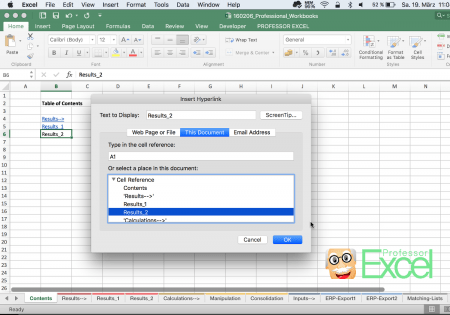
- Add the link to the cell: Right click on the cell and click on ‘Hyperlink’. Select ‘This document’ as shown on the picture above and click on the sheet name you want to create the list entry for. Usually cell A1 is fine as the cell reference. The window of adding a hyperlink on Windows looks a little bit different but offers the same options.
- Repeat steps 2 and 3 until all worksheets are in your table of contents.
- Do all the formatting as desired and then you are done.
Method 2: Use formulas for a table of contents
Thanks to Brian Canes, who posted this method as a comment: There is actually a way of using formulas and named ranges. Follow these steps:
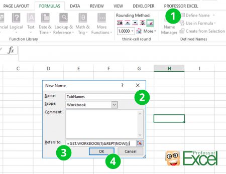
- Click on “Define Name” in the center of the Formulas ribbon.
- Type the name “TabNames”.
- Copy and paste this code into the “Refers to:” field: =GET.WORKBOOK(1)&REPT(NOW(),)
- Confirm with OK.
- Copy this formula into any cell. As it refers to the cell A1, it’ll be the entry for the first worksheet in your workbook:
=IF(ROW(A1)>SHEETS(),REPT(NOW(),),SUBSTITUTE(HYPERLINK("#'"&TRIM(RIGHT(SUBSTITUTE(SUBSTITUTE(INDEX(TabNames,ROW(A1))," ",CHAR(255)),"]",REPT(" ",32)),32))&"'!A1",TRIM(RIGHT(SUBSTITUTE(SUBSTITUTE(INDEX(TabNames,ROW(A1))," ",CHAR(255)),"]",REPT(" ",32)),32))),CHAR(255)," "))
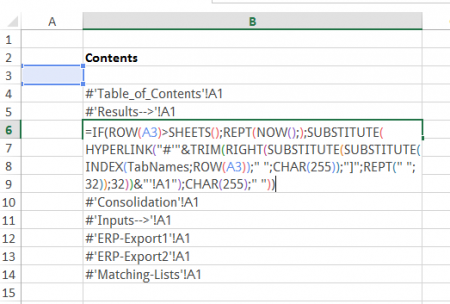
- Copy this formula down until you get blank cells.
Please note:
- All worksheets will be regarded, also hidden ones.
- If you change the order of worksheets, delete some or do any other changes: These changes will be immediately reflected in the table of contents. So you have to be careful if you add comments or do any special formatting.
- You have to save the workbook as a macro enabled workbook in the format “.xlsm”. The reason is that you use a formula as a named range which is only possible with macro-enabled workbooks.
Do you want to boost your productivity in Excel?
Get the Professor Excel ribbon!

Add more than 120 great features to Excel!
Method 3: Use a VBA macro
As the first two methods works but is quite troublesome – especially for large workbooks – we’ll take a look at a third method: A VBA macro. The macro is supposed to do the same steps: Walk through all sheets, create a list entry for each sheet and insert a hyperlink to each sheet.
- Go to the developer ribbon.
- Click on “Editor”.
- Add a new module.
- Paste the following code.
- Press start on the top.
Sub insertTableOfContents()
    Dim PROFEXWorksheet As Worksheet
    Dim tempWorksheetName, tempLink, nameOfTableOfContentsWorksheet As String
    Dim i As Integer

    'Add a new worksheet
    Sheets.Add

    'Rename the worksheet
    nameOfTableOfContentsWorksheet = "TableOfContents"
    ActiveSheet.Name = nameOfTableOfContentsWorksheet

    'Add the headline
    Range("B3") = nameOfTableOfContentsWorksheet

    'Initialize the counting variable i
    i = 0


    'Go through all worksheets as described
    For Each PROFEXWorksheet In Worksheets
            'Copy the current worksheet name
            tempWorksheetName = PROFEXWorksheet.Name

            'Create the link from the current worksheet and link it to cell A1
            tempLink = "'" & tempWorksheetName & "'!R1C1"

            'Add the list entry
            Sheets(nameOfTableOfContentsWorksheet).Cells(i + 5, 2) = tempWorksheetName

            'Select it for inserting the hyperlink
            Sheets(nameOfTableOfContentsWorksheet).Cells(i + 5, 2).Select

            'Insert the hyperlink
            ActiveSheet.Hyperlinks.Add Anchor:=Selection, Address:="", SubAddress:=tempLink

            'Proceed with next entry and increase i therefore
            i = i + 1
    Next
End Sub
Method 4: Use an Excel add-in to create a table of contents
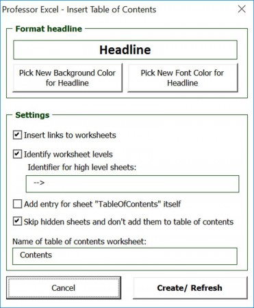
There are some Excel add-ins for creating a table of contents. We – of course – recommend our own add-in. It doesn’t only insert a table of contents but you can easily customize it:
- You can customize the headline color.
- You can choose if you want to insert links to each worksheet.
- You can define levels: For example by high level sheets by their name.
- You can select if you want to insert an entry for the table of contents sheet itself.
- You can choose if you want to skip hidden worksheets or include them as well.
- You can define your preferred name for the table of contents sheets.
Your last settings will be saved so that it’s very fast to update or create a table of contents. There is a free trial version with no sign-up available. Click here to start the download.

This function is included in our Excel Add-In ‘Professor Excel Tools’
(No sign-up, download starts directly)

Henrik Schiffner is a freelance business consultant and software developer. He lives and works in Hamburg, Germany. Besides being an Excel enthusiast he loves photography and sports.
Содержание
- Добавление оглавление в книгу
- Сведения об участниках
- Поддержка и обратная связь
- Insert a table of contents
- Create the table of contents
- If you have missing entries
- Create the table of contents
- If you have missing entries
- Get the learning guide
- Table of Contents in Excel: 4 Easy Ways to Create Directories
- Method 1: Create a table of contents manually
- Method 2: Use formulas for a table of contents
- Method 3: Use a VBA macro
- Method 4: Use an Excel add-in to create a table of contents
- How To Make Table Of Contents In Excel Sheet
- Make Table Of Contents In Excel Sheet
- Method 1: Create A Table Of Contents In Excel Using Hyperlinks
- Method 2: Create Index In Excel Worksheet Using VBA Code
Добавление оглавление в книгу
В следующих примерах показаны различные подходы к добавлению оглавлиния в книгу Excel.
Пример кода, предоставляемый: Деннис Валлентин(Dennis Wallentin), VSTO & .NET & Excel
В этом примере свойство Pages.Count (Excel) используется для вычисления количества страниц на каждом листе. Кроме того, записи в оглавления ссылаться на соответствующие листы для улучшения навигации по книге на экране.
Пример кода, предоставляемый: Билл Jelen, MrExcel.com В этом примере проверяется, существует ли лист с именем «ОГЛА». Если он существует, в примере обновляется оглавление. В противном случае в примере создается новый лист оглавлиения в начале книги. Имя каждого листа вместе с соответствующими номерами печатных страниц указывается в оглавлении. Чтобы получить номера страниц, в примере открывается диалоговое окно Предварительный просмотр. Необходимо закрыть диалоговое окно и создать оглавление.
Сведения об участниках
Деннис Валлентин является автором блога VSTO & .NET & Excel, в который основное внимание уделяется решениям платформа .NET Framework для Excel и службы Excel. Деннис разрабатывает решения Excel более 20 лет и также является соавтором книги «Professional Excel Development: The Definitive Guide to Developing Applications Using Microsoft Excel, VBA, and .NET (2nd Edition)».
Билл Джелен (Bill Jelen), MVP — автор больше двух десятков книг о Microsoft Excel. Он частый гость на TechTV вместе с Лео Лапорте (Leo Laporte) и ведет конференцию MrExcel.com, содержащую больше 300 000 вопросов об Excel и ответов на них.
Поддержка и обратная связь
Есть вопросы или отзывы, касающиеся Office VBA или этой статьи? Руководство по другим способам получения поддержки и отправки отзывов см. в статье Поддержка Office VBA и обратная связь.
Источник
Insert a table of contents
A table of contents in Word is based on the headings in your document.

Create the table of contents
Put your cursor where you want to add the table of contents.
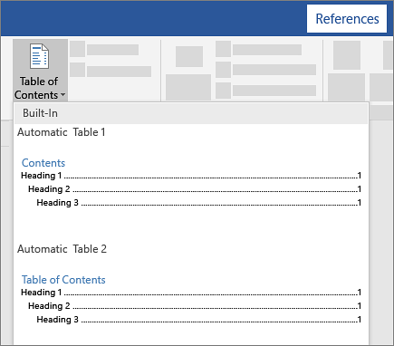
Go to References > Table of Contents. and choose an automatic style.
If you make changes to your document that affect the table of contents, update the table of contents by right-clicking the table of contents and choosing Update Field.
To update your table of contents manually, see Update a table of contents.
If you have missing entries
Missing entries often happen because headings aren’t formatted as headings.
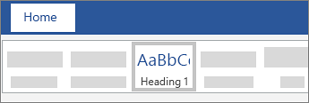
For each heading that you want in the table of contents, select the heading text.
Go to Home > Styles, and then choose Heading 1.
Update your table of contents.
To update your table of contents manually, see Update a table of contents.
Create the table of contents
Word uses the headings in your document to build an automatic table of contents that can be updated when you change the heading text, sequence, or level.
Click where you want to insert the table of contents – usually near the beginning of a document.
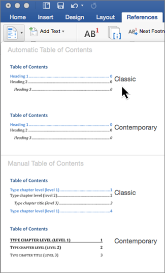
Click References > Table of Contents and then choose an Automatic Table of Contents style from the list.
Note: If you use a Manual Table of Contents style, Word won’t use your headings to create a table of contents and won’t be able to update it automatically. Instead, Word will use placeholder text to create the look of a table of contents so you can manually type each entry into the table of contents. To update your manual table of contents, see Update a table of contents.
If you want to Format or customize your table of contents, you can. For example, you can change the font, the number of heading levels, and whether to show dotted lines between entries and page numbers.
If you have missing entries
Missing entries often happen because headings aren’t formatted as headings.
For each heading that you want in the table of contents, select the heading text.
Go to Home > Styles, and then choose Heading 1.
Update your table of contents.
To update your table of contents manually, see Update a table of contents.
Word uses the headings in your document to build an automatic table of contents that can be updated when you change the heading text, sequence, or level.
Click where you want to insert the table of contents—usually near the beginning of the document.
On the toolbar ribbon, select References.
Near the left end, select Insert Table of Contents. (Or select Table of Contents > Insert Table of Contents.
The table of contents is inserted, showing the headings and page numbering in your document.
If you make changes to your document that affect the table of contents, you can update it by right-clicking the table and selecting Update Table of Contents.
Get the learning guide
For a hands-on guide that steps you through the process of creating a table of contents, download our Table of Contents tutorial. Or, in desktop Word, go to File > New, and search for table of contents.
Источник
Table of Contents in Excel: 4 Easy Ways to Create Directories

Sometimes Excel workbooks become quite large: The more worksheets there are, the more difficult it is to keep the overview. A table of contents might help. In this article we’ll explore 4 ways of creating tables of contents in an Excel workbook.
Let’s say, we want to create a new worksheet with a list of all other worksheets. Furthermore, each list entry should have a link to the corresponding worksheet so that you can easily click on it and will be taken to this worksheet at once. Basically, there are four methods for creating such table of contents: Do it manually, apply a complex formula, use a VBA macro or an Excel add-in.
Method 1: Create a table of contents manually
The first method is the most obvious one: Type (or copy and paste) each sheet name and add links to the cells. These are the necessary steps:
- Create a new worksheet by right clicking on any worksheet name and click on Insert Sheet (or press Shift + Alt + F1). Give a proper name, for example ‘Contents’.
- Start by typing the first worksheet name into cell B4 (or any cell you like…).
- Add the link to the cell: Right click on the cell and click on ‘Hyperlink’. Select ‘This document’ as shown on the picture above and click on the sheet name you want to create the list entry for. Usually cell A1 is fine as the cell reference. The window of adding a hyperlink on Windows looks a little bit different but offers the same options.
- Repeat steps 2 and 3 until all worksheets are in your table of contents.
- Do all the formatting as desired and then you are done.
Method 2: Use formulas for a table of contents
Thanks to Brian Canes, who posted this method as a comment: There is actually a way of using formulas and named ranges. Follow these steps:
- Click on “Define Name” in the center of the Formulas ribbon.
- Type the name “TabNames”.
- Copy and paste this code into the “Refers to:” field: =GET.WORKBOOK(1)&REPT(NOW(),)
- Confirm with OK.
- Copy this formula into any cell. As it refers to the cell A1, it’ll be the entry for the first worksheet in your workbook:
- Copy this formula down until you get blank cells.
- All worksheets will be regarded, also hidden ones.
- If you change the order of worksheets, delete some or do any other changes: These changes will be immediately reflected in the table of contents. So you have to be careful if you add comments or do any special formatting.
- You have to save the workbook as a macro enabled workbook in the format “.xlsm”. The reason is that you use a formula as a named range which is only possible with macro-enabled workbooks.
Do you want to boost your productivity in Excel?
Get the Professor Excel ribbon!
Add more than 120 great features to Excel!
Method 3: Use a VBA macro
As the first two methods works but is quite troublesome – especially for large workbooks – we’ll take a look at a third method: A VBA macro. The macro is supposed to do the same steps: Walk through all sheets, create a list entry for each sheet and insert a hyperlink to each sheet.
- Go to the developer ribbon.
- Click on “Editor”.
- Add a new module.
- Paste the following code.
- Press start on the top.
Method 4: Use an Excel add-in to create a table of contents
There are some Excel add-ins for creating a table of contents. We – of course – recommend our own add-in. It doesn’t only insert a table of contents but you can easily customize it:
- You can customize the headline color.
- You can choose if you want to insert links to each worksheet.
- You can define levels: For example by high level sheets by their name.
- You can select if you want to insert an entry for the table of contents sheet itself.
- You can choose if you want to skip hidden worksheets or include them as well.
- You can define your preferred name for the table of contents sheets.
Your last settings will be saved so that it’s very fast to update or create a table of contents. There is a free trial version with no sign-up available. Click here to start the download.
This function is included in our Excel Add-In ‘Professor Excel Tools’
(No sign-up, download starts directly)
More than 35,000 users can’t be wrong.
Источник
How To Make Table Of Contents In Excel Sheet
As an Amazon Associate and affiliate of other programs, I earn from qualifying purchases.
In this tutorial, we will teach you how you can make a table of contents in the Excel sheets. Without a proper index, it is very hard to manage and navigate a large Excel workbook. However, Excel does not have a built-in feature to create a table of content. But, with the help of the methods shown in this article you can create an index in your Excel worksheet with ease.
Make Table Of Contents In Excel Sheet
To create an index in your worksheet you can make use of hyperlinks. By using the hyperlink you can make it easy to navigate to a particular sheet/content in the workbook by just clicking on its link. And here’s how you can do that.
Method 1: Create A Table Of Contents In Excel Using Hyperlinks
1. Launch Excel on your computer and open the worksheet in which you want to create a table of content. Now, to create an index you will have to insert a new blank page to your already created worksheet. For inserting a new sheet press shift+F11, as you do that a new page will be added to your worksheet.
2. Now you can change the name of the sheet by clicking on it and then select Rename option from the menu

3. Next, select any cell on the sheet and right click on it to open the options menu. Now, select the Hyperlink option.

4. As you do that a new tab will open, on this tab select the option Place in This Document from the left side panel. Now select the content you want to add to the index. The selected content will highlight and the name of the content will be shown on the Text to display box at the top of the tab.

5. Now, remove the cell range( A1 in this case) from the content name on the Text to display box and click then on OK.

6. With this, the content with the hyperlink will be added to the table of content

7. Now you can follow steps 3, 4 and 5 to add remaining content to the table. Once created the hyperlink for all the content your index shall look something like this

Now anyone can easily navigate to all the content on your every worksheet by just clicking on the links. But, this method is not feasible for a very large worksheet because here you have to add content to the table one by one which takes a lot of time. However, there is a second method that can help you create an index for a large worksheet within seconds.
Method 2: Create Index In Excel Worksheet Using VBA Code
VBA stands for Visual Basic for Application. Generally, coders use the VBA editor to create tools for Excel. However, you need not worry if you don’t know how to code because we are going to provide the code. You just have to copy and paste it the editor and you are good to go.
1. Open the Excel worksheet and press Alt + F11 to enter the VBA editor.

2. Now click on Insert from the toolbar at the top and select Module

3. Now copy and paste the following code in the module
Источник
Workbooks that contain large datasets are quite difficult to organize data for navigation. You keep on scrolling and just see tabs expanding wide and you have no idea how many items or products are there in each sheet.
Table of content Excel can help you in this situation, but there is no built-in feature that can directly help you in making content tables for ease. Well, we have come up with a few useful methods to make content tables because larger sheets tend to become uncontrollable.
Let’s get started:
How to Create a Table of Content Excel Manually
In this method, you will follow simple steps without being involved in lengthy procedures.
- Enter each sheet’s name and insert links to the cells. Once this step is done, now lets’ move on to the next part:
- Right-click on the worksheet name and make a new sheet. Choose Insert Sheet and type a valid name there.
- Enter the first sheet name in cell B4.
- Put the link to the cell. For this, right-click on the cell and choose the Hyperlink option.
- Choose This document option and click on the sheet name you need to make the list for.
- Cell A1 would be preferable for reference.
- Now, you need to repeat steps 2 and 3 until each sheet has a table of contents.

How Table of Content Excel is Added with Context Menu
In this method, you will be using the context menu for adding a link. Below are the steps to follow:
- Type the sheet tab name and insert a link. By clicking on the link you will be directed to that particular sheet.
- Once you are done with typing all the sheet’s tabs names, right-click on cell B5.
- The Context Menu will open up.
- Choose the Link option.

- To get the Link option, you can also open the Insert tab from the ribbon and then choose Link from the Links menu.

- The Insert Hyperlink box will be there on the screen.
- Choose Place in This Document from the Link to section.
- Now, set cell reference.
- Choose the place where you need to add a hyperlink.
- Click OK.

- Cell B5 has now added a link.

- The same method will be used to add a link in each cell of your content table.

- Click on any tab and you will be directed to that particular sheet tab.

- If you click on the Australia tab, it will take you to the Australia sheet.
How to Make a Table of Content with VBA Code
Below you will find the VBA code that can help you in making a table of content Excel with links. For this, follow the steps:
Open the Microsoft Visual Basic for Applications window by pressing the ALT + F11 key.
Choose the Insert option and then click on Module. Now, copy the below given VBA code in the Code window.
Sub CreateTableofcontents()
‘updateby Extendoffice 20180413
Dim xAlerts As Boolean
Dim I As Long
Dim xShtIndex As Worksheet
Dim xSht As Variant
xAlerts = Application.DisplayAlerts
Application.DisplayAlerts = False
On Error Resume Next
Sheets(“Table of contents”).Delete
On Error GoTo 0
Set xShtIndex = Sheets.Add(Sheets(1))
xShtIndex.Name = “Table of contents”
I = 1
Cells(1, 1).Value = “Table of contents”
For Each xSht In ThisWorkbook.Sheets
If xSht.Name <> “Table of contents” Then
I = I + 1
xShtIndex.Hyperlinks.Add Cells(I, 1), “”, “‘” & xSht.Name & “‘!A1”, , xSht.Name
End If
Next
Application.DisplayAlerts = xAlerts
End Sub
Press the F5 key and choose the Run button to activate the code.
You will see a table of content Excel in front of all sheets with their names. Click on the sheet name to control the sheet activity.
Summary
You can have a Table of content Excel by using any of the above methods as per your choice. Each method is fairly effective and user-friendly that’s why you don’t need to be worried about it.
In this tutorial, we will teach you how you can make a table of contents in the Excel sheets. Without a proper index, it is very hard to manage and navigate a large Excel workbook. However, Excel does not have a built-in feature to create a table of content. But, with the help of the methods shown in this article you can create an index in your Excel worksheet with ease.
Contents
- 1 Make Table Of Contents In Excel Sheet
- 1.1 Method 1: Create A Table Of Contents In Excel Using Hyperlinks
- 1.2 Method 2: Create Index In Excel Worksheet Using VBA Code
- 1.3 Final Thoughts
To create an index in your worksheet you can make use of hyperlinks. By using the hyperlink you can make it easy to navigate to a particular sheet/content in the workbook by just clicking on its link. And here’s how you can do that.
Method 1: Create A Table Of Contents In Excel Using Hyperlinks
1. Launch Excel on your computer and open the worksheet in which you want to create a table of content. Now, to create an index you will have to insert a new blank page to your already created worksheet. For inserting a new sheet press shift+F11, as you do that a new page will be added to your worksheet.
2. Now you can change the name of the sheet by clicking on it and then select Rename option from the menu
3. Next, select any cell on the sheet and right click on it to open the options menu. Now, select the Hyperlink option.
4. As you do that a new tab will open, on this tab select the option Place in This Document from the left side panel. Now select the content you want to add to the index. The selected content will highlight and the name of the content will be shown on the Text to display box at the top of the tab.
5. Now, remove the cell range( A1 in this case) from the content name on the Text to display box and click then on OK.
6. With this, the content with the hyperlink will be added to the table of content
7. Now you can follow steps 3, 4 and 5 to add remaining content to the table. Once created the hyperlink for all the content your index shall look something like this
Now anyone can easily navigate to all the content on your every worksheet by just clicking on the links. But, this method is not feasible for a very large worksheet because here you have to add content to the table one by one which takes a lot of time. However, there is a second method that can help you create an index for a large worksheet within seconds.
ALSO READ: Convert Picture of Table Into Excel
Method 2: Create Index In Excel Worksheet Using VBA Code
VBA stands for Visual Basic for Application. Generally, coders use the VBA editor to create tools for Excel. However, you need not worry if you don’t know how to code because we are going to provide the code. You just have to copy and paste it the editor and you are good to go.
1. Open the Excel worksheet and press Alt + F11 to enter the VBA editor.
2. Now click on Insert from the toolbar at the top and select Module
3. Now copy and paste the following code in the module
Sub CreateTableofcontents()
Dim xAlerts As Boolean
Dim I As Long
Dim xShtIndex As Worksheet
Dim xSht As Variant
xAlerts = Application.DisplayAlerts
Application.DisplayAlerts = False
On Error Resume Next
Sheets("Table of contents").Delete
On Error GoTo 0
Set xShtIndex = Sheets.Add(Sheets(1))
xShtIndex.Name = "Table of contents"
I = 1
Cells(1, 1).Value = "Table of contents"
For Each xSht In ThisWorkbook.Sheets
If xSht.Name <> "Table of contents" Then
I = I + 1
xShtIndex.Hyperlinks.Add Cells(I, 1), "", "'" & xSht.Name & "'!A1", , xSht.Name
End If
Next
Application.DisplayAlerts = xAlerts
End Sub
4. Run the code by pressing the F5 button or by clicking on the Run button.

5. Next, go to Files and select Close and Return to Microsoft Excel

6. Now you will see the table of content is created with all the hyperlinked content all at once.

Now you can simply click on any of the hyperlinked content to explore it.
Final Thoughts
So that’s how you create a table of content list on Excel for easy navigation of a large worksheet. If you work on Excel then you should definitely learn this skill because it will keep you ahead of all. Also, if you liked our tutorial then do share this article with others as well.
Bottom Line: Learn to create a Table of Contents sheet that automatically updates whenever changes are made to sheets in an Excel workbook.
Skill Level: Intermediate
Download the Excel File
Here’s a link to the file I use in the video that includes the VBA macros.
The following file will work with workbooks that contain Chart sheets. These are NOT worksheets that contain charts. Chart sheets are a special type of sheet that only contains a single chart that takes up the entire sheet.
Chart Sheets cannot be selected with hyperlinks because they do not contain cells. Therefore, this solution uses the Worksheet_FollowHyperlink event to select the Chart sheet. All of the code is still contained in the shtTOC sheet module, and the sheet can be copied to other workbooks.
Create Automatic Updates to Your Table of Contents in Excel
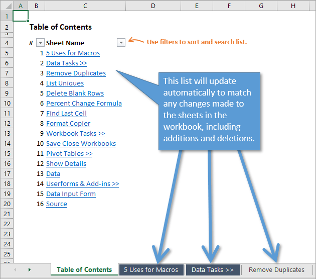
A Table of Contents is a simple yet extremely useful feature in any Excel workbook that contains more than a few sheets. This one sheet can provide a clickable list of your worksheet labels that link directly to their corresponding sheets.
This post will demonstrate how to create a Table of Contents (TOC) that updates automatically. The TOC will display an accurate list when you add, remove, or change the names of sheets in the workbook.
Adding a Macro to Create the Table of Contents
In this example I use two macros to update the Table of Contents.
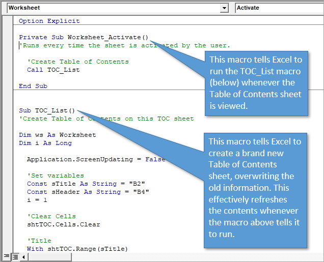
The first macro is the Worksheet_Activate event. This macro will run every time the user selects the Table of Contents sheet. The code is stored in the sheet’s code module, and will only run when that particular sheet is activated (selected).
The code in the Worksheet_Activate calls the second macro (TOC_List). This macro actually recreates the entire Table of Contents on the sheet.
Alternatively, you could put all the code in the TOC_List macro in the Worksheet_Activate event. I just kept them separate in case you want to use a different macro for the TOC, like the TOC Gallery macro I mention below.
You just have to change the Call line in the Worksheet_Activate macro to call a different macro. The macro can also be stored in the same code module for the TOC sheet.
Use it in Your Own Workbooks
This solution is very easy to implement in your own workbooks.
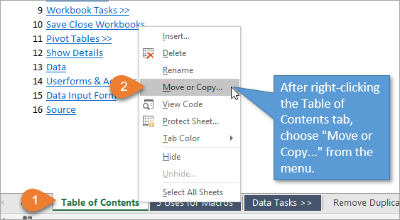
All you have to do is copy the TOC tab (provided in the file download above) to your workbook. All of the code travels with the sheet because it is stored in the sheet’s code module.
Here’s how you can copy the sheet to a different workbook. It’s always a good idea to save your workbook before adding this sheet that contains VBA code.
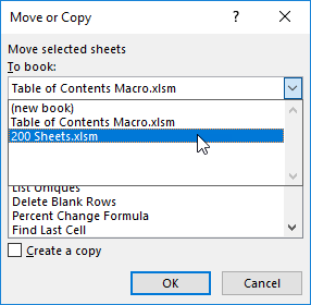
- Right-click on the Table of Contents tab, and then choose “Move or Copy…” in the menu that appears.

- Choose the open workbook that you would like to copy the Table of Contents to. In my example, I am using a workbook called “200 Sheets.”

- Choose the sheet you want the Table of Contents to appear in front of (usually the first sheet since Tables of Contents are normally found at the beginning). Then check the “Create a copy” checkbox. Then select OK.
- The sheet will be copied into the workbook and the Worksheet_Activate event should automatically run to create the new table of contents.

That’s all there is to it. As with any workbook that contains macros, don’t forget to save it as a macro-enabled file (.xlsm extension).
If you’re new to VBA then checkout my free 3-part video series on getting started with macros & VBA.
VBA Code for Automatically Refreshing the Table of Contents
Here is the VBA code for both macros that you can copy and paste into your own workbook. You can also find it in the example Excel file that I’ve provided above.
Sub TOC_List()
'Create Table of Contents on this TOC sheet

Dim ws As Worksheet
Dim wsTOC As Worksheet
Dim i As Long

  Application.ScreenUpdating = False

  'Set variables
  Const bSkipHidden As Boolean = False 'Change this to True to NOT list hidden sheets
  Const sTitle As String = "B2"
  Const sHeader As String = "B4"
  Set wsTOC = Me 'can change to a worksheet ref if using in a regular code module
  i = 1

  'Clear Cells
  wsTOC.Cells.Clear

  'Title
  With wsTOC.Range(sTitle)
    .Value = "Table of Contents"
    .Font.Bold = True
    .Font.Size = .Font.Size + 2

    'List header
    .Offset(2).Value = "#"
    .Offset(2, 1).Value = "Sheet Name"
    .Offset(2).Resize(1, 2).Font.Bold = True
  End With

  'Create TOC list
  With wsTOC.Range(sHeader)

    'Create list
    For Each ws In ThisWorkbook.Worksheets
        'Skip TOC sheet
        If ws.Name <> wsTOC.Name Then
          'Skipping hidden sheets can be toggled in the variable above
          If bSkipHidden Or ws.Visible = xlSheetVisible Then
            .Offset(i).Value = i
            wsTOC.Hyperlinks.Add Anchor:=.Offset(i, 1), _
                                  Address:="", _
                                  SubAddress:="'" & ws.Name & "'!A1", _
                                  TextToDisplay:=ws.Name
            i = i + 1
          End If
        End If
    Next ws

    'Turn filters off
    If wsTOC.AutoFilterMode Then
      wsTOC.Cells.AutoFilter
    End If

    'Apply filters
    .Resize(i, 2).AutoFilter

    'Formatting
    .Font.Italic = True

    'AutoFit
    .Resize(i, 2).Columns.AutoFit

  End With

  Application.ScreenUpdating = True

End Sub
Of course, if you already have a Table of Contents macro that you prefer, you can substitute that code for the TOC_List macro.
How to Skip Hidden Sheets
By default the TOC_List macro will include hidden sheets in the list. However, I added some code to the macro that allows you to skip hidden sheets. This is controlled by the bSkipHidden variable that can be set at the top of the macro.
Here is what that section of code looks like in the macro:
'Set variables
Const bSkipHidden As Boolean = False 'Change this to True to NOT list hidden sheets
  Const sTitle As String = "B2"
It is currently set to False, but you can change it to True to skip hidden sheets. The Table of Contents list will only include the visible sheets in the workbook. Since the macro runs automatically, the Table of Contents will always be updated to display visible sheets only.
Table of Contents Gallery
At the end of the video I show how this same technique can be used with my Table of Contents Gallery macro. If you or your users are more visual-oriented, you might be interested in this solution. Instead of just clickable text, this Table of Contents shows you a snapshot of each sheet in the workbook. Each image is clickable and will take you directly to the corresponding sheet.
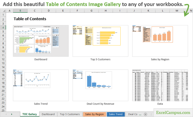
Just a note: This gallery image format does run slower than the list format I described earlier, especially if your workbook has a lot of sheets.
Event-Based Macros
As mentioned before, the Worksheet_Activate event runs any time the user activates the sheet that the code is in. In other words, it’s event based. You can set up macros to run based on other events too, such as:
- Whenever you open or close a workbook.
- Changes are made to any cell, or a particular cell.
- Pivot tables are refreshed.
There are a ton of uses for event macros that will help make your files easier to use. Checkout my post and video on VBA Code Modules & How to Run Macros Based on User Events to learn more.
Professional and User Friendly
Adding a Table of Contents to your workbooks is super easy. And the great thing is that this one feature has the tendency to impress other users (and hopefully your bosses as well!). That’s especially true of the gallery format because it looks like you did so much work!
If you would like to explore some other tips and tricks for making your job easier, making your data look more professional, and making your worksheets more user-friendly, check out my video on 5 uses for VBA macros at your job.
I hope that helps. Please leave a comment below with any questions or suggestions. Thank you! 🙂

Every now and then you are made to work on an Excel workbook that has 15 spreadsheets. It drives you crazy going back and forth those 15 sheets trying to figure out where the information is.
Does this sound familiar ?
Once in a while I work on excel files that have as many as 15 worksheets. In this post, we will see 4 simple ways in which you can stay calm when you have an insanely large workbook with a gazillion worksheets (ok, not gazillion, just a couple of tens of spreadsheets)
1. Excel Table of Contents

When you have lots of sheets, it often helps to build a table of contents spreadsheet with hyperlinks to other sheets. This will help the spreadsheet users to quickly switch between worksheets.
There are 2 ways to do this.
Simple way is to create ToC in Excel is to insert hyperlinks. Press CTRL+k to activate “insert hyperlink” dialog and select “place in this document”. Then select the sheet name and change the “text to display”. Click OK to insert the hyperlink in your workbook. Repeat this for how many ever sheets you have. Now you will have a neat looking table of contents sheet in your workbook.

A slightly elegant way to do this is to use HYPERLINK excel formula. You can write =HYPERLINK(“#’New York’!a1”, “New York”) to insert a link to the New York sheet. When you click on it, excel will take you to the A1 cell in the New York sheet. Remember to use the “#” symbol before the spreadsheet name, otherwise the link wouldn’t work.
2. Use color to differentiate sheets

This is a very good way to know which sheet has what. For eg. you can color all your data sheets in blue and formula / calculation sheets in light yellow. Don’t over color as it looks weird (and that is purely because of Excel’s choice of colors)
3. Learn a few Key Board Shortcuts and Jump Between Sheets Quickly
Use CTRL + Page Down to go to the next spreadsheet
Use CTRL + Page Up to go to the previous spreadsheet
If you know which sheet you need to go, press CTRL + G and type the sheet name along with cell address. For eg. If you need to go to A1 cell in Sheet “London”, type: ‘London’!A1

4. Use the Right Click Menu

This is my favorite trick, right click on the sheet scroll buttons on the lower left corner of the Excel window and select the sheet you want to activate. Click on “More sheets” to see the entire list of sheets and navigate to the one you want.
This post is part of our Spreadcheats series – Learn how to be an Excel Superstar in 31 days, read the rest of the posts in this series.
Photo credit to lorenzo_stupid_kid AKA rockito
Share this tip with your colleagues

Get FREE Excel + Power BI Tips
Simple, fun and useful emails, once per week.
Learn & be awesome.
-
27 Comments -
Ask a question or say something… -
Tagged under
howto, Learn Excel, microsoft, MS, spreadcheats, spreadsheets, table of contents, tips, tricks
-
Category:
Excel Howtos, Featured, Learn Excel

Welcome to Chandoo.org
Thank you so much for visiting. My aim is to make you awesome in Excel & Power BI. I do this by sharing videos, tips, examples and downloads on this website. There are more than 1,000 pages with all things Excel, Power BI, Dashboards & VBA here. Go ahead and spend few minutes to be AWESOME.
Read my story • FREE Excel tips book


Excel School made me great at work.
5/5

From simple to complex, there is a formula for every occasion. Check out the list now.

Calendars, invoices, trackers and much more. All free, fun and fantastic.

Power Query, Data model, DAX, Filters, Slicers, Conditional formats and beautiful charts. It’s all here.

Still on fence about Power BI? In this getting started guide, learn what is Power BI, how to get it and how to create your first report from scratch.
Related Tips
27 Responses to ““Too Many Worksheets” Driving You Nuts? Read This!”
-
 iam_the_maharishi says:
 Or you can use utilities from http://www.asap-utilities.com to create a index worksheet for you. Just click and bang your index worksheet is created at once. The only negative about the util is it forces upgrade twice a year.
-
I wrote an add-in that lets you browse worksheets and switch between them. It’s called Sheet Picker and you can find it on the Add-Ins page on my blog.
-
AndyH says:
Nice tips, as always. Now I wonder when will Excel allow viewing multiple worksheets in separate panes (as you can do with multiple /workbooks/?
-
@Maharishi, JP: thank you for sharing the add-in idea. Personally I have never really used them, but I imagine they would very useful when you work a lot with multiple sheets.
@AndyH: Thank you. Viewing multiple sheets is possible using New windows.
In Excel 2003, press Alt W+N (should work in excel 2007 as well). This creates a new window for the same workbook. Now arrange both windows either vertically or horizontally tiled. Press Alt W+A.
Use different sheets in each window and that is all. Any updates you make will be reflected in both places. -
I personally use your Table of Contents notion…and with Excel you can make a decent TOC at that.
Shot for the third trick! Never knew about that 🙂
I have used ASAP quite a bit…it certainly has decent time saving techniques and then some.
-
I use the first two quite a bit. I never knew about the tip #3, which I will be able to use a lot. Thanks for the tip!
-
@Adam: While I love working on excel, I try to avoid add-ins for multiple reasons (like computer change, security restrictions at work) At home I constantly experiment with add-ins. Never tried the ASAP utility though, I guess I will install it next weekend.
@Tony Rose: You are welcome. Btw, once you specify a range in Go To dialog, it kind of remembers it, so next time you ctrl+G, it shows all the previously «Go to»ed places. Although, this doesn’t seem to work when you go to other sheets.
-
Michael says:
ASAP is excellent. I’ve used it for a year or so. It has some great time savers. I would try each function and then put them in your favorites area.
Also note that you should use the Web toolbar when using hyperlinks … the green back button is helpful in going back and forth — easier than creating a back button or link on each page.
-
Paul says:
I hope this is int he right place…..
I have got all my spreadsheets set up and working, what I want to know is, is there a way to link all the spread sheets together into one nice looking dashboard where the dashboard is automatically updated as I change data in the spreadsheets.
-
@Paul: You are at the right site.. Welcome 🙂
We have put together an excellent set of tutorials, examples and downloads for making excel based dashboards.
You can find them here: http://chandoo.org/wp/management-dashboards-excel
Let me know if you have few more questions…
-
In addition to ctrl + pgup/dn, you can use ctrl + tab or ctrl + shift + tab to move between spreadsheets.
-
@Spotpuff.. thanks alot for sharing this nice tip with us.. Welcome to PHD.. 🙂
-
Magda says:
Hi,
I liked tip #3 until I found out that with more then ca 15 sheets one must click the option «More sheets » and show another even smaller window with annoying scroll bar… Does anyone in MS know what «ergonomy » means?
Is there any way to expand such menus/windows and force them to show all sheets’ names? -
[…] 6: Make ToC (Table of Contents) in Excel – and other tricks […]
-
Mark K says:
Andy H «Nice tips, as always. Now I wonder when will Excel allow viewing multiple worksheets in separate panes (as you can do with multiple /workbooks/?»
In 2007 go to view and click new window.
-
Erin says:
Didn’t know about the ctrl-k shortcut. But then I will admit I have learned only a few of them, ctrl-x, ctrl-c, and ctrl-v being the ones I use 99% of the time.
And this page was #3 in the search results returned by Bing when I Googled!
-
Erin says:
Well, learned one thing — in Excel 2003, the hyperlink dialog box doesn’t see chart sheets (those created by using the chart wizard). And since this is a work project, I can’t use any add-ins that might solve this little wrinkle.
-
[…] Links are achieved by inserting hyperlinks. I choose to reformat these to change the color and remove the underlining. [related: create a table of contents sheet in excel] […]
-
Keggi says:
Hi,
For worksheet’s internal hyperlinks I like to use function since does not whenever I change the name of worksheet:
E.g. (Just Change «Sheet2!A1» and «Link text»)
=HYPERLINK(«#»&CELL(«address»,Sheet2!A1),»Link text») -
I want the user to navigate back to the table of contents for other views as needed so I created a macro to achieve this:
Sub back()
‘
‘ back Macro
‘
Sheets(«Sheet1»).Select
Range(«A1»).Select
End Sub -
@Preet.. it might be even more easier to create a linked text box to first sheet cell a1 and then copy paste it on every other sheet. That way you would have avoided the macro thingie…
-
[…] What to do if you have too many worksheets? […]
-
T.Naga sita ram says:
this site is excelent. i saw this site through google search. it explains neatly
-
[…] The construction of a Table of Contents page was discussed here Table of Contents […]
-
Eva says:
Thanks so much for the post. Saved me in a 60 page exel! Now I’m not looking that much confused :))
-
Philip says:
Hi there
Chandoo’s tip is excellent and started using it.
I was just wondering (and i am not a programmer) if there is a way instead the hyperlink pointing to cell reference A1, to point to the last active cell of the worksheet?
Thank you in advance for anybodys solution -
harish says:
Thanks man!
Leave a Reply
Home/ VBA/ Automatically Create a Table of Contents in Excel
If a workbook contains many sheets you can create a table of contents to make navigating to the sheets easier. This is a fantastic idea when producing a final version of a report in Excel for a customer.
Excel does not yet contain a feature that produces a table of contents, but you can create a macro to get the job done.
This macro will create a new sheet at the start of the workbook named table of contents. If one already exists it will remove it. It will then list the names of all the sheets in the workbook and insert a hyperlink for each one.
Some of the techniques used within this macro include;
- Using a counter loop on the sheets collection to loop through all the sheets of the workbook
- Create and name a sheet during the macro
- Insert hyperlinks for easier navigation of workbook content
- Concatenation of strings for building the hyperlink address and working with a dynamic range
- The ActiveCell object with Offset to move cells
Create a Table of Contents Macro Code
The VBA code is displayed below. Copy and paste it into the module of a workbook where you need a table of contents. This macro is designed to work in a file no matter how many sheets it contains, or what they are called.
Sub CreateTOC()
    Dim i As Byte
    Const SheetName = "Table of Contents"
    With Application
        .ScreenUpdating = False
        .DisplayAlerts = False
    End With
    If Sheets(1).Name = SheetName Then
        Sheets(SheetName).Delete
    End If
    Sheets.Add Before:=Sheets(1)
    Sheets(1).Name = SheetName
    Range("B2").Value = SheetName
    With Range("B2").Font
        .Name = "Calibri"
        .Size = 14
        .Underline = xlUnderlineStyleSingle
        .Bold = True
    End With
    Range("B4").Select
   'Loop through each sheet and create a table of contents using each sheet name
    For i = 2 To Sheets.Count
    ActiveSheet.Hyperlinks.Add Anchor:=Selection, Address:="", SubAddress:=Sheets(i).Name & "!A1", TextToDisplay:=i - 1 & ". " & Sheets(i).Name
    ActiveCell.Offset(2, 0).Select
    Next
    Range("B4:B" & ActiveCell.Row).Font.Underline = xlUnderlineStyleNone
    With Application
        .ScreenUpdating = True
        .DisplayAlerts = True
    End With
End Sub
Reader Interactions
If like me, you create a substantial amount of worksheets in the the one workbook, for certain tasks then a good way to
# 1 help users of the spreadsheet to to navigate your workbook
# 2 give your workbook that professional edge
is to create a Table Of Contents (TOC) on the first worksheet in your Excel workbook.
There is a really quick way to do this in Excel to save you time. Lets get rolling with this great tip… in my example I have renamed my first worksheet as Table Of Contents (TOC), as this is where I am going to put my TOC that will contain the hyperlinks to my other areas of my workbook1. Save your workbook if it has not already been saved. This tip only works with a saved workbook, so if you have just opened a new workbook, and not saved it this won’t work.
- SAVE YOUR WORKBOOK.
- Select the cell you want to LINK TO.
- Point to the cell border, and right click with the mouse.
- Press the ALT key and and drag the cells to the TOC worksheet.
- Once the sheet has been activated you can then drag the cells to position you want the hyperlink to be on the TOC worksheet.
- Release the ALT key and when the pop up menu appears, select “Create Hyperlink Here”

7. The Hyperlink will appear for you with the original cell text.

There it is the quickest way to create a table of contents in Excel.
Let me know if you like this tip.
Do you use table of contents often?.
Other Excel Tip You Might Like.
1. Centre A Title Across An Excel Worksheet.
2. Text Wrapping In Excel
3. Change The Standard Font In Your Excel Workbooks
Want Even More Top Excel Tips?

A How To Excel At Excel Recommended Download.