What is the standard operator for multiplication in an excel формула - Word и Excel

Excel for Microsoft 365 Excel for Microsoft 365 for Mac Excel for the web Excel 2021 Excel 2021 for Mac Excel 2019 Excel 2019 for Mac Excel 2016 Excel 2016 for Mac Excel 2013 Excel 2010 Excel 2007 Excel for Mac 2011 More…Less

Multiplying and dividing in Excel is easy, but you need to create a simple formula to do it. Just remember that all formulas in Excel begin with an equal sign (=), and you can use the formula bar to create them.

Multiply numbers

Let’s say you want to figure out how much bottled water that you need for a customer conference (total attendees × 4 days × 3 bottles per day) or the reimbursement travel cost for a business trip (total miles × 0.46). There are several ways to multiply numbers.

Multiply numbers in a cell

To do this task, use the * (asterisk) arithmetic operator.

For example, if you type =5*10 in a cell, the cell displays the result, 50.

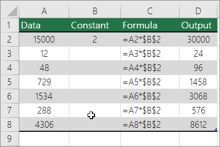
Multiply a column of numbers by a constant number

Suppose you want to multiply each cell in a column of seven numbers by a number that is contained in another cell. In this example, the number you want to multiply by is 3, contained in cell C2.

Type =A2*$B$2 in a new column in your spreadsheet (the above example uses column D). Be sure to include a $ symbol before B and before 2 in the formula, and press ENTER.

Note: Using $ symbols tells Excel that the reference to B2 is «absolute,» which means that when you copy the formula to another cell, the reference will always be to cell B2. If you didn’t use $ symbols in the formula and you dragged the formula down to cell B3, Excel would change the formula to =A3*C3, which wouldn’t work, because there is no value in B3.
Drag the formula down to the other cells in the column.

Note: In Excel 2016 for Windows, the cells are populated automatically.

Multiply numbers in different cells by using a formula

You can use the PRODUCT function to multiply numbers, cells, and ranges.

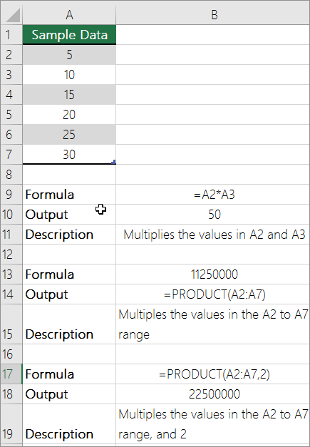
You can use any combination of up to 255 numbers or cell references in the PRODUCT function. For example, the formula =PRODUCT(A2,A4:A15,12,E3:E5,150,G4,H4:J6) multiplies two single cells (A2 and G4), two numbers (12 and 150), and three ranges (A4:A15, E3:E5, and H4:J6).

Divide numbers

Let’s say you want to find out how many person hours it took to finish a project (total project hours ÷ total people on project) or the actual miles per gallon rate for your recent cross-country trip (total miles ÷ total gallons). There are several ways to divide numbers.

Divide numbers in a cell

To do this task, use the / (forward slash) arithmetic operator.

For example, if you type =10/5 in a cell, the cell displays 2.

Important: Be sure to type an equal sign (=) in the cell before you type the numbers and the / operator; otherwise, Excel will interpret what you type as a date. For example, if you type 7/30, Excel may display 30-Jul in the cell. Or, if you type 12/36, Excel will first convert that value to 12/1/1936 and display 1-Dec in the cell.

Note: There is no DIVIDE function in Excel.

Divide numbers by using cell references

Instead of typing numbers directly in a formula, you can use cell references, such as A2 and A3, to refer to the numbers that you want to divide and divide by.

Example:

The example may be easier to understand if you copy it to a blank worksheet.

How to copy an example

Create a blank workbook or worksheet.
Select the example in the Help topic.

Note: Do not select the row or column headers.

Selecting an example from Help
Press CTRL+C.
In the worksheet, select cell A1, and press CTRL+V.
To switch between viewing the results and viewing the formulas that return the results, press CTRL+` (grave accent), or on the Formulas tab, click the Show Formulas button.

	A	B	C
1	Data	Formula	Description (Result)
2	15000	=A2/A3	Divides 15000 by 12 (1250)
3	12

Divide a column of numbers by a constant number

Suppose you want to divide each cell in a column of seven numbers by a number that is contained in another cell. In this example, the number you want to divide by is 3, contained in cell C2.

	A	B	C
1	Data	Formula	Constant
2	15000	=A2/$C$2	3
3	12	=A3/$C$2
4	48	=A4/$C$2
5	729	=A5/$C$2
6	1534	=A6/$C$2
7	288	=A7/$C$2
8	4306	=A8/$C$2

Type =A2/$C$2 in cell B2. Be sure to include a $ symbol before C and before 2 in the formula.
Drag the formula in B2 down to the other cells in column B.

Note: Using $ symbols tells Excel that the reference to C2 is «absolute,» which means that when you copy the formula to another cell, the reference will always be to cell C2. If you didn’t use $ symbols in the formula and you dragged the formula down to cell B3, Excel would change the formula to =A3/C3, which wouldn’t work, because there is no value in C3.

Need more help?

You can always ask an expert in the Excel Tech Community or get support in the Answers community.

For writing formulas, Excel has a standard set of math operators for performing addition, subtraction, multiplication, and exponentiation (raising to the power of). In addition, Excel also provides operators for cell ranges, range intersects, and implicit intersection. The symbols used for these operations are summarized in the table below.

Symbol	Operation	Example
+	Addition	=2+3=5
—	Subtraction	=9-2=7
*	Multiplication	=6*7=42
/	Division	=9/3=3
^	Exponentiation	=4^2=16
()	Parentheses	=(2+4)/3=2
&	Concatenation	=»Z»&100=»Z100″
:	Range	=SUM(F5:F14)=55
space	Range Intersect	=F1:F14 A10:G10 = 6
@	Implicit intersection	@F5:F14 = 10

Logical operators are summarized here. Excel also provides a very large number of built-in functions.

Источник

There is no in-built multiplication formula in Excel. Multiplication in excel is performed by entering the comparison operator “equal to” (=), followed by the first number, the “asterisk” (*), and the second number. In this way, it is possible to carry out the multiplication operation for a cell, row or column. For example, the formula “=16*3*2” multiplies the numbers 16, 3, and 2. It returns 96.

The arithmetic operator “asterisk” (*) is known as the multiplication symbol. It is placed between the numbers to be multiplied.

In multiplication, the number to be multiplied is known as the multiplicand. The number by which the multiplicand is multiplied is known as the multiplier. The multiplier and the multiplicand are also called factors. Their output of multiplication is known as the product.

In Excel, multiplication can be performed in the following ways:

With the “asterisk” symbol (*)
With the PRODUCT functionProduct excel function is an inbuilt mathematical function which is used to calculate the product or multiplication of the given numbers. If you provide this formula arguments as 2 and 3 as =PRODUCT(2,3) then the result displayed is 6.read more
With the SUMPRODUCT functionThe SUMPRODUCT excel function multiplies the numbers of two or more arrays and sums up the resulting products.read more

Note: The SUMPRODUCT function multiplies and then sums the resulting products.

How to Use Multiply Formula in Excel?
- Example #1 – Multiply Excel Columns With the “Asterisk”
- Example #2 – Multiply Excel Rows With the “Asterisk”
- Example #3 – Multiply With the PRODUCT Function
- Example #4 – Multiply and Sum With the SUMPRODUCT Function
- Example #5 – Multiply With Percentages
Frequently Asked Questions
Recommended Articles

How to Use Multiply Formula in Excel?

You can download this Multiply Function Excel Template here – Multiply Function Excel Template

Example #1 – Multiply Excel Columns With the “Asterisk”

The following table shows two columns titled “number 1” and “number 2.” We want to multiply the numerical values of the first column by the second one.

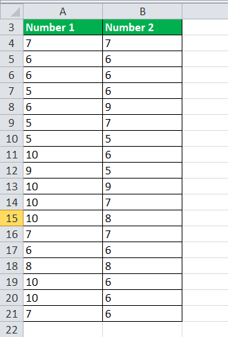
Step 1: Enter the multiplication formula in excel “=A4*B4” in cell C4.

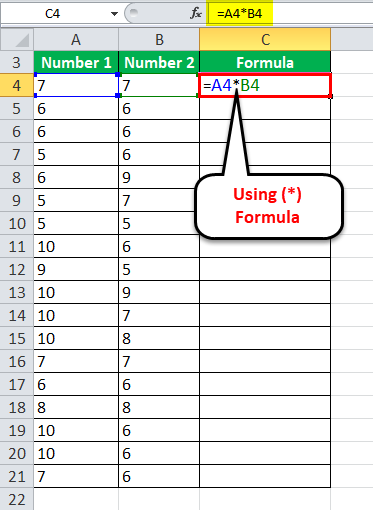
Step 2: Press the “Enter” key. The output is 49, as shown in the succeeding image. Drag or copy-paste the formula to the remaining cells.

For simplicity, we have retained the formulas in column C and given the products in column D.

Example #2 – Multiply Excel Rows With the “Asterisk”

The following table shows two rows titled “number 1” and “number 2.” We want to multiply the numerical values of the first row by the second one.

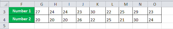
Step 1: Enter the multiplication formula “=G3*G4” in cell G5.

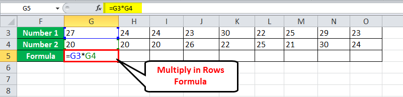
Step 2: Press the “Enter” key. The output is 540, as shown in the succeeding image. Drag or copy-paste the formula to the remaining cells.

For simplicity, we have retained the formulas in row 5 and given the products in row 6.

Example #3 – Multiply With the PRODUCT Function

The PRODUCT function can be given a list of numbers as arguments to be multiplied.

Working on the data of example #1, we want to multiply the numerical values of the two columns with the help of the PRODUCT function.

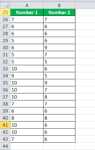
Step 1: Enter the formula “=PRODUCT (A26,B26)” in cell C26.

Step 2: Press the “Enter” key. The output is 49, as shown in the succeeding image. Drag or copy-paste the formula to the remaining cells.

For simplicity, we have retained the formulas in column C and given the products in column D.

Example #4 – Multiply and Sum With the SUMPRODUCT Function

With the SUMPRODUCT function, the numbers of two columns or rows are multiplied and the resulting products are summed up.

The following table shows the prices (in $ per unit) and quantities sold of 20 items. We want to calculate the total sales revenue generated by the organization.

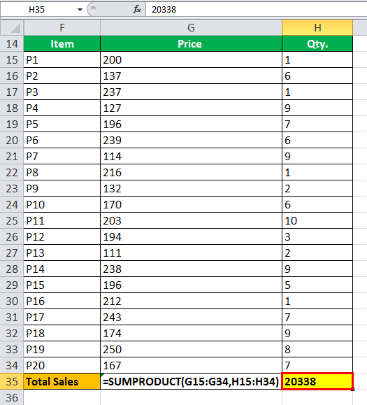
Step 1: Enter the formula “=SUMPRODUCT (G15:G34,H15:H34).”

To calculate the sales revenue, the prices are multiplied by the quantity sold. Thereafter, the resulting products are added by the given formula.

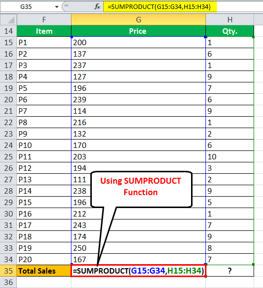
Step 2: Press the “Enter” key. The output is $20,338.

For simplicity, we have retained the formula in cell G35 and given the result in cell H35.

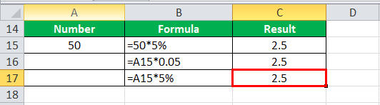
Example #5 – Multiply With Percentages

The following table shows a number in column A. We want to multiply this by 5%.

Step 1: Enter any of the following three formulas:

“=50*5%”
“=A15*0.05”
“=A15*5%”

Step 2: Press the “Enter” key. The output is 2.5 with all the three formulas. It is shown in the following image.

For simplicity, we have retained the formulas in column B and given the results in column C.

Frequently Asked Questions

1. What is the multiplication formula and how to multiply in Excel?

There is no universal formula for multiplication in Excel. However, Excel facilitates multiplication with the use of the “asterisk” (*) and the PRODUCT function.

The formula using the “asterisk” is stated as follows:
“=number 1*number 2”

This is the simplest approach to multiplication that helps multiply numbers, cell references, rows, and columns.

The syntax using the PRODUCT function is stated as follows:

“=PRODUCT(number1,[number2], …)”

The “number1” and “number2” arguments can be in the form of numbers, cell references or ranges. Only the “number1” argument is required.

The steps to multiply in Excel are listed as follows:

• Enter the comparison operator “equal to” (=).
• Enter the multiplication formula.
• Press the “Enter” key to obtain the output.

Note: A maximum of 255 arguments can be provided to the PRODUCT function.

2. How to multiply in Excel without using the formula?

Let us multiply the numbers 4, 15, 23, and 54 (in the range A2:A5) by the constant 2 (in cell B2) without using the formula.

The steps to multiply in excel with “paste special” are listed as follows:
• Select cell B2 and press the keys “Ctrl+C” to copy it.
• Select the range A2:A5, which is to be multiplied.
• Right-click the selected range and choose “paste special.”
• In the “paste special” window, select “multiply” under “operation.”
• Click “Ok.”
The outputs 8, 30, 46, and 108 are obtained in the range A2:A5.

Note: If you do not want the range A2:A5 to be overridden with new values, copy-paste the numbers of this range to a separate column. This is to be done at the beginning of the mentioned procedure.

3. How to multiply two columns in Excel?

Let us multiply column A consisting of 5, 18, 26, and 44 (in the range A2:A5) by column B consisting of 6, 4, 9, and 2 (in the range B2:B5).

The steps to multiply two columns in excel using the multiplication symbol or the PRODUCT formula are listed as follows:

• Enter the formula “=A2*B2” or “=PRODUCT(A2,B2)” in cell C2.
• Press the “Enter” key. The output 30 appears in cell C2.
• Drag or copy-paste the formula to the remaining cells.

The outputs 30, 72, 234, and 88 are obtained in the range C2:C5.

Note: Since relative references are being used, the cell reference changes as the formula is copied.

The steps to multiply two excel columns using the array formula are listed as follows:

• Select the entire range C2:C5 where you want the output.
• Enter the formula “=A2:A5*B2:B5” in the selected range.
• Press the keys “Ctrl+Shift+Enter” together. The curly braces {} appear in the formula bar.

The outputs 30, 72, 234, and 88 are obtained in the range C2:C5.

Multiplication in Excel

To multiply numbers in Excel, we’re going to use the asterisk symbol (*) as the multiplication operator.

Simply follow this multiplication formula =a*b where:

a – the number to be multiplied
b – the number by which it is multiplied

Don’t forget to first type the equal sign (=) in the cell before you type the numbers and the asterisk symbol.

Let’s say you want to multiply the numbers 10 and 5, to do that…

Double-click an empty cell.
Type the multiplication formula =10*5 in the cell or in the formula bar.

First, type the equal sign (=), then the number 10, followed by the asterisk symbol (*), and the number 5.

01 how to multiply in Excel - constant number

Press Enter.

Excel displays 50 as the product.

Easy, right?

Here are other examples of simple multiplication formulas.

03 multiply numbers using Excel formulas

This is super helpful especially when you need to multiply a lot of large numbers.

Or multiply them again and again. The possibilities are endless.

Aside from that, you can also use cell references in the multiplication formulas instead of having to manually type the numbers you want to multiply.

How to multiply cells in Excel

As you know, you can enter and store values in the cells of your Excel spreadsheet.

When you multiply numbers in Excel, instead of typing the numbers one by one, you can just click the cell references of those numbers.

You can find the cell reference in the Name box found to the left of the formula bar.

Let’s multiply cells in Excel.

With the same example as above. Let’s multiply 10 by 5.

Double-click a cell and type the equal sign (=) to start the formula.

You can also start the formula in the formula bar.

05 start all excel formulas with equal sign

Instead of typing 10, click the cell reference which has a cell value of 10.

In our example, it’s cell B3.

Then type the asterisk (*) as the multiplication symbol.

=B3*

Next, instead of typing 5, click the cell reference which has a cell value of 5.

In our example, it’s cell B4.

=B3*B4

Press Enter.

Excel displays 50 as the product result.

Here are other examples of how to multiply in Excel using cell references.

Using cell references in multiplying numbers helps you calculate faster and in a more accurate way.

Not only that you can multiply individual cells but you can also multiply multiple cells.

As long as you know the cell references of the numbers you want to multiply.

Or you can use the PRODUCT function too.

Multiply cells using the PRODUCT function

The PRODUCT function in Excel multiplies all the numbers given as arguments and returns the product.

It can be used to multiply numbers, cell references, and even cell ranges.

The syntax of the PRODUCT function is: PRODUCT(number1, [number2], …) where:

number1 – the first number or range that you want to multiply.
number2 – additional numbers, cells, or ranges that you want to multiply (maximum of 255 arguments)

Let’s multiply two cells using the PRODUCT function.

Double-click a cell and type the equal sign (=) and type the PRODUCT formula.

You can also start the formula in the formula bar.

=PRODUCT(

Select the first cell you want to multiply.

In our example, cell B3. Type a comma(,)

=PRODUCT(B3,

Select the next cell you want to multiply.

In our example, it’s cell B4. Close the formula with a right parenthesis.

=PRODUCT(B3,B4)

Press Enter.

You can also multiply all the cells in one column.

14 how to multiply in excel array formula

You can also multiply cells in two columns.

For example, let’s multiply cells in column B and column C.

14 how to multiply in Excel array formulas

You can also multiply ranges in Excel.

Now, that is how to multiply in Excel using the PRODUCT function.

Amazing, right?

Order of operations

When performing arithmetic operations, it’s important for you to recall and understand the order of operations.

This is not only for Excel but in general.

The order of operations affects the multiplication formula just as it affects other arithmetic operations like addition, subtraction, and division.

The order in which Excel performs operations in formulas is PEMDAS.

PEMDAS stands for Parentheses, Exponents, Multiplication or Division (whichever comes first), Addition or Subtraction (whichever comes first).

Kasper Langmann, Microsoft Office Specialist

For example, in the Excel formula =10*5-3

You need to perform two arithmetic operations: subtraction and multiplication.

Following the PEMDAS, you need to perform first multiplication and then subtraction.

So Excel multiplies 10 by 5 first and then subtracts 3.

Excel then displays 47 as the result.

The table below shows more examples of how the order of operations can impact multiplication formulas.

That’s it – Now what?

You can now let Excel do the math for you after learning how to multiply in Excel.

Learning and practicing how to write Excel formulas will definitely change the game of how you work in Excel. Talk about getting work done faster and easier.

That’s why Excel skills are one of the most needed skills in every job.

Learning Excel can be confusing and overwhelming, but it doesn’t have to be.

Join my FREE Beginner Excel Training to start learning Excel right now, in the right order. You’ll learn the basics of Excel, basic Excel functions, and many more.

It’s easy, quick, and free, just the way you like it.

Alan Anthony Catantan2023-04-03T18:28:52+00:00

Page load link

Источник

This tutorial explains what different symbols mean in formulas in Excel and Google Sheets.

Excel is essentially used for keeping track of data and using calculations to manipulate this data. All calculations in Excel are done by means of formulas, and all formulas are made up of different symbols or operators, depending on what function the formula is performing.

Equal Sign (=)

The most commonly used symbol in Excel is the equal (=) sign. Every single formula or function used has to start with equals to let Excel know that a formula is being used. If you wish to reference a cell in a formula, it has to have an equal sign before the cell address. Otherwise, Excel just shows the cell address as standard text.

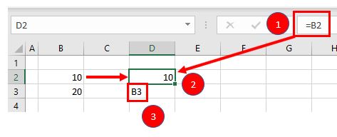
In the above example, if you type (1) =B2 in cell D2, it returns a value of (2) 10. However, typing only (3) B3 into cell D3 just shows “B3” in the cell, and there is no reference to the value 20.

Standard Operators

The next most common symbols in Excel are the standard operators as used on a calculator: plus (+), minus (–), multiply (*) and divide (/). Note that the multiplication sign is not the standard multiplication sign (x) but is depicted by an asterisk (*) while the division sign is not the standard division sign (÷) but is depicted by the forward slash (/).

An example of a formula using addition and multiplication is shown below:

=B1+B2*B3

Order of Operations and Adding Parentheses

In the formula shown above, B2*B3 is calculated first, as in standard mathematics. The order of operations is always multiplication before addition. However, you can adjust the order of operations by adding parentheses (round brackets) to the formula; any calculations between these parentheses would then be done first before the multiplication. Parentheses, therefore, are another example of symbols used in Excel.

=(B1+B2)*B3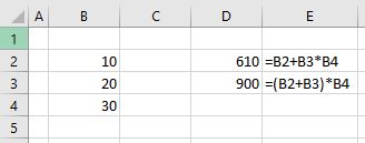

In the example shown above, the first formula returns a value of 610 while the second formula (using parentheses) returns 900.

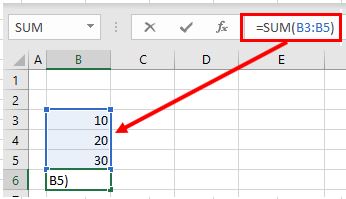
Parentheses are also used with all Excel functions. For example, to sum B3, B4, and B5 together, you can use the SUM Function where the range B3:B5 is contained within parentheses.

=SUM(B3:B5)

Colon (:) to Specify a Range of Cells

In the formula used above, the parentheses contain the cell range which the SUM Function needs to add together. This cell range is expressed with a colon (:) where the first cell reference (B3) is the cell address of the first cell included in the range of cells to add together, while the second cell reference (B5) is the cell address of the last cell included in the range.

Dollar Symbol ($) in an Absolute Reference

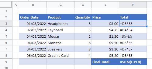
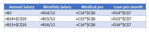
A particular useful and common symbol used in Excel is the dollar sign within a formula. Note that this does not indicate currency; rather, it’s used to “fix” a cell address in place in order that a single cell can be used repetitively in multiple formulas by copying formulas between cells.

=C6*$C$3

By adding a dollar sign ($) in front of the column header (C) and the row header (3), when copying the formula down to Rows 7–15 in the example below, the first part of the formula (e.g., C6) changes according to the row it is copied down to while the second part of the formula ($C$3) stays static always enabling the formula to refer to the value stored in cell C3.

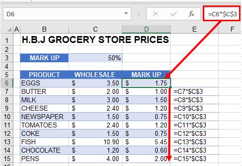
See: Cell References and Absolute Cell Reference Shortcut for more information on absolute references.

Exclamation Point (!) to Indicate a Sheet Name

The exclamation point (!) is critical if you want to create a formula in a sheet and include a reference to a different sheet.

=SUM(Sheet1!B2:B4)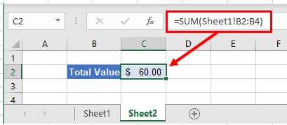

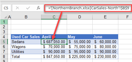
Square Brackets [ ] to Refer to External Workbooks

Excel uses square brackets to show references to linked workbooks. The name of the external workbook is enclosed in square brackets, while the sheet name in that workbook appears after the brackets with an exclamation point at the end.

Comma (,)

The comma has two uses in Excel.

Refer to Multiple Ranges

If you wish to use multiple ranges in a function (e.g., the SUM Function), you can use a comma to separate the ranges.

=SUM(B2:B3, B6:B10)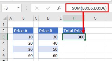

Separate Arguments in a Function

Alternatively, some built in Excel functions have multiple arguments which are usually separated with commas. (These can also be semicolons, depending on the function syntax.)

=VLOOKUP(H5, B6:E15, 4, FALSE)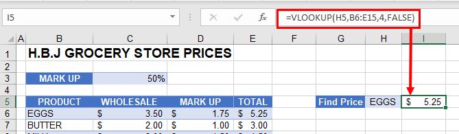

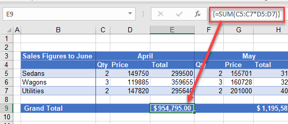
Curly Brackets { } in Array Formulas

Curly brackets are used in array formulas. An array formula is created by pressing the CTRL + SHIFT + ENTER keys together when entering a formula.

Other Important Symbols

Symbol	Description	Example
%	Percentage	=B2%
^	Exponential operator	=B2^B3
&	Concatenation	=B2&B3
>	Greater than	=B2>B3
<	Less than	=B2<B3
>=	Greater than or equal to	=B2>=B3
<=	Less than or equal to	=B2<=B3
<>	Not equal to	=B2<>B3

Symbols in Formulas in Google Sheets

The symbols used in Google Sheets are identical to those used in Excel.

Источник

Multiply numbers

Multiply numbers in a cell

Multiply a column of numbers by a constant number

Multiply numbers in different cells by using a formula

Divide numbers

Divide numbers in a cell

Divide numbers by using cell references

Divide a column of numbers by a constant number

Need more help?

See Also

Need more help?

Want more options?

Table of contents

How to Use Multiply Formula in Excel?

Example #1 – Multiply Excel Columns With the “Asterisk”

Example #2 – Multiply Excel Rows With the “Asterisk”

Example #3 – Multiply With the PRODUCT Function

Example #4 – Multiply and Sum With the SUMPRODUCT Function

Example #5 – Multiply With Percentages

Frequently Asked Questions

Recommended Articles

How to Multiply in Excel: Easy Multiplication Formula

Multiplication in Excel

How to multiply cells in Excel

Multiply cells using the PRODUCT function

Order of operations

That’s it – Now what?

Equal Sign (=)

Standard Operators

Order of Operations and Adding Parentheses

Colon (:) to Specify a Range of Cells

Dollar Symbol ($) in an Absolute Reference

Exclamation Point (!) to Indicate a Sheet Name

Square Brackets [ ] to Refer to External Workbooks

Comma (,)

Refer to Multiple Ranges

Separate Arguments in a Function

Curly Brackets { } in Array Formulas

Other Important Symbols

Symbols in Formulas in Google Sheets