
Excel for Microsoft 365 Excel for Microsoft 365 for Mac Excel for the web Excel 2021 Excel 2021 for Mac Excel 2019 Excel 2019 for Mac Excel 2016 Excel 2016 for Mac Excel 2013 Excel for iPad Excel Web App Excel for iPhone Excel for Android tablets Excel 2010 Excel 2007 Excel for Mac 2011 Excel for Android phones Excel for Windows Phone 10 Excel Mobile More…Less
Operators specify the type of calculation that you want to perform on elements in a formula—such as addition, subtraction, multiplication, or division. In this article, you’ll learn the default order in which operators act upon the elements in a calculation. You’ll also learn that how to change this order by using parentheses.
Types of operators
There are four different types of calculation operators: arithmetic, comparison, text concatenation, and reference.
To perform basic mathematical operations such as addition, subtraction, or multiplication—or to combine numbers—and produce numeric results, use the arithmetic operators in this table.
|
Arithmetic operator |
Meaning |
Example |
|---|---|---|
|
+ (plus sign) |
Addition |
=3+3 |
|
– (minus sign) |
Subtraction |
=3–1 |
|
* (asterisk) |
Multiplication |
=3*3 |
|
/ (forward slash) |
Division |
=3/3 |
|
% (percent sign) |
Percent |
=20% |
|
^ (caret) |
Exponentiation |
=2^3 |
With the operators in the table below, you can compare two values. When two values are compared by using these operators, the result is a logical value either TRUE or FALSE.
|
Comparison operator |
Meaning |
Example |
|---|---|---|
|
= (equal sign) |
Equal to |
=A1=B1 |
|
> (greater than sign) |
Greater than |
=A1>B1 |
|
< (less than sign) |
Less than |
=A1<B1 |
|
>= (greater than or equal to sign) |
Greater than or equal to |
=A1>=B1 |
|
<= (less than or equal to sign) |
Less than or equal to |
=A1<=B1 |
|
<> (not equal to sign) |
Not equal to |
=A1<>B1 |
Use the ampersand (&) to join, or concatenate, one or more text strings to produce a single piece of text.
|
Text operator |
Meaning |
Example |
|---|---|---|
|
& (ampersand) |
Connects, or concatenates, two values to produce one continuous text value. |
=»North»&»wind» |
Combine ranges of cells for calculations with these operators.
|
Reference operator |
Meaning |
Example |
|---|---|---|
|
: (colon) |
Range operator, which produces one reference to all the cells between two references, including the two references. |
=SUM(B5:B15) |
|
, (comma) |
Union operator, which combines multiple references into one reference. |
=SUM(B5:B15,D5:D15) |
|
(space) |
Intersection operator, which produces a reference to cells common to the two references. |
=SUM(B7:D7 C6:C8) |
|
# (pound) |
The # symbol is used in several contexts:
|
|
|
@ (at) |
Reference operator, which is used to indicate implicit intersection in a formula. |
=@A1:A10 =SUM(Table1[@[January]:[December]]) |
The order in which Excel performs operations in formulas
In some cases, the order in which calculation is performed can affect the return value of the formula, so it’s important to understand the order— and how you can change the order to obtain the results you expect to see.
Formulas calculate values in a specific order. A formula in Excel always begins with an equal sign (=). The equal sign tells Excel that the characters that follow constitute a formula. After this equal sign, there can be a series of elements to be calculated (the operands), which are separated by calculation operators. Excel calculates the formula from left to right, according to a specific order for each operator in the formula.
If you combine several operators in a single formula, Excel performs the operations in the order shown in the following table. If a formula contains operators with the same precedence — for example, if a formula contains both a multiplication and division operator — Excel evaluates the operators from left to right.
|
Operator |
Description |
|---|---|
|
: (colon) (single space) , (comma) |
Reference operators |
|
– |
Negation (as in –1) |
|
% |
Percent |
|
^ |
Exponentiation |
|
* and / |
Multiplication and division |
|
+ and – |
Addition and subtraction |
|
& |
Connects two strings of text (concatenation) |
|
= |
Comparison |
To change the order of evaluation, enclose in parentheses the part of the formula to be calculated first. For example, the following formula results in the value of 11, because Excel calculates multiplication before addition. The formula first multiplies 2 by 3, and then adds 5 to the result.
=5+2*3
By contrast, if you use parentheses to change the syntax, Excel adds 5 and 2 together and then multiplies the result by 3 to produce 21.
=(5+2)*3
In the example below, the parentheses that enclose the first part of the formula will force Excel to calculate B4+25 first, and then divide the result by the sum of the values in cells D5, E5, and F5.
=(B4+25)/SUM(D5:F5)
Watch this video on Operator order in Excel to learn more.
How Excel converts values in formulas
When you enter a formula, Excel expects specific types of values for each operator. If you enter a different kind of value than is expected, Excel may convert the value.
|
The formula |
Produces |
Explanation |
|
= «1»+»2″ |
3 |
When you use a plus sign (+), Excel expects numbers in the formula. Even though the quotation marks mean that «1» and «2» are text values, Excel automatically converts the text values to numbers. |
|
= 1+»$4.00″ |
5 |
When a formula expects a number, Excel converts text if it is in a format that would usually be accepted for a number. |
|
= «6/1/2001»-«5/1/2001» |
31 |
Excel interprets the text as a date in the mm/dd/yyyy format, converts the dates to serial numbers, and then calculates the difference between them. |
|
=SQRT («8+1») |
#VALUE! |
Excel cannot convert the text to a number because the text «8+1» cannot be converted to a number. You can use «9» or «8»+»1″ instead of «8+1» to convert the text to a number and return the result of 3. |
|
= «A»&TRUE |
ATRUE |
When text is expected, Excel converts numbers and logical values such as TRUE and FALSE to text. |
Need more help?
You can always ask an expert in the Excel Tech Community or get support in the Answers community.
See Also
-
Basic Math in Excel
-
Use Excel as your calculator
-
Overview of formulas in Excel
-
How to avoid broken formulas
-
Find and correct errors in formulas
-
Excel keyboard shortcuts and function keys
-
Excel functions (alphabetical)
-
Excel functions (by category)
Need more help?
The Excel Formula for Division helps us perform the mathematical division between two numbers, i.e., one is the numerator and the other the denominator.
Excel doesn’t have an inbuilt Division formula. Therefore, we can use the basic method of using the equal “=” sign, and the arithmetic division operator, the forward slash “/”, to divide the values.
Table of Contents
- What Is Excel Formula For Division?
- How To Divide Using Excel Formulas?
- Basic Formula
- Examples
- How To Handle #DIV/0! Error In Excel Divide Formula?
- Important Things To Note
- Frequently Asked Questions
- Download Template
- Recommended Articles
- The Excel Formula for Division helps us divide 2 numeric values.
- We can use the Basic Division method using the arithmetic operator, i.e., by inserting the forward slash “/” in-between the 2 numeric values.
- We have the alternate division method, i.e., the QUOTIENT function, where both the arguments are mandatory and are not non-numeric.
- In case of a “#DIV/0!” error, we must use the IFERROR function to remove the error and replace it with any value according to our wish.
How To Divide Using Excel Formulas?
We can Divide Using Excel Formulas in 2 ways, namely,
- Basic Division Excel formula.
- Quotient Excel formula.
Method #1 – Basic Division Excel Formula
- First, type “=” in an empty cell.
- Next, for Value1, enter the first value or the cell reference holding the value, i.e., the numerator.
- Then, enter the “/” forward slash, i.e., the basic division symbol in Excel.
- Next, for Value2, enter the second value or the cell reference holding the value, i.e., the denominator.
- Finally, press the “Enter” key to execute the formula, and return the calculated result.
Therefore, the Basic Division Excel formula will be “=Value1/Value2”.
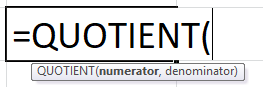
Method #2 – QUOTIENT Excel Formula
The syntax of the QUOTIENT Excel formula is,
The mandatory arguments of the QUOTIENT Excel formula are,
- Numerator: It is the number we are dividing.
- Denominator: It is the numeric value that we are dividing the numerator in excel.
The steps to use the QUOTIENT formula is,
- First, type “=QUOTIENT(” in an empty cell.
- Next, enter the numerator and denominator values as numeric values or cell references.
- Finally, close the brackets and press the “Enter” key to execute the formula.
Basic Formula
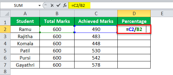
Let us consider an example to use the Excel Formula for Division to divide numbers and calculate the percentages.
We have data of class students who recently appeared in the annual exam. We have the name and total marks they wrote for the exam and the total marks they obtained in the exam.
| Student | Total Marks | Achieved Marks | Percentage |
|---|---|---|---|
| Ramu | 600 | 490 | ? |
| Rajitha | 600 | 483 | ? |
| Komala | 600 | 448 | ? |
| Patil | 600 | 530 | ? |
| Pursi | 600 | 542 | ? |
| Gayathri | 600 | 578 | ? |
The steps to find the percentage of students are:
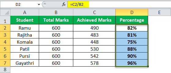
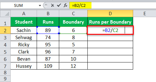
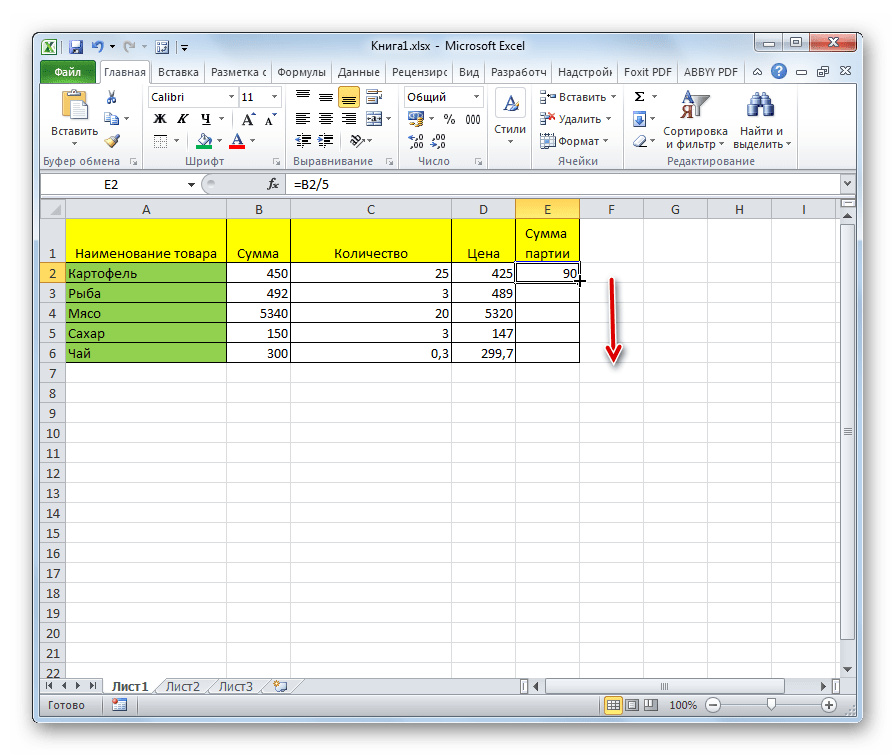
Step 1: Selectcell D2, and enter the formula =C2/B2, i.e., (Achieved Marks / Total Marks).
Step 2: Press the “Enter” key, and drag the formula from cell D2 to D7 using the fill handle. The output, i.e., the percentage of the students, is shown below.
Examples
We will consider a couple of examples using the QUOTIENT Excel Formula for Division.
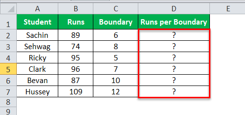
Example #1
We have a cricket scorecard. The individual runs they scored and total boundaries they hit in their innings. We need to find how many runs once they score a boundary. We need to find how many runs once they score a boundary.
The steps to calculate using the QUOTIENT formula are,
Step 1: Select cell D2, enter the formula =B2/C2, press “Enter”, and drag the formula from cell D2 to D7 using the fill handle.

Step 2: Select cell E2, andenter the formula =QUOTIENT(B2,C2).
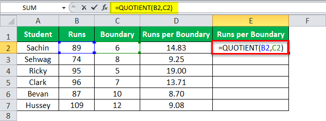
Step 3: Press the “Enter” key, and drag the formula from cell E2 to E7 using the fill handle.
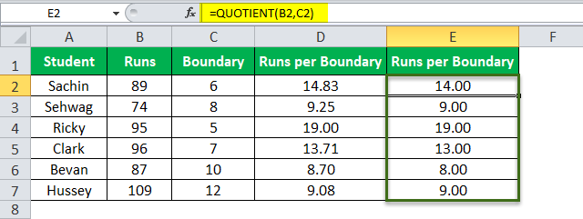
[Note: The QUOTIENT function rounds down the values. However, it will not show the decimal values.]
The output is shown below, i.e., Sachin hits a boundary for every 14th run, Sehwag hits a boundary for every 9th run, etc.
Example #2
Let us consider a scenario of a unique problem.
One day I was busy with my analysis work, and one of the sales managers called and asked if I had an online client. I pitched him for $400,000 plus taxes, but he is asking me to include the tax in the $400,000 itself, i.e., he is requesting the product for $400,000 inclusive of taxes.
We need tax percentage, multiplication rule, and division rule to find the base value.
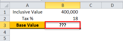
We must apply the Excel formula below to divide what we have shown in the image.
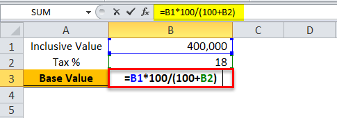
Firstly, the inclusive value is multiplied by 100, and then it is divided by 100 + tax percentage. So, that would give us the base value.
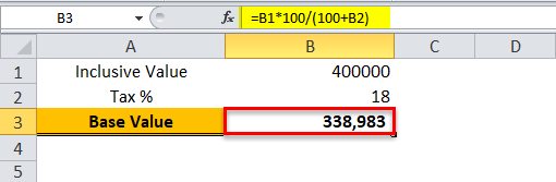
To cross-check, we can take 18% of $338,983, and add a percentage value of $338,983. We should get $400,000 as the overall value.
Sales managers can mention on the contract $338,983 + 18% tax.
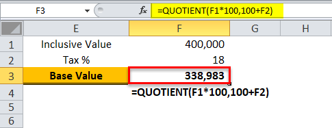
We can also do this by using the QUOTIENT function. The below image is an illustration of the same.
How To Handle #DIV/0! Error In Excel Divide Formula?
In excel, when we are dividing, we get excel errorsErrors in excel are common and often occur at times of applying formulas. The list of nine most common excel errors are — #DIV/0, #N/A, #NAME?, #NULL!, #NUM!, #REF!, #VALUE!, #####, Circular Reference.read more as “#DIV/0!”. This section of the article will explain how to deal with those errors.
We have a five years budget vs. the actual number. So, we need to find out the variance percentages.

The steps to apply the Excel formula to divide are,
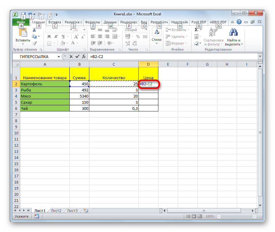
Step 1: Select cell D2, and enter the formula =(B2-C2)/B2.
By deducting the actual cost from the budgeted cost, we get the “Variance Amount”, and then we will divide the “Variance Amount” by the “Budgeted Cost” to get the “Variance Percentage”.

Step 2: Press “Enter”, and drag the formula from cell D2 to D6 using the fill handle. The output is shown below.

Step 3: The problem here is we got an error in the last year, 2018, i.e., cell D6. Since there are no budgeted numbers in 2018, we got #DIV/0! error because we cannot divide any number by zero.
We can eliminate this error by using the IFERROR function in excelThe IFERROR function in Excel checks a formula (or a cell) for errors and returns a specified value in place of the error.read more.
Therefore, select cell D6, enter the formula =IFERROR((B6-C6)/B6,0), and press “Enter”.

The output is shown below. The IFERROR function in Excel converts all the error values to zero.
Important Things To Note
- We get the “#DIV/0!” error if the denominator is zero.
- We get the “#VALUE!” errorif the numerator/denominator or both the values are non-numeric.
- If we type the backward slash “” instead of the forward slash “/”, we get the “#NAME?” error.
- For the QUOTIENT function, both the arguments are mandatory.
Frequently Asked Questions
1) Does Excel have a Division formula?
Excel doesn’t have an inbuilt Division formula. Therefore, we can use the Basic Division Method by using the equal “=” sign, and the forward slash “/” sign to divide the numeric values.
The Basic Division Excel formula will be “=Value1/Value2”.
a) First, type “=” in an empty cell.
b) Next, for Value1, enter the first value or the cell reference holding the value, i.e., the numerator.
c) Then, enter the “/” forward slash, i.e., the basic division symbol in Excel.
d) Next, for Value2, enter the second value or the cell reference holding the value, i.e., the denominator.
e) Finally, press the “Enter” key to execute the formula, and return the calculated result.
2) What is an alternative method for division in Excel?
The alternate method to divide 2 numbers is by using the QUOTIENT formula as follows:
1) First, type “=QUOTIENT(” in an empty cell.
2) Next, enter the numerator and denominator values as numeric values or cell references.
3) Finally, close the brackets and press the “Enter” key to execute the formula.
3) Why is the Division Excel formula not working?
The Division Excel formula may not work for the following reasons,
• If one of the cell values is blank or empty.
• If the values are non-numeric.
• If the denominator is zero.
Download Template
This article must help understand Excel Formula For Division. Here we divide numbers using forward slash “/” operator & QUOTIENT(), examples & a downloadable template. You can download the template here to use it instantly.
You can download this Division Formula Excel Template here – Division Formula Excel Template
Recommended Articles
This article has been a step-by-step guide to Excel Formula For Division Here we discuss how to divide in Excel using the QUOTIENT function and handle #DIV/0! Error, along with practical examples and downloadable templates. You may learn more about Excel from the following articles: –
- Multiply in Excel Formula
- Excel Subtraction Formula
- Matrix Multiplication in Excel
- Percent Error Formula
Содержание
- Способ 1: деление числа на число
- Способ 2: деление содержимого ячеек
- Способ 3: деление столбца на столбец
- Способ 4: деление столбца на константу
- Способ 5: деление столбца на ячейку
- Способ 6: функция ЧАСТНОЕ
- Вопросы и ответы

В Microsoft Excel деление можно произвести как при помощи формул, так и используя функции. Делимым и делителем при этом выступают числа и адреса ячеек.
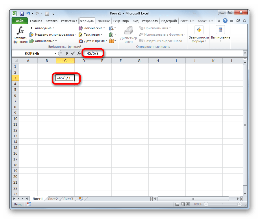
Способ 1: деление числа на число
Лист Эксель можно использовать как своеобразный калькулятор, просто деля одно число на другое. Знаком деления выступает слеш (обратная черта) – «/».
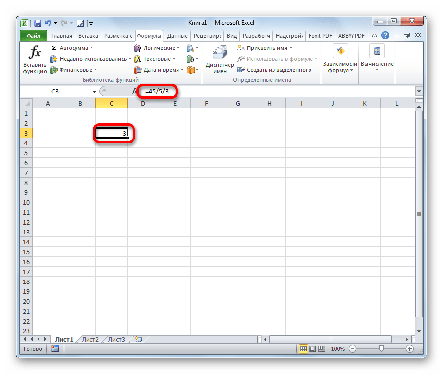
- Становимся в любую свободную ячейку листа или в строку формул. Ставим знак «равно» (=). Набираем с клавиатуры делимое число. Ставим знак деления (/). Набираем с клавиатуры делитель. В некоторых случаях делителей бывает больше одного. Тогда, перед каждым делителем ставим слеш (/).
- Для того, чтобы произвести расчет и вывести его результат на монитор, делаем клик по кнопке Enter.
После этого Эксель рассчитает формулу и в указанную ячейку выведет результат вычислений.
Если вычисление производится с несколькими знаками, то очередность их выполнения производится программой согласно законам математики. То есть, прежде всего, выполняется деление и умножение, а уже потом – сложение и вычитание.
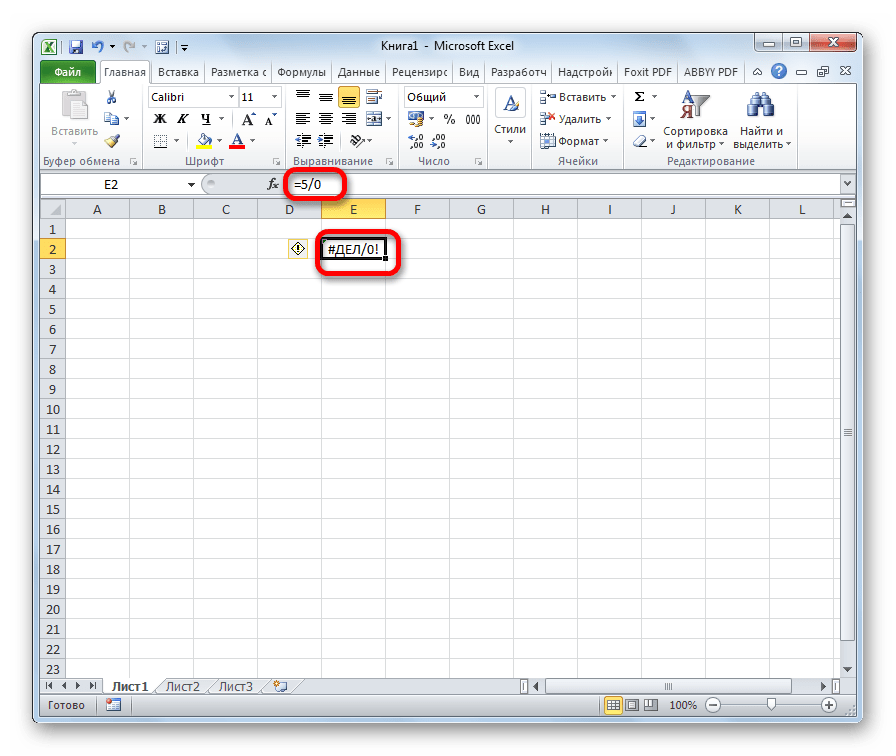
Как известно, деление на 0 является некорректным действием. Поэтому при такой попытке совершить подобный расчет в Экселе в ячейке появится результат «#ДЕЛ/0!».
Урок: Работа с формулами в Excel
Способ 2: деление содержимого ячеек
Также в Excel можно делить данные, находящиеся в ячейках.
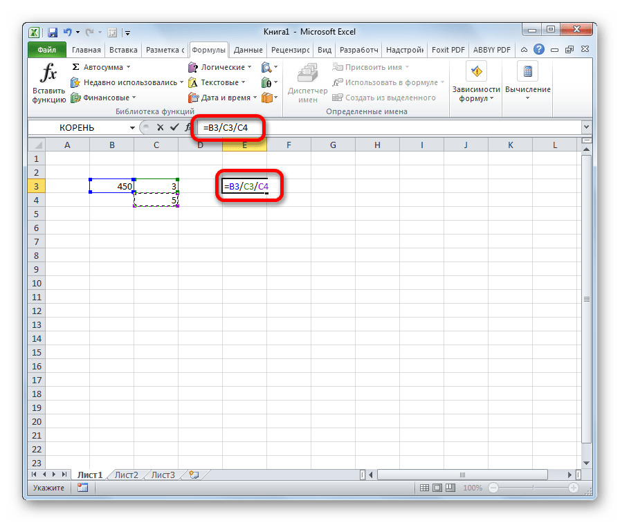
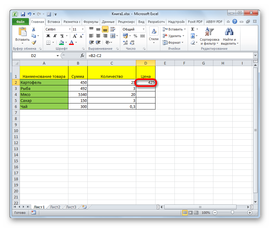
- Выделяем в ячейку, в которую будет выводиться результат вычисления. Ставим в ней знак «=». Далее кликаем по месту, в котором расположено делимое. За этим её адрес появляется в строке формул после знака «равно». Далее с клавиатуры устанавливаем знак «/». Кликаем по ячейке, в которой размещен делитель. Если делителей несколько, так же как и в предыдущем способе, указываем их все, а перед их адресами ставим знак деления.
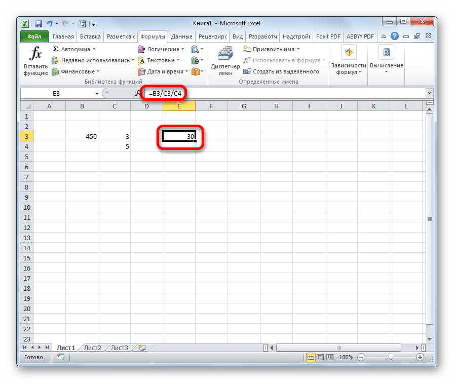
- Для того, чтобы произвести действие (деление), кликаем по кнопке «Enter».
Можно также комбинировать, в качестве делимого или делителя используя одновременно и адреса ячеек и статические числа.
Способ 3: деление столбца на столбец
Для расчета в таблицах часто требуется значения одного столбца разделить на данные второй колонки. Конечно, можно делить значение каждой ячейки тем способом, который указан выше, но можно эту процедуру сделать гораздо быстрее.

- Выделяем первую ячейку в столбце, где должен выводиться результат. Ставим знак «=». Кликаем по ячейке делимого. Набираем знак «/». Кликаем по ячейке делителя.
- Жмем на кнопку Enter, чтобы подсчитать результат.
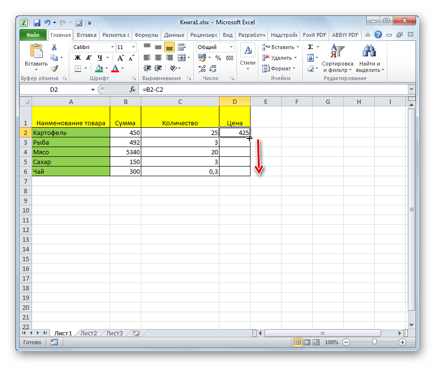
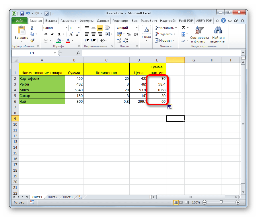
- Итак, результат подсчитан, но только для одной строки. Для того, чтобы произвести вычисление в других строках, нужно выполнить указанные выше действия для каждой из них. Но можно значительно сэкономить своё время, просто выполнив одну манипуляцию. Устанавливаем курсор на нижний правый угол ячейки с формулой. Как видим, появляется значок в виде крестика. Его называют маркером заполнения. Зажимаем левую кнопку мыши и тянем маркер заполнения вниз до конца таблицы.
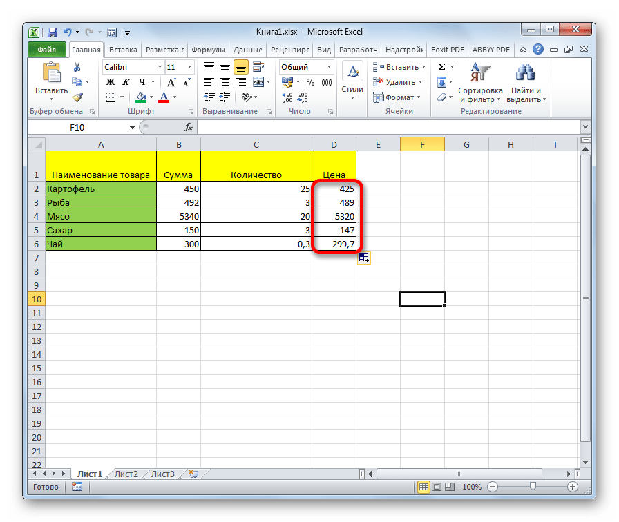
Как видим, после этого действия будет полностью выполнена процедура деления одного столбца на второй, а результат выведен в отдельной колонке. Дело в том, что посредством маркера заполнения производится копирование формулы в нижние ячейки. Но, с учетом того, что по умолчанию все ссылки относительные, а не абсолютные, то в формуле по мере перемещения вниз происходит изменение адресов ячеек относительно первоначальных координат. А именно это нам и нужно для конкретного случая.
Урок: Как сделать автозаполнение в Excel
Способ 4: деление столбца на константу
Бывают случаи, когда нужно разделить столбец на одно и то же постоянное число – константу, и вывести сумму деления в отдельную колонку.
- Ставим знак «равно» в первой ячейке итоговой колонки. Кликаем по делимой ячейке данной строки. Ставим знак деления. Затем вручную с клавиатуры проставляем нужное число.
- Кликаем по кнопке Enter. Результат расчета для первой строки выводится на монитор.
- Для того, чтобы рассчитать значения для других строк, как и в предыдущий раз, вызываем маркер заполнения. Точно таким же способом протягиваем его вниз.


Как видим, на этот раз деление тоже выполнено корректно. В этом случае при копировании данных маркером заполнения ссылки опять оставались относительными. Адрес делимого для каждой строки автоматически изменялся. А вот делитель является в данном случае постоянным числом, а значит, свойство относительности на него не распространяется. Таким образом, мы разделили содержимое ячеек столбца на константу.
Способ 5: деление столбца на ячейку
Но, что делать, если нужно разделить столбец на содержимое одной ячейки. Ведь по принципу относительности ссылок координаты делимого и делителя будут смещаться. Нам же нужно сделать адрес ячейки с делителем фиксированным.
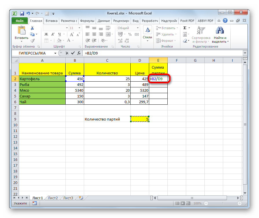
- Устанавливаем курсор в самую верхнюю ячейку столбца для вывода результата. Ставим знак «=». Кликаем по месту размещения делимого, в которой находится переменное значение. Ставим слеш (/). Кликаем по ячейке, в которой размещен постоянный делитель.
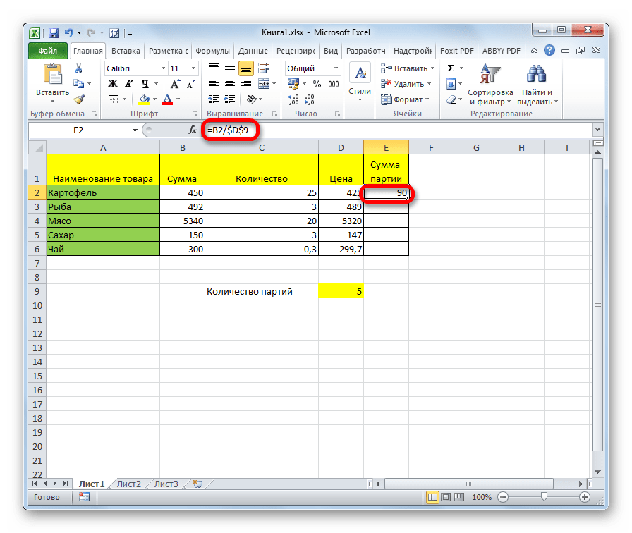
- Для того, чтобы сделать ссылку на делитель абсолютной, то есть постоянной, ставим знак доллара ($) в формуле перед координатами данной ячейки по вертикали и по горизонтали. Теперь этот адрес останется при копировании маркером заполнения неизменным.
- Жмем на кнопку Enter, чтобы вывести результаты расчета по первой строке на экран.
- С помощью маркера заполнения копируем формулу в остальные ячейки столбца с общим результатом.


После этого результат по всему столбцу готов. Как видим, в данном случае произошло деление колонки на ячейку с фиксированным адресом.
Урок: Абсолютные и относительные ссылки в Excel
Деление в Экселе можно также выполнить при помощи специальной функции, которая называется ЧАСТНОЕ. Особенность этой функции состоит в том, что она делит, но без остатка. То есть, при использовании данного способа деления итогом всегда будет целое число. При этом, округление производится не по общепринятым математическим правилам к ближайшему целому, а к меньшему по модулю. То есть, число 5,8 функция округлит не до 6, а до 5.
Посмотрим применение данной функции на примере.
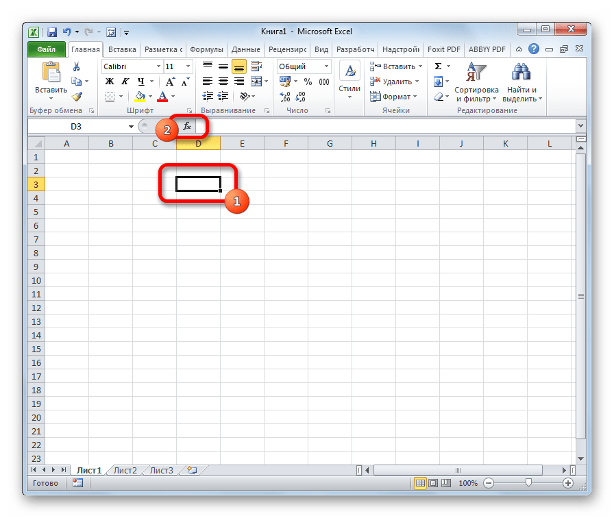
- Кликаем по ячейке, куда будет выводиться результат расчета. Жмем на кнопку «Вставить функцию» слева от строки формул.
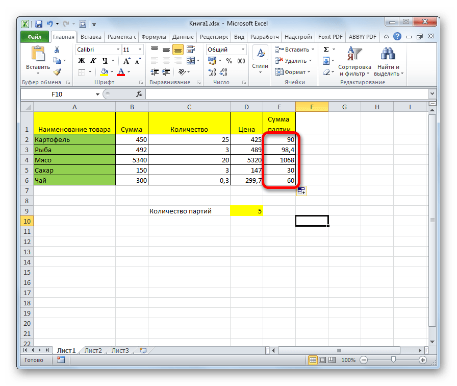
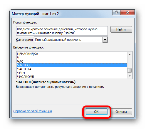
- Открывается Мастер функций. В перечне функций, которые он нам предоставляет, ищем элемент «ЧАСТНОЕ». Выделяем его и жмем на кнопку «OK».
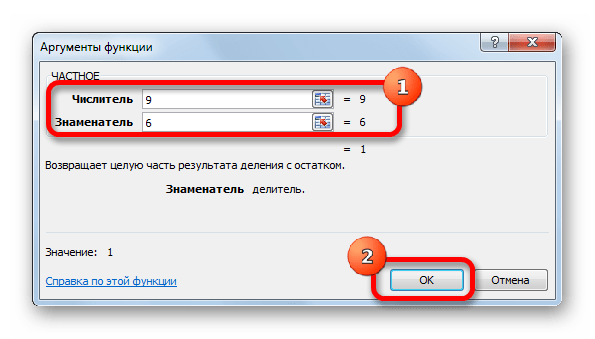
- Открывается окно аргументов функции ЧАСТНОЕ. Данная функция имеет два аргумента: числитель и знаменатель. Вводятся они в поля с соответствующими названиями. В поле «Числитель» вводим делимое. В поле «Знаменатель» — делитель. Можно вводить как конкретные числа, так и адреса ячеек, в которых расположены данные. После того, как все значения введены, жмем на кнопку «OK».
После этих действий функция ЧАСТНОЕ производит обработку данных и выдает ответ в ячейку, которая была указана в первом шаге данного способа деления.
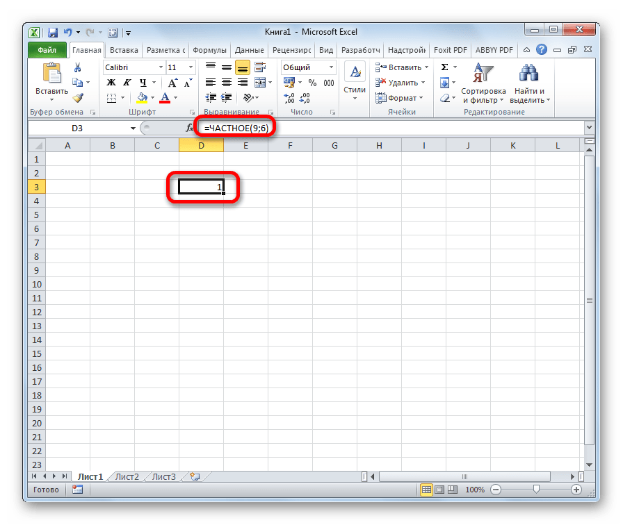
Эту функцию можно также ввести вручную без использования Мастера. Её синтаксис выглядит следующим образом:
=ЧАСТНОЕ(числитель;знаменатель)
Урок: Мастер функций в Excel
Как видим, основным способом деления в программе Microsoft Office является использование формул. Символом деления в них является слеш – «/». В то же время, для определенных целей можно использовать в процессе деления функцию ЧАСТНОЕ. Но, нужно учесть, что при расчете таким способом разность получается без остатка, целым числом. При этом округление производится не по общепринятым нормам, а к меньшему по модулю целому числу.
This time we will venture how to divide division formulas in Excel; we will use examples, syntax, and figures to easy to understand and practice it your perspective.
Microsoft Excel provides different ways how to divide numbers and cells just like in any other basic math operator. It is in your hands what ways you will use considering your preference and requirements of your task. This is the continuation of our tutorial How To Multiply Cells In Excel With Examples.
Additionally, Microsoft Excel is a tool helpful in data entry, management of tasks, recording, and accounting stuff. Therefore a lot of business and work tasks use this application in organizing data and making financial analyses connecting to dividing a load task and finances.
Furthermore, if you use Excel thus encounter mathematical calculations such as division in your worksheet.
What is the Division Formula in Excel
Particularly, Excel does not have a division formula or function, but there are a lot of alternatives we can use. Along with this, you can use an arithmetic operation symbol (/) or a quotient function. Later we will know the things to remember in creating a formula but first, let’s know the syntax…
Syntax
=number1 / number2
It means that the =the number being divided / the number you are dividing by.
Divide symbol
In a division in Excel, the common way to execute it using the division sign. Thus, in arithmetic operations, the division operator uses the obelus symbol (÷) while in excel it uses a forward slash (/) symbol representing it.
Wherefore the expression of this process is written like this =a/b with no spaces where:
- a is the dividend – a number you want to divide, and
- b is the divisor – a number by which the dividend is to be divided.
So here are a few reminders to be kept in mind in creating a formula. This will help you while we jump specifically into dividing in Excel.
- First the equal sign(=). All the formulas must begin with this sign so that Excel will recognize them as formulas.
- Use cell reference. This is where the result of the formula is displayed, not the actual formula. Thus, helpful to enter the data in the cell and if you need to go back to later values, it will be easier to understand.
- Consider PEMDAS (Parenthesis, Exponentiation, Multiplication, Division, Addition, Subtraction) as a reference in the order of arithmetic operations. Below you’ll find an example of how the order of operations is applied to formulas in Excel.
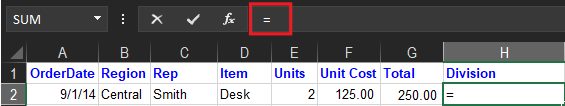
Example 1: Using Numbers Directly
Here’s how to divide in Excel by typing numbers directly into the cell:
- Click the cell where you want the result displayed.
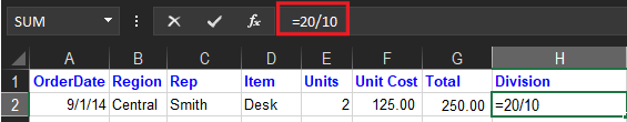
- Type the equal sign(=).
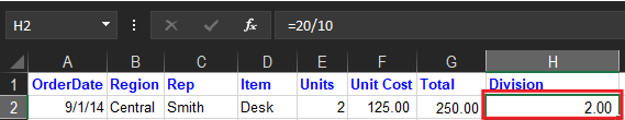
- Create your expression with the operator symbol (/). For instance, if you want to divide 20 by 10, enter 20/10 after the equal sign.
- When you press enter. In the example above, the result would be 2.
Note: Importantly, type equal sign (=) in the cell before you type, the number and the / operator otherwise Excel will read it as date.
For example, if you type 11/10, Excel may display 10-Nov in the cell. Or, if you type 10/20, Excel will first convert that value to 10/30/2020 and display 20-Oct in the cell.
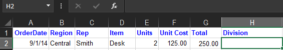
Example 2: Using cell references
Here’s how to divide in Excel by using cell references instead of typing numbers directly into the cell:
- Select the cell where you want the result to appear.
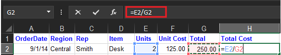
- Type the equal sign, and use cell references instead of typing regular numbers. For instance, if you want to divide cell E2 by cell G2, enter the formula =E2/G2.
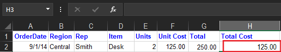
- When you press enter key, Excel displays the result in the cell.
What is the QUOTIENT function in Excel?
The quotient Function is a formula where it divides the two numbers but returns the integer portion of a division. Moreover, it displays a whole number because it discards the rest. For instance, you want to have a quotient of 5 and 2 so the output is 2.5, hence it yields 2 only as the quotient only displays an integer.
How to use the QUOTIENT function in Excel
So here are the steps on how to use QUOTIENT FUNCTION in Excel:
- First, click the cell you want the result to display.
- Enter the =QUOTIENT() into the cell.
- After the parenthesis, type the first number, the dividend, followed by a comma. Then, enter the divisor which is the second number. Then, close the parenthesis.
- It divides numbers in excel when you press enter.
Apparently, the value in the first number or numerator and denominator or second number for a quotient function could be a number, reference cell, cell, or both.
Examples of these are:
- =QUOTIENT(5,2)
- =QUOTIENT(A4,16)
- =QUOTIENT(B2:C3)
Summary
In conclusion, learning how to divide in Excel is very helpful in complying with each task and requirement in business or on daily activities.
Thank you for reading!
For writing formulas, Excel has a standard set of math operators for performing addition, subtraction, multiplication, and exponentiation (raising to the power of). In addition, Excel also provides operators for cell ranges, range intersects, and implicit intersection. The symbols used for these operations are summarized in the table below.
| Symbol | Operation | Example |
|---|---|---|
| + | Addition | =2+3=5 |
| — | Subtraction | =9-2=7 |
| * | Multiplication | =6*7=42 |
| / | Division | =9/3=3 |
| ^ | Exponentiation | =4^2=16 |
| () | Parentheses | =(2+4)/3=2 |
| & | Concatenation | =»Z»&100=»Z100″ |
| : | Range | =SUM(F5:F14)=55 |
| space | Range Intersect | =F1:F14 A10:G10 = 6 |
| @ | Implicit intersection | @F5:F14 = 10 |
Logical operators are summarized here. Excel also provides a very large number of built-in functions.