
Excel for Microsoft 365 Excel 2021 Excel 2019 Excel 2016 Excel 2013 Excel 2010 Excel 2007 Excel Starter 2010 More…Less
Use the Name Manager dialog box to work with all the defined names and table names in a workbook. For example, you may want to find names with errors, confirm the value and reference of a name, view or edit descriptive comments, or determine the scope. You can also sort and filter the list of names, and easily add, change, or delete names from one location.
To open the Name Manager dialog box, on the Formulas tab, in the Defined Names group, click Name Manager.

The Name Manager dialog box displays the following information about each name in a list box:
|
Column Name |
Description |
|---|---|
|
Name |
One of the following:
|
|
Value |
The current value of the name, such as the results of a formula, a string constant, a cell range, an error, an array of values, or a placeholder if the formula cannot be evaluated. The following are representative examples:
|
|
Refers To |
The current reference for the name. The following are representative examples:
|
|
Scope |
|
|
Comment |
Additional information about the name up to 255 characters. The following are representative examples:
|
|
Refers to: |
The reference for the selected name. You can quickly edit the range of a name by modifying the details in the Refers to box. After making the change you can click Commit |


 to save changes, or click Cancel
  to discard your changes.
Notes:
-
You cannot use the Name Manager dialog box while you are changing the contents of a cell.
-
The Name Manager dialog box does not display names defined in Visual Basic for Applications (VBA), or hidden names (the Visible property of the name is set to False).
-
On the Formulas tab, in the Defined Names group, click Define Name.
-
In the New Name dialog box, in the Name box, type the name you want to use for your reference.
Note: Names can be up to 255 characters in length.
-
The scope automatically defaults to Workbook. To change the name’s scope, in the Scope drop-down list box, select the name of a worksheet.
-
Optionally, in the Comment box, enter a descriptive comment up to 255 characters.
-
In the Refers to box, do one of the following:
-
Click Collapse Dialog
 (which temporarily shrinks the dialog box), select the cells on the worksheet, and then click Expand Dialog .
 -
To enter a constant, type = (equal sign) and then type the constant value.
-
To enter a formula, type = and then type the formula.
Tips:
-
Be careful about using absolute or relative references in your formula. If you create the reference by clicking on the cell you want to refer to, Excel will create an absolute reference, such as «Sheet1!$B$1». If you type a reference, such as «B1», it is a relative reference. If your active cell is A1 when you define the name, then the reference to «B1» really means «the cell in the next column». If you use the defined name in a formula in a cell, the reference will be to the cell in the next column relative to where you enter the formula. For example, if you enter the formula in C10, the reference would be D10, and not B1.
-
More information — Switch between relative, absolute, and mixed references
-
-
-
To finish and return to the worksheet, click OK.
 (which temporarily shrinks the dialog box), select the cells on the worksheet, and then click Expand Dialog
  .
.Note: To make the New Name dialog box wider or longer, click and drag the grip handle at the bottom.
If you modify a defined name or table name, all uses of that name in the workbook are also changed.
-
On the Formulas tab, in the Defined Names group, click Name Manager.
-
In the Name Manager dialog box, double-click the name you want to edit, or, click the name that you want to change, and then click Edit.
-
In the Edit Name dialog box, in the Name box, type the new name for the reference.
-
In the Refers to box, change the reference, and then click OK.
-
In the Name Manager dialog box, in the Refers to box, change the cell, formula, or constant represented by the name.
-
On the Formulas tab, in the Defined Names group, click Name Manager.
-
In the Name Manager dialog box, click the name that you want to change.
-
Select one or more names by doing one of the following:
-
To select a name, click it.
-
To select more than one name in a contiguous group, click and drag the names, or press SHIFT and click the mouse button for each name in the group.
-
To select more than one name in a noncontiguous group, press CTRL and click the mouse button for each name in the group.
-
-
Click Delete.
-
Click OK to confirm the deletion.
Use the commands in the Filter drop-down list to quickly display a subset of names. Selecting each command toggles the filter operation on or off, making it easy to combine or remove different filter operations to get the results you want.
You can filter from the following options:
|
Select |
To |
|---|---|
|
Names Scoped To Worksheet |
Display only those names that are local to a worksheet. |
|
Names Scoped To Workbook |
Display only those names that are global to a workbook. |
|
Names With Errors |
Display only those names with values containing errors (such as #REF, #VALUE, or #NAME). |
|
Names Without Errors |
Display only those names with values that do not contain errors. |
|
Defined Names |
Display only names defined by you or by Excel, such as a print area. |
|
Table Names |
Display only table names. |
-
To sort the list of names in ascending or descending order, click the column header.
-
To automatically size the column to fit the longest value in that column, double-click the right side of the column header.
Need more help?
You can always ask an expert in the Excel Tech Community or get support in the Answers community.
See Also
Why am I seeing the Name Conflict dialog box in Excel?
Create a named range in Excel
Insert a named range into a formula in Excel
Define and use names in formulas
Need more help?
What is Name Box in Excel?
The Name Box in Excel is located on the left side of the Excel window. It is used to give a name to a table or any cell. For any normal cells, by default, the name is the row character and the column number, such as cell A1. However, we can check it when we click on the cell. It shows in the Name Box as A1, but we can input any name for the cell, press the “Enter” key, and refer to the cell with the name we put in the Name Box.
Table of contents
- What is Name Box in Excel?
- Where to Find Name Box in Excel?
- How to Use Name Box in Excel?
- #1 – Quick & Fast to go to the Specific Cell
- #2 – Select More than Once Cell at a Time
- #3 – Select Range of Cells From Active Cell
- #4 – Select only Two cells
- #5 – Select Multiple Range of Cells
- #6 – Select Entire Column
- #7 – Select Entire Row
- Recommended Articles
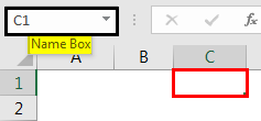
A Name Box is a tool that shows the active cell address. For example, if you have selected cell C1, this Name Box will show the active cell address as C1.
- The first scenario in Excel is when we are working with Excel by mistake; we would press some other key from the keyboard. Suddenly our active cell goes missing, and we do not know what the active cell is now. How do you find what is the active cell now?
- The second one is that we have seen most people use a range of cells as referenceCell reference in excel is referring the other cells to a cell to use its values or properties. For instance, if we have data in cell A2 and want to use that in cell A1, use =A2 in cell A1, and this will copy the A2 value in A1.read more for their formulas when we can use named ranges easily without worrying about the wrong range of cells selection and finding the range of cells in the large worksheet.
Both of the above seem like bigger problems, but the solutions are as simple. The solution for both scenarios is “Name Box.” This article will take you through the tool “Name Box.”
Where to Find Name Box in Excel?
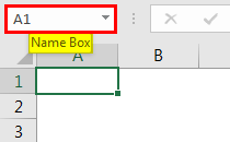
The “Name Box” is available at the Excel Formula bar’s left end. Even though we work enough time with Excel spreadsheets, it goes unnoticed by many of the users.
How to Use a Name Box in Excel?
The usage of the Name Box is not only limited to active cell addresses, but it has many more features which can be critical in daily use. So, now we will see what this name box uses.
#1 – Quick & Fast to go to the Specific Cell
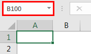
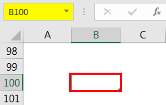
It is one of the great features when we work with large databases. So we often return to the specific cells to do the job. For example, assume you want to go to cell B100. It will take a lot of time to reach that cell if we scroll down the worksheet. But using the name box, we can quickly locate and arrive at that cell.
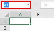
- For this, first, we must select the “Name Box.”

- Now, type the cell address that we want to go to.

- After typing the desired cell address, press the “Enter” key. It will take you to the mentioned cell.

#2 – Select More than Once Cell at a Time
Assume you have data like the below picture.
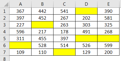
In this data, we have blank cells. Therefore, if we want to select the full data range, using the shortcut Shift + Ctrl + Right Arrow keys from cell A1, it will choose until it finds the blank cell, i.e., until cell D1.
Similarly, for the shortcut key Shift + Ctrl + Down Arrow, it will stop at the A6 cell.
In such cases, the more blank cells, the more time it takes, and it is frustrating because of irritating empty cells. To quickly select this range of cells, we can enter the range of cells in the name box itself.
In this case, our first cell selected is A1, and the last cell is E7. So, we must type the cell address range as A1:E7 in the name box, then press the “Enter” key. It will select the mentioned range of cells quickly.
#3 – Select Range of Cells From Active Cell
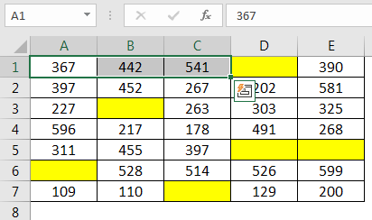
Assume your active cell is B3. You want to select the range of cells from this cell as B3:D6.
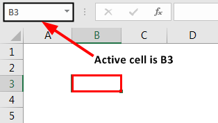
We need not mention the range of cells as B3:D6. Rather than from the active cell, insert the end of the cell address range. Then, in the name box, type the last cell to be selected, the D6 cell.
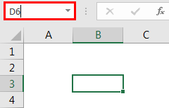
Do not press the “Enter” key. Rather, press the Shift + Enter key to select the range of cells.
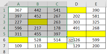
#4 – Select only Two cells
In the above example, we have selected a range of cells. From active cell B3, we have entered D6 as the last cell of the range and hit Shift + Enter to select the range as B3 to D6. But instead of pressing Shift + Enter,if we press Ctrl + Enter, it will choose only two cells, B3 and D6.

Now, press the Ctrl + Enter keys to select two cells, B3 and D6.
#5 – Select Multiple Range of Cells
In the above two examples, we have seen how to select a range of cells from active cells and two individual cells. Now, we will see how to select multiple ranges of cells. For example, look at the below data.
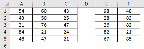
In the above image, we have two sets of ranges one is from A1 to C5, and another one is from E1 to F5. We can select two different ranges of cells from the name box. Enter two ranges of cells separated by a comma (,).
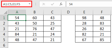
After entering the range address, press the “Enter” key or “Ctrl + Enter” to select the range of cells as mentioned.
#6 – Select Entire Column
We can also select the entire column from the name box. For example, if we want to choose the whole column C, then type the address as C:C.
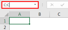
Press the “Enter” key after you mention the column address.
#7 – Select Entire Row
We can also select the entire row from the name box. For example, if we want to choose the whole row 2, then type the address as 2:2.
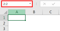
Press the “Enter” key after you mention the row address.
Like this, we can use the Excel Name Box to our advantage at our workplace to work efficiently.
Recommended Articles
This article is a guide to Name Box in Excel. We discuss using the name box property to find the active cell address and select the entire range of cells, rows, and columns in Excel, along with practical examples and a downloadable Excel template. You may learn more about Excel from the following articles: –
- Compare and Match Excel ColumnsThe users can compare and match two columns in excel as per their requirements, data structure and the tools known by applying different formulas. One such example is comparing and matching two excel columns to get the result as «TRUE» and «FALSE».read more
- Excel AVERAGEIFS FunctionWhen there are multiple conditions to be met, the AVERGAEIFS function in Excel is used to find the average from the target range of cells. We used AVERGAEIF for a single condition, but AVERGAEIFS for multiple conditions.read more
- What is Excel Dynamic Named Range?Dynamic named range in excel changes as the data in the range changes, and so does the dashboard or charts or reports associated with them. To make a table as a dynamic named range, select the data, insert a table, and then name the table.read more
- Name Range in ExcelName range in Excel is a name given to a range for the future reference. To name a range, first select the range of data and then insert a table to the range, then put a name to the range from the name box on the left-hand side of the window.read more
- Row Limit in ExcelLimit of rows in excel is a great tool to add more protection to the spreadsheet as this limits the other users to change or modify the spreadsheet to an extensive limit.read more
In Microsoft Excel, the Name Box is located next to the formula bar above the worksheet area. Its regular job is to display the cell reference of the active cell, but it’s also used to name and identify ranges of selected cells or other objects, select one or more ranges of cells in a worksheet, and navigate to different cells in a worksheet or workbook.
Instructions in this article apply to Excel 2019, 2016, 2013, and 2010, as well as Excel for Microsoft 365, Excel for Mac, and Excel Online.
Name and Identify Cell Ranges
When you use the same group of cells in formulas and charts, define a name for the range of cells to identify that range.
To adjust the size of the Name Box, drag the ellipses (the three vertical dots) located between the Name Box and the Formula Bar.
To define a name for a range using the Name Box:
-
Select a cell in a worksheet, such as B2.
To apply a range name to multiple cells, select a contiguous group of cells.
-
Type a name, such as TaxRate.
-
Press Enter to apply the range name.
-
Select the cell in the worksheet to display the range name in the Name Box.
If the range includes multiple cells, select the entire range to display the range name in the Name Box.
-
Drag across a range of multiple cells to display the number of columns and rows in the Name Box. For example, select three rows by two columns to display 3R x 2C in the Name Box.
-
After you release the mouse button or Shift key, the Name Box displays the reference for the active cell, which is the first cell selected in the range.
Name Charts and Pictures
When charts and other objects, such as buttons or images, are added to a worksheet, Excel automatically assigns a name. The first chart added is named Chart 1, and the first image is named Picture 1. If your worksheet contains several charts and pictures, give these images descriptive names to make these images easier to find.
To rename charts and pictures:
-
Select the chart or image.
-
Place the cursor in the Name Box and type a new name.
-
Press Enter to complete the process.
Select Ranges with Names
The Name Box selects or highlights ranges of cells, using either defined names or by entering the cell references. Type the name of a defined range into the Name Box, and Excel selects that range in the worksheet.
The Name Box has an associated dropdown list that contains all the names that have been defined for the current worksheet. Select a name from this list and Excel selects the correct range.
The Name Box also selects the correct range before carrying out sorting operations or before using certain functions such as VLOOKUP, which require the use of a selected data range.
Select Ranges With References
Select an individual cell by typing its cell reference into the Name Box and pressing the Enter key, or highlight a contiguous range of cells using the Name Box.
-
Select the first cell in the range to make it the active cell, such as B3.
-
In the Name Box, type the reference for the last cell in the range, such as E6.
-
Press Shift+Enter to highlight all cells in the range, for example B3:E6.
Select Multiple Ranges
Select multiple ranges in a worksheet by typing them into the Name Box. For example:
- Type D1:D15, F1: F15 into the Name Box to highlight the first 15 cells in columns D and F.
- Type A4:F4, A8:F8 to highlight the first six cells in rows four and eight.
- Type D1: D15, A4:F4 to highlight the first 15 cells in column D and the first six cells in row four.
Select Intersecting Ranges
When you want to select the portion of the two ranges that intersect, separate the identified ranges with a space instead of a comma. For example, type D1: D15 A4:F12 into the Name Box to highlight the range of cells D4:D12, which are the cells common to both ranges.
If names are defined for the ranges, use the named ranges instead of the cell references.
For example, if the range D1:D15 is named test and the range F1:F15 is named test2, type test, test2 in the Name Box to highlight the ranges D1:D15 and F1:F15.
Select Entire Columns or Rows
Select adjacent columns or rows using the Name Box, for example:
- Type B:D to highlight every cell in columns B, C, and D.
- Type 2:4 to select every cell in rows 2, 3, and 4.
Navigate the Worksheet
The Name Box also provides a quick way to navigate to a cell or range in a worksheet. This approach saves time when working in large worksheets and eliminates the need to scroll past hundreds of rows or columns.
-
Place the cursor in the Name Box and type the cell reference, for example, Z345.
-
Press Enter.
-
The active cell highlight jumps to the cell reference, for example, cell Z345.
Jump to a Cell Reference
There’s no default keyboard shortcut for placing the cursor (the blinking insertion point) inside the Name Box. Here’s a faster method to jump to a cell reference:
-
Press F5 or Ctrl+G to open the Go To dialog box.
-
In the Reference text box, type the cell reference or defined name.
-
Select OK or press Enter key to go to the desired location.
Thanks for letting us know!
Get the Latest Tech News Delivered Every Day
Subscribe
Very simply put, the Name Box is a name-displaying tool. Selection of any cell, column, row, named range, chart, picture, etc., (any item on the worksheet window) shows its name in the Name Box.
Displaying the name by selection of any cell or item is the prime job of the Name Box but note that it’s just the prime job. The Name Box can be used as a selection and navigation tool in a workbook. How? Let this tutorial show you.

Location of the Name Box
The Name Box is nestled below the ribbon menu, above the worksheet window, and to the left of the formula bar. To jump to the Name Box, press Alt + F3.

The size of the Name Box (and consequently the size of the formula bar too) can be adjusted by clicking on vertical ellipses (3 dots) on the right of the Name Box and moving it left and right.
Uses of Name Box
Now that we know where it sits and what it is, let’s find out what good that Name Box is for.
1. Displaying Names
Most of you would already be knowing that the Name Box is most commonly used for displaying cell addresses or names. Let’s see what else does it do:
a) Displays the Address of the Active Cell
The simplest and most straightforward use of a Name Box is to show the address of the active cell.

For instance, here we have selected cell B2 and the name box displays its address.
b) Displays the Selected Number of Rows and Columns While Making a Selection
While selecting a range of cells (while the mouse or shift key is held), the Name Box will display the number of rows and columns that are being selected.

Once the mouse or shift key is released and the selection is made, the Name box displays the first selected cell.
c) Displays the Name of the Selected Named Range
The range B3:G18 has been named Sales. Selecting it will show the name of the range (i.e. Sales) in the Name Box.

d) Displays the Name of a Named Cell
Cell I3 has been named GST. Selecting this cell will show GST instead of I3 in the Name Box.

e) Displays the Name of the Selected Named Objects
The Name box will display the name of any selected picture, chart, checkbox, or any named object. The inserted chart has automatically been named Chart 1. Selecting the chart shows the name in the Name Box.

2. Naming Cells, Ranges, or Objects Using Name Box
Let’s see how Name Box can assist you in naming cells or cell ranges.
a) The Name Box can be Used to Name a Cell
By default, the name of a cell is its address (e.g. A1). The name of a cell can be changed from the Name Box. Click on the Name Box, enter a new name for the cell, press Enter.

Similarly, select any row or column, enter a name in the Name Box, and hit Enter.
b) The Name Box can be Used to Name a Range (Creating a Named Range)
Just the way you would rename a cell but for a named range, you select the range. Click on the Name Box, enter a name for the range, press Enter.
c) The Name Box can be Used to Rename an Object in the Sheet
Objects already have names e.g. Table1, Chart1, Picture1 etc. When the object is selected, the name of the object appears in the Name Box. Click on the Name Box, rename the object, and press Enter.

Recommended Reading: All About Named Ranges In Excel
3. Navigation Using Name Box
Cell or Range navigation is another prominent feature of the Name Box. Let’s see different ways in which Name Box helps in navigation.
a) Navigate to Any Cell
Select the Name Box, type the cell reference you want to go to, hit Enter. Let’s use the Name Box to navigate to cell C9.

b) Navigate to Multiple Cells
Multiple cells can be selected by clicking on one cell and typing the other cells in the Name Box separated by commas. Then press Ctrl + Enter.
Select D7, type G10,I3 in the Name Box, press Ctrl + Enter. This will select cells D7, G10, and I3.
c) Navigate to a Column or Row
To select a certain column, the reference must be entered as C:C (C being the column reference). Then, press Enter.
Let’s enter D:D to select column D.

Multiple columns can be selected by entering the column references separated by commas (e.g. F:F,G:G).
Adjacent columns can be selected by entering the column letters separated by a colon (e.g. B:D).
Note: You cannot simply enter the column reference as G. This will rename the selected cell to G, it won’t navigate to column G.
Pro Tip: With a cell in selection, enter C in the Name Box to select column of the selected cell. Press Enter. If we select cell D9 and enter C in the Name Box and press Enter, the entire column D will be selected.
To select a certain row, the reference must be entered as 5:5 (5 being the number of the row). Then, press Enter.
Let’s enter 10:10 to select row 10.

Multiple rows can be selected by entering the row references separated by commas (e.g. 2:2,18:18).
Adjacent rows can be selected by entering the row numbers separated by a colon (e.g. 2:4).
Note: You cannot simply enter the row reference as 2. You will receive an invalid reference prompt.
Pro Tip: With a cell in selection, enter R in the Name Box to select the row of the selected cell. Then press Enter. If we select cell D9 and enter R in the Name Box and press Enter, the entire row 9 will be selected.
d) Navigate to a Range
Select the Name Box, type the range you want to go to e.g. B8:G10, hit Enter. The range B8:G10 will be selected. Multiple ranges can also be selected by entering multiple ranges separated by commas (e.g. B8:G10, F15:G17)

To go to any range e.g. B8:G10, you can also select B8, type G10 in the Name Box, press Shift + Enter. This will also select B8:G10.
e) Navigate to Any Named Range
Type the name of the range in the Name Box and press Enter. This will select the named range.
If we type Sales in the Name Box and hit Enter, the named range Sales will be selected.
f) Navigate to an Intersecting Range (Common/Overlapping Cells Between two Ranges)
If two ranges are entered in the Name Box with a space character in between, any intersecting cells will be selected. If we type B5: E13 D10:F16 in the Name Box and press Enter, the common cells between the two ranges will be selected.

g) Navigate Between Worksheets
Enter the sheet name and reference in the Name Box to navigate to the reference in another sheet. The reference can be a cell, range, column, or row.
To navigate to I3 on sheet 2, enter Sheet2!I3 in the Name Box and hit Enter. The selection will shift from sheet 1 to cell I3 on sheet 2.

h) Navigate Between Open Workbooks
Just like navigating between worksheets, the workbook name needs to be added before the sheet name to navigate to another open workbook. Let’s say to navigate to Book2, we can type [Book2]Sheet1!A1 in the Name Box and press Enter.
4. Name Box Drop-down Menu
Name Box can sometimes show a dropdown for various options. Let’s have a look at them now:
a) Dropdown For Names of Cells, Ranges, Columns, and Rows
The Name Box can also present you with a drop-down menu of all named cells, ranges, columns, and rows in the workbook if you click on the little arrow at the right of the Name Box.

In our Named Box drop-down menu, you can see all the named cells, rows, columns, and ranges. The chart on our worksheet is named Chart 1 but that doesn’t show on our menu as named charts and pictures etc. don’t show up in the Name Box menu.
b) Dropdown for Formulas Last Used in the Formula Wizard
In a cell, press the equal sign «=». You will notice a function name in the Name Box. If you open the Named Box menu, you can see a list of the last functions used in the function wizard. If you have never used the function wizard, you will see the most popular SUM function at the top.

With hope that we’ve given you the A to Z on the Name Box, that’s all from us! Wasn’t that a good find? Who knew the Name Box was more than a cell display window? While you’re working on how to pounce about the worksheets and workbooks using this humble tool, we’ll have another sliver of Excel ready for you to explore. Be around to box it!
Get The Completed Workbook
What Is The Name Box?
The Name Box has several functions.
- It displays the address of the active cell.
- It displays the name of the cell, range or object selected if this has been named.
- It can be used to name a cell, range or object like a chart.
- It can be used to go to any address you type into it.
- It contains a drop down list of all named cells and ranges and can be used to go to any of them.
Active Cell Address
We can see the address of any cell selected.
- Select cell C4 where column C and row 4 intersect.
- C4 is displayed in the Name Box.
Selected Cell, Range Or Object Name
Excel allows you to give names to cells, ranges and various objects like charts. When these items have been given a name and are selected, the name will appear in the name box instead of a generic address like C4.
1. The Cell C2 has been named Tax_Rate and this is displayed in the Name Box when C2 is selected.
2. The Range B4:E7 has been named Purchases and this is displayed in the Name Box when B4:E7 is selected. The name is not displayed if only part of the range is selected.
3. The Chart has been named Purchase_Chart and this is displayed in the Name Box when the chart is selected.
Naming A Cell, Range Or Object With The Name Box
The easiest way to name a cell, range or object like a chart is using the Name Box. Select your cell, range or object and type a name into the Name Box then hit Enter on the keyboard.
- Names can’t contain spaces.
- Names must begin with a letter, underscore or backslash.
- Names can’t contain symbols other than underscores, backslashes and periods.
- Names can’t be more that 255 characters in length.
Using The Name Box To Go To Any Address
The Name Box can also be used to go to any cell in the workbook.
- Type C4 into the Name Box and hit Enter and Excel will take the active cell cursor to cell C4.
- Type ‘Sheet2’!C4 into the Name Box and hit Enter and Excel will take the active cell cursor to cell C4 on the worksheet Sheet2.
Drop Down List Of Named Cells And Ranges
See a list of all the named cells and ranges in a workbook.
- Click on the small down arrow in the right hand side of the Name Box.
- The alphabetical list of names will appear. Note that the names of objects like charts are not included in the listing. Click on any of the names to go to the corresponding cell or range.
About the Author
John is a Microsoft MVP and qualified actuary with over 15 years of experience. He has worked in a variety of industries, including insurance, ad tech, and most recently Power Platform consulting. He is a keen problem solver and has a passion for using technology to make businesses more efficient.