
This tutorial explains what different symbols mean in formulas in Excel and Google Sheets.
Excel is essentially used for keeping track of data and using calculations to manipulate this data. All calculations in Excel are done by means of formulas, and all formulas are made up of different symbols or operators, depending on what function the formula is performing.
Equal Sign (=)
The most commonly used symbol in Excel is the equal (=) sign. Every single formula or function used has to start with equals to let Excel know that a formula is being used. If you wish to reference a cell in a formula, it has to have an equal sign before the cell address. Otherwise, Excel just shows the cell address as standard text.
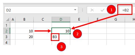
In the above example, if you type (1) =B2 in cell D2, it returns a value of (2) 10. However, typing only (3) B3 into cell D3 just shows “B3” in the cell, and there is no reference to the value 20.
Standard Operators
The next most common symbols in Excel are the standard operators as used on a calculator: plus (+), minus (–), multiply (*) and divide (/). Note that the multiplication sign is not the standard multiplication sign (x) but is depicted by an asterisk (*) while the division sign is not the standard division sign (÷) but is depicted by the forward slash (/).
An example of a formula using addition and multiplication is shown below:
=B1+B2*B3Order of Operations and Adding Parentheses
In the formula shown above, B2*B3 is calculated first, as in standard mathematics. The order of operations is always multiplication before addition. However, you can adjust the order of operations by adding parentheses (round brackets) to the formula; any calculations between these parentheses would then be done first before the multiplication. Parentheses, therefore, are another example of symbols used in Excel.
=(B1+B2)*B3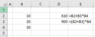
In the example shown above, the first formula returns a value of 610 while the second formula (using parentheses) returns 900.
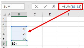
Parentheses are also used with all Excel functions. For example, to sum B3, B4, and B5 together, you can use the SUM Function where the range B3:B5 is contained within parentheses.
=SUM(B3:B5)Colon (:) to Specify a Range of Cells
In the formula used above, the parentheses contain the cell range which the SUM Function needs to add together. This cell range is expressed with a colon (:) where the first cell reference (B3) is the cell address of the first cell included in the range of cells to add together, while the second cell reference (B5) is the cell address of the last cell included in the range.
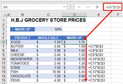
Dollar Symbol ($) in an Absolute Reference
A particular useful and common symbol used in Excel is the dollar sign within a formula. Note that this does not indicate currency; rather, it’s used to “fix” a cell address in place in order that a single cell can be used repetitively in multiple formulas by copying formulas between cells.
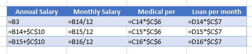
=C6*$C$3By adding a dollar sign ($) in front of the column header (C) and the row header (3), when copying the formula down to Rows 7–15 in the example below, the first part of the formula (e.g., C6) changes according to the row it is copied down to while the second part of the formula ($C$3) stays static always enabling the formula to refer to the value stored in cell C3.
See: Cell References and Absolute Cell Reference Shortcut for more information on absolute references.
Exclamation Point (!) to Indicate a Sheet Name
The exclamation point (!) is critical if you want to create a formula in a sheet and include a reference to a different sheet.
=SUM(Sheet1!B2:B4)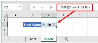
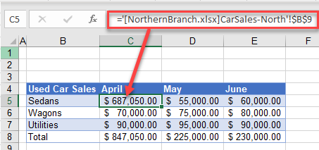
Square Brackets [ ] to Refer to External Workbooks
Excel uses square brackets to show references to linked workbooks. The name of the external workbook is enclosed in square brackets, while the sheet name in that workbook appears after the brackets with an exclamation point at the end.
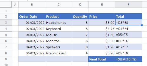
Comma (,)
The comma has two uses in Excel.
Refer to Multiple Ranges
If you wish to use multiple ranges in a function (e.g., the SUM Function), you can use a comma to separate the ranges.
=SUM(B2:B3, B6:B10)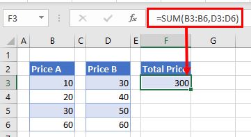
Separate Arguments in a Function
Alternatively, some built in Excel functions have multiple arguments which are usually separated with commas. (These can also be semicolons, depending on the function syntax.)
=VLOOKUP(H5, B6:E15, 4, FALSE)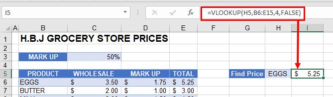
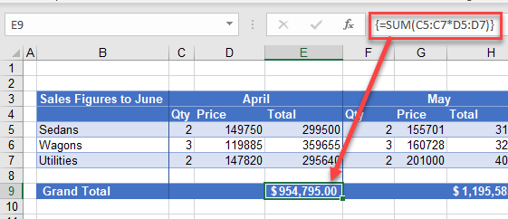
Curly Brackets { } in Array Formulas
Curly brackets are used in array formulas. An array formula is created by pressing the CTRL + SHIFT + ENTER keys together when entering a formula.
Other Important Symbols
| Symbol | Description | Example |
|---|---|---|
| % | Percentage | =B2% |
| ^ | Exponential operator | =B2^B3 |
| & | Concatenation | =B2&B3 |
| > | Greater than | =B2>B3 |
| < | Less than | =B2<B3 |
| >= | Greater than or equal to | =B2>=B3 |
| <= | Less than or equal to | =B2<=B3 |
| <> | Not equal to | =B2<>B3 |
Symbols in Formulas in Google Sheets
The symbols used in Google Sheets are identical to those used in Excel.
If you’re new to Excel for the web, you’ll soon find that it’s more than just a grid in which you enter numbers in columns or rows. Yes, you can use Excel for the web to find totals for a column or row of numbers, but you can also calculate a mortgage payment, solve math or engineering problems, or find a best case scenario based on variable numbers that you plug in.
Excel for the web does this by using formulas in cells. A formula performs calculations or other actions on the data in your worksheet. A formula always starts with an equal sign (=), which can be followed by numbers, math operators (such as a plus or minus sign), and functions, which can really expand the power of a formula.
For example, the following formula multiplies 2 by 3 and then adds 5 to that result to come up with the answer, 11.
=2*3+5
This next formula uses the PMT function to calculate a mortgage payment ($1,073.64), which is based on a 5 percent interest rate (5% divided by 12 months equals the monthly interest rate) over a 30-year period (360 months) for a $200,000 loan:
=PMT(0.05/12,360,200000)
Here are some additional examples of formulas that you can enter in a worksheet.
-
=A1+A2+A3 Adds the values in cells A1, A2, and A3.
-
=SQRT(A1) Uses the SQRT function to return the square root of the value in A1.
-
=TODAY() Returns the current date.
-
=UPPER(«hello») Converts the text «hello» to «HELLO» by using the UPPER worksheet function.
-
=IF(A1>0) Tests the cell A1 to determine if it contains a value greater than 0.
The parts of a formula
A formula can also contain any or all of the following: functions, references, operators, and constants.

1. Functions: The PI() function returns the value of pi: 3.142…
2. References: A2 returns the value in cell A2.
3. Constants: Numbers or text values entered directly into a formula, such as 2.
4. Operators: The ^ (caret) operator raises a number to a power, and the * (asterisk) operator multiplies numbers.
Using constants in formulas
A constant is a value that is not calculated; it always stays the same. For example, the date 10/9/2008, the number 210, and the text «Quarterly Earnings» are all constants. An expression or a value resulting from an expression is not a constant. If you use constants in a formula instead of references to cells (for example, =30+70+110), the result changes only if you modify the formula.
Using calculation operators in formulas
Operators specify the type of calculation that you want to perform on the elements of a formula. There is a default order in which calculations occur (this follows general mathematical rules), but you can change this order by using parentheses.
Types of operators
There are four different types of calculation operators: arithmetic, comparison, text concatenation, and reference.
Arithmetic operators
To perform basic mathematical operations, such as addition, subtraction, multiplication, or division; combine numbers; and produce numeric results, use the following arithmetic operators.
|
Arithmetic operator |
Meaning |
Example |
|
+ (plus sign) |
Addition |
3+3 |
|
– (minus sign) |
Subtraction |
3–1 |
|
* (asterisk) |
Multiplication |
3*3 |
|
/ (forward slash) |
Division |
3/3 |
|
% (percent sign) |
Percent |
20% |
|
^ (caret) |
Exponentiation |
3^2 |
Comparison operators
You can compare two values with the following operators. When two values are compared by using these operators, the result is a logical value — either TRUE or FALSE.
|
Comparison operator |
Meaning |
Example |
|
= (equal sign) |
Equal to |
A1=B1 |
|
> (greater than sign) |
Greater than |
A1>B1 |
|
< (less than sign) |
Less than |
A1<B1 |
|
>= (greater than or equal to sign) |
Greater than or equal to |
A1>=B1 |
|
<= (less than or equal to sign) |
Less than or equal to |
A1<=B1 |
|
<> (not equal to sign) |
Not equal to |
A1<>B1 |
Text concatenation operator
Use the ampersand (&) to concatenate (join) one or more text strings to produce a single piece of text.
|
Text operator |
Meaning |
Example |
|
& (ampersand) |
Connects, or concatenates, two values to produce one continuous text value |
«North»&»wind» results in «Northwind» |
Reference operators
Combine ranges of cells for calculations with the following operators.
|
Reference operator |
Meaning |
Example |
|
: (colon) |
Range operator, which produces one reference to all the cells between two references, including the two references. |
B5:B15 |
|
, (comma) |
Union operator, which combines multiple references into one reference |
SUM(B5:B15,D5:D15) |
|
(space) |
Intersection operator, which produces one reference to cells common to the two references |
B7:D7 C6:C8 |
The order in which Excel for the web performs operations in formulas
In some cases, the order in which a calculation is performed can affect the return value of the formula, so it’s important to understand how the order is determined and how you can change the order to obtain the results you want.
Calculation order
Formulas calculate values in a specific order. A formula always begins with an equal sign (=). Excel for the web interprets the characters that follow the equal sign as a formula. Following the equal sign are the elements to be calculated (the operands), such as constants or cell references. These are separated by calculation operators. Excel for the web calculates the formula from left to right, according to a specific order for each operator in the formula.
Operator precedence
If you combine several operators in a single formula, Excel for the web performs the operations in the order shown in the following table. If a formula contains operators with the same precedence—for example, if a formula contains both a multiplication and division operator— Excel for the web evaluates the operators from left to right.
|
Operator |
Description |
|
: (colon) (single space) , (comma) |
Reference operators |
|
– |
Negation (as in –1) |
|
% |
Percent |
|
^ |
Exponentiation |
|
* and / |
Multiplication and division |
|
+ and – |
Addition and subtraction |
|
& |
Connects two strings of text (concatenation) |
|
= |
Comparison |
Use of parentheses
To change the order of evaluation, enclose in parentheses the part of the formula to be calculated first. For example, the following formula produces 11 because Excel for the web performs multiplication before addition. The formula multiplies 2 by 3 and then adds 5 to the result.
=5+2*3
In contrast, if you use parentheses to change the syntax, Excel for the web adds 5 and 2 together and then multiplies the result by 3 to produce 21.
=(5+2)*3
In the following example, the parentheses that enclose the first part of the formula force Excel for the web to calculate B4+25 first and then divide the result by the sum of the values in cells D5, E5, and F5.
=(B4+25)/SUM(D5:F5)
Using functions and nested functions in formulas
Functions are predefined formulas that perform calculations by using specific values, called arguments, in a particular order, or structure. Functions can be used to perform simple or complex calculations.
The syntax of functions
The following example of the ROUND function rounding off a number in cell A10 illustrates the syntax of a function.
1. Structure. The structure of a function begins with an equal sign (=), followed by the function name, an opening parenthesis, the arguments for the function separated by commas, and a closing parenthesis.
2. Function name. For a list of available functions, click a cell and press SHIFT+F3.
3. Arguments. Arguments can be numbers, text, logical values such as TRUE or FALSE, arrays, error values such as #N/A, or cell references. The argument you designate must produce a valid value for that argument. Arguments can also be constants, formulas, or other functions.
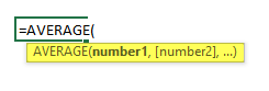
4. Argument tooltip. A tooltip with the syntax and arguments appears as you type the function. For example, type =ROUND( and the tooltip appears. Tooltips appear only for built-in functions.
Entering functions
When you create a formula that contains a function, you can use the Insert Function dialog box to help you enter worksheet functions. As you enter a function into the formula, the Insert Function dialog box displays the name of the function, each of its arguments, a description of the function and each argument, the current result of the function, and the current result of the entire formula.
To make it easier to create and edit formulas and minimize typing and syntax errors, use Formula AutoComplete. After you type an = (equal sign) and beginning letters or a display trigger, Excel for the web displays, below the cell, a dynamic drop-down list of valid functions, arguments, and names that match the letters or trigger. You can then insert an item from the drop-down list into the formula.
Nesting functions
In certain cases, you may need to use a function as one of the arguments of another function. For example, the following formula uses a nested AVERAGE function and compares the result with the value 50.
1. The AVERAGE and SUM functions are nested within the IF function.
Valid returns When a nested function is used as an argument, the nested function must return the same type of value that the argument uses. For example, if the argument returns a TRUE or FALSE value, the nested function must return a TRUE or FALSE value. If the function doesn’t, Excel for the web displays a #VALUE! error value.
Nesting level limits A formula can contain up to seven levels of nested functions. When one function (we’ll call this Function B) is used as an argument in another function (we’ll call this Function A), Function B acts as a second-level function. For example, the AVERAGE function and the SUM function are both second-level functions if they are used as arguments of the IF function. A function nested within the nested AVERAGE function is then a third-level function, and so on.
Using references in formulas
A reference identifies a cell or a range of cells on a worksheet, and tells Excel for the web where to look for the values or data you want to use in a formula. You can use references to use data contained in different parts of a worksheet in one formula or use the value from one cell in several formulas. You can also refer to cells on other sheets in the same workbook, and to other workbooks. References to cells in other workbooks are called links or external references.
The A1 reference style
The default reference style By default, Excel for the web uses the A1 reference style, which refers to columns with letters (A through XFD, for a total of 16,384 columns) and refers to rows with numbers (1 through 1,048,576). These letters and numbers are called row and column headings. To refer to a cell, enter the column letter followed by the row number. For example, B2 refers to the cell at the intersection of column B and row 2.
|
To refer to |
Use |
|
The cell in column A and row 10 |
A10 |
|
The range of cells in column A and rows 10 through 20 |
A10:A20 |
|
The range of cells in row 15 and columns B through E |
B15:E15 |
|
All cells in row 5 |
5:5 |
|
All cells in rows 5 through 10 |
5:10 |
|
All cells in column H |
H:H |
|
All cells in columns H through J |
H:J |
|
The range of cells in columns A through E and rows 10 through 20 |
A10:E20 |
Making a reference to another worksheet In the following example, the AVERAGE worksheet function calculates the average value for the range B1:B10 on the worksheet named Marketing in the same workbook.

1. Refers to the worksheet named Marketing
2. Refers to the range of cells between B1 and B10, inclusively
3. Separates the worksheet reference from the cell range reference
The difference between absolute, relative and mixed references
Relative references A relative cell reference in a formula, such as A1, is based on the relative position of the cell that contains the formula and the cell the reference refers to. If the position of the cell that contains the formula changes, the reference is changed. If you copy or fill the formula across rows or down columns, the reference automatically adjusts. By default, new formulas use relative references. For example, if you copy or fill a relative reference in cell B2 to cell B3, it automatically adjusts from =A1 to =A2.

Absolute references An absolute cell reference in a formula, such as $A$1, always refer to a cell in a specific location. If the position of the cell that contains the formula changes, the absolute reference remains the same. If you copy or fill the formula across rows or down columns, the absolute reference does not adjust. By default, new formulas use relative references, so you may need to switch them to absolute references. For example, if you copy or fill an absolute reference in cell B2 to cell B3, it stays the same in both cells: =$A$1.

Mixed references A mixed reference has either an absolute column and relative row, or absolute row and relative column. An absolute column reference takes the form $A1, $B1, and so on. An absolute row reference takes the form A$1, B$1, and so on. If the position of the cell that contains the formula changes, the relative reference is changed, and the absolute reference does not change. If you copy or fill the formula across rows or down columns, the relative reference automatically adjusts, and the absolute reference does not adjust. For example, if you copy or fill a mixed reference from cell A2 to B3, it adjusts from =A$1 to =B$1.

The 3-D reference style
Conveniently referencing multiple worksheets If you want to analyze data in the same cell or range of cells on multiple worksheets within a workbook, use a 3-D reference. A 3-D reference includes the cell or range reference, preceded by a range of worksheet names. Excel for the web uses any worksheets stored between the starting and ending names of the reference. For example, =SUM(Sheet2:Sheet13!B5) adds all the values contained in cell B5 on all the worksheets between and including Sheet 2 and Sheet 13.
-
You can use 3-D references to refer to cells on other sheets, to define names, and to create formulas by using the following functions: SUM, AVERAGE, AVERAGEA, COUNT, COUNTA, MAX, MAXA, MIN, MINA, PRODUCT, STDEV.P, STDEV.S, STDEVA, STDEVPA, VAR.P, VAR.S, VARA, and VARPA.
-
3-D references cannot be used in array formulas.
-
3-D references cannot be used with the intersection operator (a single space) or in formulas that use implicit intersection.
What occurs when you move, copy, insert, or delete worksheets The following examples explain what happens when you move, copy, insert, or delete worksheets that are included in a 3-D reference. The examples use the formula =SUM(Sheet2:Sheet6!A2:A5) to add cells A2 through A5 on worksheets 2 through 6.
-
Insert or copy If you insert or copy sheets between Sheet2 and Sheet6 (the endpoints in this example), Excel for the web includes all values in cells A2 through A5 from the added sheets in the calculations.
-
Delete If you delete sheets between Sheet2 and Sheet6, Excel for the web removes their values from the calculation.
-
Move If you move sheets from between Sheet2 and Sheet6 to a location outside the referenced sheet range, Excel for the web removes their values from the calculation.
-
Move an endpoint If you move Sheet2 or Sheet6 to another location in the same workbook, Excel for the web adjusts the calculation to accommodate the new range of sheets between them.
-
Delete an endpoint If you delete Sheet2 or Sheet6, Excel for the web adjusts the calculation to accommodate the range of sheets between them.
The R1C1 reference style
You can also use a reference style where both the rows and the columns on the worksheet are numbered. The R1C1 reference style is useful for computing row and column positions in macros. In the R1C1 style, Excel for the web indicates the location of a cell with an «R» followed by a row number and a «C» followed by a column number.
|
Reference |
Meaning |
|
R[-2]C |
A relative reference to the cell two rows up and in the same column |
|
R[2]C[2] |
A relative reference to the cell two rows down and two columns to the right |
|
R2C2 |
An absolute reference to the cell in the second row and in the second column |
|
R[-1] |
A relative reference to the entire row above the active cell |
|
R |
An absolute reference to the current row |
When you record a macro, Excel for the web records some commands by using the R1C1 reference style. For example, if you record a command, such as clicking the AutoSum button to insert a formula that adds a range of cells, Excel for the web records the formula by using R1C1 style, not A1 style, references.
Using names in formulas
You can create defined names to represent cells, ranges of cells, formulas, constants, or Excel for the web tables. A name is a meaningful shorthand that makes it easier to understand the purpose of a cell reference, constant, formula, or table, each of which may be difficult to comprehend at first glance. The following information shows common examples of names and how using them in formulas can improve clarity and make formulas easier to understand.
|
Example Type |
Example, using ranges instead of names |
Example, using names |
|
Reference |
=SUM(A16:A20) |
=SUM(Sales) |
|
Constant |
=PRODUCT(A12,9.5%) |
=PRODUCT(Price,KCTaxRate) |
|
Formula |
=TEXT(VLOOKUP(MAX(A16,A20),A16:B20,2,FALSE),»m/dd/yyyy») |
=TEXT(VLOOKUP(MAX(Sales),SalesInfo,2,FALSE),»m/dd/yyyy») |
|
Table |
A22:B25 |
=PRODUCT(Price,Table1[@Tax Rate]) |
Types of names
There are several types of names that you can create and use.
Defined name A name that represents a cell, range of cells, formula, or constant value. You can create your own defined name. Also, Excel for the web sometimes creates a defined name for you, such as when you set a print area.
Table name A name for an Excel for the web table, which is a collection of data about a particular subject that is stored in records (rows) and fields (columns). Excel for the web creates a default Excel for the web table name of «Table1», «Table2», and so on, each time you insert an Excel for the web table, but you can change these names to make them more meaningful.
Creating and entering names
You create a name by using Create a name from selection. You can conveniently create names from existing row and column labels by using a selection of cells in the worksheet.
Note: By default, names use absolute cell references.
You can enter a name by:
-
Typing Typing the name, for example, as an argument to a formula.
-
Using Formula AutoComplete Use the Formula AutoComplete drop-down list, where valid names are automatically listed for you.
Using array formulas and array constants
Excel for the web doesn’t support creating array formulas. You can view the results of array formulas created in Excel desktop application, but you can’t edit or recalculate them. If you have the Excel desktop application, click Open in Excel to work with arrays.
The following array example calculates the total value of an array of stock prices and shares, without using a row of cells to calculate and display the individual values for each stock.
When you enter the formula ={SUM(B2:D2*B3:D3)} as an array formula, it multiples the Shares and Price for each stock, and then adds the results of those calculations together.
To calculate multiple results Some worksheet functions return arrays of values, or require an array of values as an argument. To calculate multiple results with an array formula, you must enter the array into a range of cells that has the same number of rows and columns as the array arguments.
For example, given a series of three sales figures (in column B) for a series of three months (in column A), the TREND function determines the straight-line values for the sales figures. To display all the results of the formula, it is entered into three cells in column C (C1:C3).
When you enter the formula =TREND(B1:B3,A1:A3) as an array formula, it produces three separate results (22196, 17079, and 11962), based on the three sales figures and the three months.
Using array constants
In an ordinary formula, you can enter a reference to a cell containing a value, or the value itself, also called a constant. Similarly, in an array formula you can enter a reference to an array, or enter the array of values contained within the cells, also called an array constant. Array formulas accept constants in the same way that non-array formulas do, but you must enter the array constants in a certain format.
Array constants can contain numbers, text, logical values such as TRUE or FALSE, or error values such as #N/A. Different types of values can be in the same array constant — for example, {1,3,4;TRUE,FALSE,TRUE}. Numbers in array constants can be in integer, decimal, or scientific format. Text must be enclosed in double quotation marks — for example, «Tuesday».
Array constants cannot contain cell references, columns or rows of unequal length, formulas, or the special characters $ (dollar sign), parentheses, or % (percent sign).
When you format array constants, make sure you:
-
Enclose them in braces ( { } ).
-
Separate values in different columns by using commas (,). For example, to represent the values 10, 20, 30, and 40, you enter {10,20,30,40}. This array constant is known as a 1-by-4 array and is equivalent to a 1-row-by-4-column reference.
-
Separate values in different rows by using semicolons (;). For example, to represent the values 10, 20, 30, and 40 in one row and 50, 60, 70, and 80 in the row immediately below, you enter a 2-by-4 array constant: {10,20,30,40;50,60,70,80}.
![]()
Symbols Used in Excel Formula

Here are the important symbols used in Excel Formulas. Each of these special characters have used for different purpose in Excel. Let us see complete list of symbols used in Excel Formulas, its meaning and uses.
Symbols used in Excel Formula
Following symbols are used in Excel Formula. They will perform different actions in Excel Formulas and Functions.
| Symbol | Name | Description |
|---|---|---|
| = | Equal to | Every Excel Formula begins with Equal to symbol (=).
Example:=A1+A5 |
| () | Parentheses | All Arguments of the Excel Functions specified between the Parentheses.
Example:=COUNTIF(A1:A5,5) |
| () | Parentheses | Expressions specified in the Parentheses will be evaluated first. Parentheses changes the order of the evaluation in Excel Formula.
Example: =25+(35*2)+5 |
| * | Asterisk | Wild card operator to to denote all values in a List.
Example: =COUNTIF(A1:A5,”*“) |
| , | Comma | List of the Arguments of a Function Separated by Comma in Excel Formula.
Example: =COUNTIF(A1:A5,“>” &B1) |
| & | Ampersand | Concatenate Operator to connect two strings into one in Excel Formula.
Example: =”Total: “&SUM(B2:B25) |
| $ | Dollar | Makes Cell Reference as Absolute in Excel Formula.
Example:=SUM($B$2:$B$25) |
| ! | Exclamation | Sheet Names and Table Names Followed by ! Symbol in Excel Formula.
Example: =SUM(Sheet2!B2:B25) |
| [] | Square Brackets | Uses to refer the Field Name of the Table (List Object) in Excel Formula.
Example:=SUM(Table1[Column1]) |
| {} | Curly Brackets | Denote the Array formula in Excel.
Example: {=MAX(A1:A5-G1:G5)} |
| : | Colon | Creates references to all cells between two references.
Example: =SUM(B2:B25) |
| , | Comma | Union Operator will combine the multiple references into One.
Example: =SUM(A2:A25, B2:B25) |
| (space) | Space | Intersection Operator will create common reference of two references.
Example: =SUM(A2:A10 A5:A25) |
Share This Story, Choose Your Platform!
6 Comments
-
Redjen
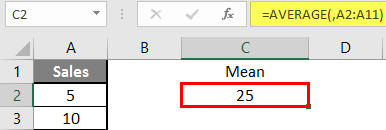
May 31, 2022 at 12:37 pm — Replywhat is the symbol of average in excel?
-
PNRao
June 20, 2022 at 12:40 pm — ReplyYou can use AVERAGE()Function to calculate Average in Excel. If you wants to show the Average Statistical Symbol (x-bar), You can insert from symbols. F7C2 is the Unicode Hexa character for X-bar symbol. Make sure that you have set the Symbol Font :MS Reference Sans Serif.
-
-
Tom Pearce
September 22, 2022 at 3:54 pm — ReplyI have a workbook, where the original author used an @ sign in front of a function call in a formula. I can find no reference as to what the @ does, or how it is used. Any one know??
VBA Example: ActiveSheet.Range(“L2”).Formula = “=@CATEGORY($E2,LFC_AreaLU)”
Note: Category is a User Defined Function in the workbook.-
PNRao
December 5, 2022 at 11:30 am — Reply
-
-
Jane Girard
February 9, 2023 at 8:53 pm — ReplyI have this formula, do you know what the al means in the formula ?
IF(E4=””,””,VLOOKUP(C4,al,5,0)*E4), can-
PNRao
February 27, 2023 at 3:10 am — ReplyIt could be a defined Name or a name of the Table (List Object)
-
© Copyright 2012 – 2020 | Excelx.com | All Rights Reserved
Page load link
15 Most Common Excel Functions You Must Know + How to Use Them
Microsoft Excel is one of the most well-known computer applications. It has changed the way people and companies work with data.
Thus, learning Excel can help with both your career and your personal needs.
Excel runs using functions and there are roughly 500 of them! These range from basic arithmetic to complex statistics.

If you’re a new Excel user, this sheer quantity can be quite daunting.
So we are here to help you! 🤝
We have rounded up 15 of the most common and useful Excel functions that you need to learn. We also prepared a practice workbook for you to follow along with the examples. Download it here.
Let’s get started!
What are Excel functions?
Excel is used to calculate and manipulate numbers and text. To do this, you use formulas!
Formulas are expressions that tell Excel what you want to do with the data. They begin with the equal symbol (=) followed by a combination of operators and functions.
What are operators?
These are symbols that specify the type of calculation you want to perform on the elements of a formula.
For example, to add two numbers, you can type “=1+1” into a cell. Once you hit Enter, Excel will run the formula and return the result which is 2.
Here are some examples of common operators:

Excel automatically treats cell contents that start with (=) as formulas. This also applies when you begin a cell with the plus (+) or minus (-) symbols.
You can bypass this by adding a leading apostrophe (‘). This is how you can show formulas as text like in the table above.
Order of operation and using parentheses in Excel formulas
Generally, Excel follows PEMDAS when calculating formulas. PEMDAS means parentheses first, then exponents, then multiplication and division, then addition and subtraction.

What are functions?
These are predefined processes in Excel. Each function in Excel has a unique name and specific input(s). The function takes these inputs and performs the corresponding calculation.
The inputs or arguments of an Excel function are always enclosed in parentheses.
For example, this is the syntax for the MAX function:
=MAX(number1, [number2], …)
The list of numbers where you want to find the maximum value is placed inside the parentheses.

Using a cell or a range as input
As you learn more about Excel, you’ll find that Excel formulas rarely consist of individual numbers only like in the formula “=1+1”.

Thus, referencing cells is important in Excel and you can learn more by clicking here.
Alright! You’ve just learned how a function in Excel works.
Let’s dive right into the list! 🤿
We will start with basic Excel functions and then move on to more advanced functions.
Basic Math Functions (Beginner Level ★☆☆)
1. SUM
This is the first function in Excel that most new users need. As the name implies, the SUM function adds up all the values in a specified group of cells or range.
Syntax: =SUM(number1, [number2], …)
Try it out in the practice workbook.

If you want to get the total quiz score for each student, you can use the SUM function. In this case, the input range will be all four quiz scores for each student.
1. Type this formula into cell F2:
=SUM(B2:E2)
You can also type “=SUM(B2,C2,D2,E2)” but “=SUM(B2:E2)” is much simpler.

2. Press Enter. Excel then evaluates the formula and the cell returns the number for the total which is 360.
3. Copy this for the rest of the students or drag down the fill handle.

Notice that the SUM function ignores the cells containing text. (“X” meaning the student was unable to take the quiz)
Most of the basic math functions in Excel ignore non-numeric values such as text, date, and time.
2. COUNT
Next up is the COUNT function. It returns the number of cells containing numeric values within the input range.
Syntax: =COUNT(value1, [value2], …)
1. To get the number of quizzes taken by each student, use this formula in cell G2:
=COUNT(B2:E2)
2. Hit Enter and fill in the rows below.

If you would like to include non-numeric values in the count, you can use the COUNTA function. To count the number of blank cells, you can use the COUNTBLANK function.
Learn more about the COUNT function and its variants here.
3. AVERAGE
The average of a list of numbers is just the total divided by how many numbers there are in that list.
This is easy enough to calculate the quiz scores. You already have the SUM and the COUNT of quizzes for each student.
But, it gets even easier using the AVERAGE function in Excel.
Syntax: =AVERAGE (value1, [value2], …)
1. Type this into cell H2:
=AVERAGE(B2:E2)
2. Hit Enter and fill in the rows below.


Logical Functions (Intermediate Level – ★★☆)
Let’s raise the difficulty level a little bit.
A logical function in Excel allows you to make comparisons and use the results to change how a formula calculates.
4. IF
The IF function is a very popular function in Excel and it is actually quite easy to learn.
Syntax: =IF(logical_test, value_if_true, [value_if_false])
This function checks if a logical test is either TRUE or FALSE. It then returns the specified value based on the result.

Using the average score of each student, try to assign PASS or FAIL grades. Assume that the passing score for this class is 60.
1. Begin the formula in cell C2 with “=IF(“
The logical_test is to check if the average score in Column B is greater than or equal to (>=) the passing score of 60.
2. So, the formula becomes:
=IF(B2>=60,
If the comparison returns TRUE, then the formula should return the text “PASS”. Thus, the value_if_true argument should be “PASS”.
And if it returns FALSE, then the value_if_false argument should be “FAIL”.
3. Thus, the formula becomes:
=IF(B2>=60,”PASS”,”FAIL”)
4. Hit Enter and fill in the rows below.

What if you needed to assign grades according to a scale instead of just “PASS” and “FAIL”?
For that, you have to use multiple criteria or logical tests. While this is possible using nested IF functions, it can get messy very quickly. Instead, you can use the IFS function.
5. IFS function
The IFS function was introduced in Excel 2016 to replace nested IF functions.
This function works by evaluating the first logical test or criteria. It returns the corresponding value if it is TRUE. But if it is FALSE, the function proceeds to evaluate the second criteria, and so on.
📖 In other words, the IFS function outputs the value that corresponds to the first specified criteria that is true.
Syntax: =IFS(logical_test1, value_if_true1, [logical_test2], [value_if_true2],..)

1. First, the formula should check if the average score (column B) is above or equal to 90. If yes, it should return “A”.
=IFS(B2>=90,”A”,
2. If not, it should then check if the average score is greater than or equal to 80. If yes, it should return “B”. If you do this up to grade D, the formula becomes:
=IFS(B2>=90,”A”,B2>=80,”B”,B2>=70,”C”,B2>=60,”D”,
3. For the last grade “F”, put “TRUE” for the logical test.
The IFS function will only evaluate the last specified criteria if all of the previous logical values were FALSE. Thus, you can set the last criteria to always be TRUE thus making it a “catch all” statement.
The final formula is then:
=IFS(B2>=90,”A”,B2>=80,”B”,B2>=70,”C”,B2>=60,”D”,TRUE,”F”)

PRO-TIP:
You can use absolute cell references and a reference table when working with long formulas.
That way, you don’t have to revisit all of the arguments in the formula if you need to change some values.
For example, using the table and formula shown below, you can easily change the grading scale in use.
=IFS(B2>=$H$2,$F$2,B2>=$H$3,$F$3,B2>
=$H$4,$F$4,B2>=$H$5,$F$5,TRUE,$F$6)

Text Functions (Intermediate Level – ★★☆)
In this next section, you will see how Excel can also be used to manipulate text.
In the “Class List” worksheet of the practice workbook, the full name of each student is listed in Column A. Your goal is to rearrange these from “first name last name” to “last name_first name” in Column F.

To do this, you first have to extract the first name and the last name from Column A.
6. FIND
The names are separated by a space character ” “. So, you have to identify the position of the space within each text string in Column A.
The FIND function in Excel returns the number or position of a specified character or substring within another text string.
Syntax: =FIND(find_text, within_text, [start_num])
To get the position of the space ” “, type this formula:
=FIND(” “,A2)

Next, take a look at the LEN function.
7. LEN
This function returns the number of characters in a text string.
Syntax: =LEN(text)
To get the number of characters in each student’s name:
=LEN(A2)

Now you can move on to extracting the first and last name using the MID function in Excel.
8. MID
This function extracts a given number of characters from the middle of a text string.
Syntax: = MID(text, start_num, num_chars)
It is one of three text functions that are used to extract text. The other two are LEFT and RIGHT which extract text from the start and end of a text string respectively.
The first name starts at the very first character of the text string. So, you extract starting from position 1. Then the length of the first name is given by the position of the space character minus 1.
So, the formula to extract the first name or first word from a text string is:
=MID(A2,1,B2-1)
Or, you can express it directly using the FIND formula earlier.
=MID(A2,1,FIND(” “,A2)-1)

For the last name, you can extract it starting from the position of the space character plus 1. Its length is just the length of the entire text string minus the position of the space character.
=MID(A2,B2+1,C2-B2)
Or, using the FIND and LEN formulas earlier:
=MID(A2,FIND(” “,A2)+1,LEN(A2)-FIND(” “,A2))

Now you can combine the last name and the first name in the desired order using the CONCAT function.
9. CONCAT
Like IFS, CONCAT is another newly introduced function in Excel 2016. It replaced the old CONCATENATE function.
Syntax: =CONCAT(text1, [text2],…)
Combine the last name and the first name with a comma and space character “, ” in between.
=CONCAT(E2,”, “,D2)

PRO-TIP:
In the above example, you used helper columns for FIND, LEN, and MID to help build the final formula and visualize how it works.
In real-world applications, you can use a single long formula to get the results like this:
=CONCAT(MID(A2,FIND(” “,A2)+1,LEN(A2)
-FIND(” “,A2)),”, “,MID(A2,1,FIND(” “,A2)-1))

Lookup and Reference Functions (Advanced Level – ★★★)
In this final section, we will focus on functions that allow you to look for specific data points and refer to them.
Take a look at the “Schedule” worksheet.

10. COLUMN
The COLUMN function in Excel returns the column number of a given cell.
Syntax: =COLUMN([reference])
Let’s try to assign specific dates for each quiz. For example, you may want the quizzes to be held every Monday. This means that the first quiz date should be offset by 1 week or 7 days for each succeeding quiz date.
You can use the column number to multiply the 7 days offset for each week like this:
=$B$2+(COLUMN()-2)*7

Two (2) is subtracted from the column number so that the sequence starts at 1.
You can also get this result using the much simpler “=B2+7” since you are only adding a fixed number of days to each date. 🤔
But, using the COLUMN function, you can create complex patterns.
Take this pattern for example:
The quizzes are still held every Monday. But every third week, they are held on Wednesday instead.
Here is the formula for this pattern:
=$B$2+(COLUMN()-2)*7+IF(MOD(COLUMN()-1,3)=0,2,0)


The MOD function in Excel returns the remainder after a number is divided by a given divisor. It’s part of the Math & Trig group of functions.
This group includes other fun functions such as ABS which returns the absolute value of a number and ROUND which rounds a number to a specified number of digits.
Learn more about the function groups towards the end of this article!
11. ROW
Next, take a look at the ROW function. It works exactly like COLUMN but it returns the row number instead.
Syntax: =ROW([reference])
In this next example, you will assign the seating plans. You can try different seating arrangements using the ROW function.
Assume R1C1 is the seat closest to the teacher’s desk.
1. You can have the students seated one seat after another and in two columns:
=CONCAT(“R”,MOD(ROW()-6,3)*2+1,”C”,INT((ROW()-6)/3)*2+1)

2. Or they can sit in rows of 3 and columns of 2
=CONCAT(“R”,MOD(ROW()-6,2)*2+1,”C”,INT((ROW()-6)/2)*2+1)

3. You can also sit them in the farthest rows:
=CONCAT(“R”,MOD(ROW()-6,2)*4+1,”C”,INT((ROW()-6)/2)*2+1)

4. Or in the farthest columns:
=CONCAT(“R”,MOD(ROW()-6,3)*2+1,”C”,INT((ROW()-6)/3)*4+1)

Manually creating seating patterns for small sets like this one is easy. But a formula like those shown above definitely helps especially for larger sets like 50, 100, or even more.
The COLUMN and ROW functions are rarely used on their own. Like IF and IFS, you use them with other functions to change how the formula is calculated.
12. MATCH
Now, open up the “Lookup” worksheet.
In the next few examples, you will create a search feature that allows students to look up their names. They can then see their scores from past quizzes and their assigned seats for the next quizzes.
To start, you will use the MATCH function. It searches for a specified item within a given range of cells. It then returns the relative position of the first match.
Syntax: =MATCH(lookup_value, lookup_array, [match_type])
- The lookup_value is the item you want to search for. So, set this to cell B2.
- The lookup_array is the range or table array where you want to search. Use F2:F7 from the “Class List” worksheet.
- For the match_type, set this to zero so that the function searches for an exact match. (Learn more about MATCH and the different match types in this article)
The formula then becomes:
=MATCH(B2,’Class List’!F2:F7,0)

However, it only works correctly if the name is entered exactly as it is written in Column F of the Class List.
To fix this, you can use the asterisk “*” wildcard character so that searching for either first or last name works.
You can also enclose the formula in an IFNA function. This way, if the formula cannot find the given name in the table, it will return a phrase like “No result found”.


13. INDEX
The INDEX function retrieves a value from a given table array based on the provided row and column numbers.
Syntax: =INDEX (array, row_num, [col_num])
Similar to the MATCH example, you need to specify where the range or array lookup is.

For row_num, you can use the earlier MATCH result at Cell B5. Then for col_num, use 1 for the First Name:
=INDEX(‘Class List’!D2:E7,B5,1)

And set col_num to 2 for the Last Name.
=INDEX(‘Class List’!D2:E7,B5,2)

Just like that, you have a working search 🔍 formula!
This is just a small example of the countless possibilities using the INDEX and MATCH combination. Click here for more examples!
14. VLOOKUP
The VLOOKUP function in Excel works similarly to the INDEX and MATCH combination. It is faster to set up but it is less versatile. VLOOKUP also only works if your lookup array is at the leftmost of the reference table.
Syntax: =VLOOKUP (lookup_value, table_array, col_index_num, [range_lookup])
This time, you will use the First Name result (cell B6) as the lookup_value. Use this and VLOOKUP to retrieve the given student’s scores from the “Quiz Scores” worksheet.
=VLOOKUP($B$6,’Quiz Scores’!$A$2:$E$7,COLUMN(),FALSE)

For the seat assignment, use the Last Name result followed by the asterisk wild character.
=VLOOKUP($B$7&”*”,Schedule!$A$6:$E$11,COLUMN(),FALSE)

15. INDIRECT
The last function that you will be learning about today is also one of the most powerful in Excel.
INDIRECT allows you to specify cell references using text strings.
SYNTAX: =INDIRECT(ref_text, [a1])
For example, instead of typing “=A1”, you can type “=INDIRECT(“A”&1). This means you can dynamically change references.
Let’s take the INDEX & MATCH formula you used to retrieve the Last Name. You can get the same result using this formula:
=INDIRECT(“‘Class List’!”&”E”&(B5+1))

The INDIRECT function opens up so many possibilities with dynamic references in Excel. I highly this article for an in-depth tutorial on INDIRECT.
That’s it – Now what?
As you have just learned, Excel offers so many different functions to choose from. Luckily, Excel has brought them all together in the Formulas tab.

You can look for an Excel function using search keywords or you can also select from the categorical dropdowns.
For example, click on the Financial group to find functions that can help you calculate items like net present value, future value, cumulative interest paid, cumulative principal paid, etc.

You can also click on More Functions which opens up even more possibilities for advanced Excel formulas.
For example, the Statistical group is useful if you need to calculate a statistical value. This includes functions for maximum value, minimum value, forecast value, gamma function value, etc. You can insert a cumulative distribution function and other useful tools for data analysis.

Learn how to use these formulas and more by signing up for my free online Excel course.
We will help you make the most out of your Excel experience! 📈
Other relevant resources
If you enjoyed this article, you can visit my YouTube channel for more in-depth tutorials and other fun stuff!
Did you know that the Flash Fill feature can help speed up your work by automatically filling a repetitive pattern Excel detects from your data? Learn more here.
Thanks for reading! 😄
Kasper Langmann2023-02-23T11:47:15+00:00
Page load link
How to Find Mean in Excel (Table of Content)
- Introduction to Mean in Excel
- Example of Mean in Excel
Introduction to Mean in Excel
The average function is used to calculate the Arithmetic Mean of the given input. It is used to do sum of all arguments and divide it by the count of arguments where the half set of the number will be smaller than the mean, and the remaining set will be greater than the mean. It will return the arithmetic mean of the number based on provided input. It is an in-built Statistical function. A user can give 255 input arguments in the function.
As an example, suppose there is 4 number 5,10,15,20 if a user wants to calculate the mean of the numbers then it will return 12.5 as the result of =AVERAGE (5, 10, 15, 20).
The formula of Mean: It is used to return the mean of the provided number where a half set of the number will be smaller than the number, and the remaining set will be greater than the mean.
The argument of the Function:
- number1: It is a mandatory argument in which functions will take to calculate the mean.
- [number2]: It is an optional argument in the function.
Examples on How to Find Mean in Excel
Here are some examples of how to find mean in excel with the steps and the calculation
You can download this How to Find Mean Excel Template here – How to Find Mean Excel Template
Example #1 – How to Calculate the Basic Mean in Excel
Let’s assume there is a user who wants to perform the calculation for all numbers in Excel. Let’s see how we can do this with the average function.
Step 1: Open MS Excel from the start menu >> Go to Sheet1, where the user has kept the data.
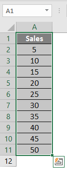
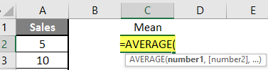
Step 2: Now create headers for Mean where we will calculate the mean of the numbers.
![]()
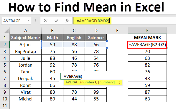
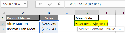
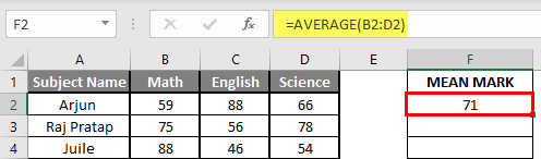
Step 3: Now calculate the mean of the given number by average function>> use the equal sign to calculate >> Write in cell C2 and use average>> “=AVERAGE (“
Step 3: Now, it will ask for a number1, which is given in column A >> there are 2 methods to provide input either a user can give one by one or just give the range of data >> select data set from A2 to A11 >> write in cell C2 and use average>> “=AVERAGE (A2: A11) “
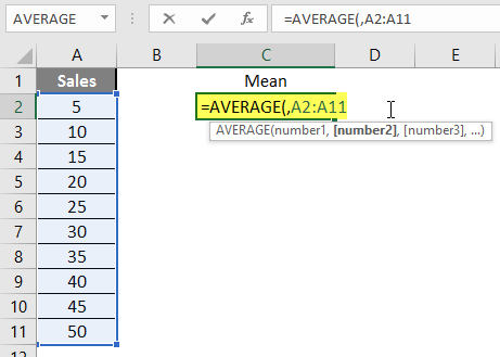
Step 4: Now press the enter key >> Mean will be calculated.
Summary of Example 1: As the user wants to perform the mean calculation for all numbers in MS Excel. Easley everything calculated in the above excel example, and the Mean is 27.5 for sales.
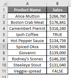
Example #2 – How to Calculate Mean if Text Value Exists in the Data Set
Let’s calculate the Mean if there is some text value in the Excel data set. Let’s assume a user wants to perform the calculation for some sales data set in Excel. But there is some text value also there. So, he wants to use count for all, either its text or number. Let’s see how we can do this with the AVERAGE function. Because in the normal AVERAGE function, it will exclude the text value count.
Step 1: Open MS Excel from the start menu >> Go to Sheet2, where the user has kept the data.
Step 2: Now create headers for Mean where we will calculate the mean of the numbers.
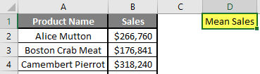
Step 3: Now calculate the mean of the given number by average function>> use the equal sign to calculate >> Write in cell D2 and use AVERAGEA>> “=AVERAGEA (“
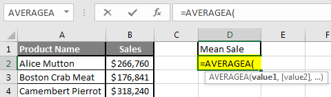
Step 4: Now, it will ask for a number1, which is given in column B >> there is two open to provide input either a user can give one by one or just give the range of data >> select data set from B2 to B11 >> write in D2 Cell and use average>> “=AVERAGEA (D2: D11) “
Step 5: Now click on the enter button >> Mean will be calculated.
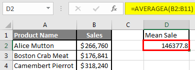
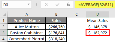
Step 6: Just to compare the AVERAGEA and AVERAGE, in normal average, it will exclude the count for text value so mean will high than the AVERAGE MEAN.
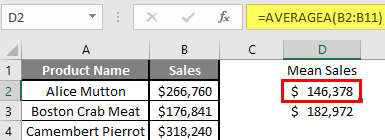
Summary of Example 2: As the user wants to perform the mean calculation for all number in MS Excel. Easley, everything calculated in the above excel example and the Mean is $146377.80 for sales.
Example #3 – How to Calculate Mean for Different Set of Data
Let’s assume a user wants to perform the calculation for some student’s mark data set in MS Excel. There are ten student marks for Math, English, and Science out of 100. Let’s see How to Find Mean in Excel with the AVERAGE function.
Step 1: Open the MS Excel from the start menu >> Go to Sheet3, where the user kept the data.
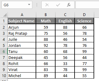
Step 2: Now create headers for Mean where we will calculate the mean of the numbers.
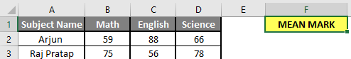
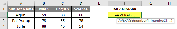
Step 3: Now calculate the mean of the given number by average function>> use the equal sign to calculate >> Write in F2 Cell and use AVERAGE >> “=AVERAGE (“
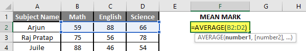
Step 3: Now, it will ask for number1 which is given in B, C, and D column >> there is two open to provide input either a user can give one by one or just give the range of data >> Select data set from B2 to D2 >> Write in F2 Cell and use average >> “=AVERAGE (B2: D2) “
Step 4: Now click on the enter button >> Mean will be calculated.
Step 5: Now click on the F2 cell and drag and apply to another cell in the F column.
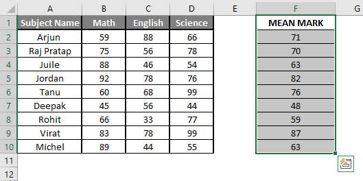
Summary of Example 3: As the user wants to perform the mean calculation for all number in MS Excel. Easley, everything calculated in the above excel example and the Mean is available in the F column.
Things to Remember About How to Find Mean in Excel
- Microsoft Excel’s AVERAGE function used to calculate the Arithmetic Mean of the given input. A user can give 255 input arguments in the function.
- Half the set of a number will be smaller than the mean, and the remaining set will be greater than the mean.
- If a user calculating the normal average, it will exclude the count for a text value, so AVERAGE Mean will bigger than the AVERAGE MEAN.
- Arguments can be number, name, range or cell references that should contain a number.
- If a user wants to calculate the mean with some condition, then use AVERAGEIF or AVERAGEIFS.
Recommended Articles
This is a guide to How to Find Mean in Excel. Here we discuss How to Find Mean along with examples and a downloadable excel template. You may also look at the following articles to learn more –
- FIND Function in Excel
- Excel Find
- Excel Average Formula
- Excel AVERAGE Function
If you have worked with Excel formulas, I am sure you have noticed that sometimes there is a $ symbol as a part of the cell references.
If you’re wondering what does the $ sign means in Excel formulas/functions, this article is the right place.
One of the things that make Excel such a powerful tool is the ability to refer to cells/ranges and use these in formulas.
And when you copy these formulas, these cell references can adjust automatically (or should I say automatically).
Below is an example where I copy the cell C2 (which has a formula) and paste it in C3.
You can see that the formula adjusts the references when I copy and paste it. While in the formula in cell C2 refers to A2 and B2, the one in C3 refers to A3 and B3.
This is called relative reference where the references adjust based on the cell in which it has been applied.
But what if you don’t want some cells to adjust the reference?
What if you want to copy the formula, but don’t want the cell reference to change?
…. introducing the $ sign.
When you use a $ sign before the cell reference (such as $C$2), you’re telling Excel to keep referring to cell C3 even when you copy and paste the formula.
Now you can use the dollar ($) sign in three different ways, which means that there are three types of references on Excel.
Shortcut to add $ Sign to Cell References
There are two ways you can add the $ sign to a cell reference in Excel.
You can either do it manually (i.e., go into the edit mode in a cell by double-clicking on it or using F2, placing the cursor where you want the $ sign and then typing it manually).
Or you can use the keyboard shortcut
F4
To use this shortcut, simply place the cursor on the cell reference where you want to add the dollar sign and press is once. You will notice that it will change the reference by adding/removing the $ sign (based on what’s the original reference).
For example, suppose you have the reference C2 in a cell. Here is how the F4 shortcut would work:
- Press F4 one time – C2 will change to $C$2
- Press F4 two times – C2 will change to C$2
- Press F4 three times – C2 will change to $C2
- Press F4 four times – C2 will change back to C2
Types of References in Excel
There are three types of references in Excel:
- Relative references
- Absolute references
- Mixed references
In relative references, you don’t use a dollar ($) sign in the references at all.
In mixed references, you use the dollar sign ($) only once (such as $C3 or C$3)
In absolute reference, you use the dollar sign in twice in a reference (such as $C$3).
Let me quickly explain each of these with a simple example.
Relative reference
Relative reference is where you don’t use a dollar ($) sign at all.
And when you copy a cell that has a relative reference, it will change and adjust based on the cell where you copy it.
Below is the same example again, where the references adjust as soon as we copy and paste the cell that has the formula.
Absolute reference
In absolute references, you have the $ sign before the row number and the column alphabet (example $C$3)
When you use this in formulas, it will not change the reference
when you copy and paste the cell. This could be useful when you have some value that needs to remain constant (such as time period or interest rates, etc.)
Below is an example where I have a value in cell D2 which needs to remain constant (and not change when we copy-paste the formulas).
By using $D$2, we make sure that it doesn’t change when we copy-paste the cell with the formula.
Note that this example has both, relative cell reference (without the $ sign) and an absolute cell reference (with two $ signs).
Note: If you’re wondering why not simply hard code the value instead of using the absolute cell reference (the one with two dollar signs). While you can use the value itself, in the future, if you have to change the value in formulas, you will have to manually do it. Instead, you can simply change the value in C3, and all the formulas would automatically update.
Mixed reference
These are a little more complicated than the rest two.
In mixed cell references, you will have only one dollar sign (for example – $C3 or C$3)
When you add a dollar sign in front of the column alphabet (C in this example), it locks the column only. This means that if you copy-paste the formula that uses $C3, the column would not change, but the row can change.
And when you add a dollar sign in front of the row number (3 in this example), it locks the column only. This means that if you copy-paste the formula that uses C$3, the row would not change, but the column can change.
Here is a good article that goes in-depth about the mixed cell references in Excel.
Summary
A dollar sign means that the part of the cell reference before which it has been used is anchored or fixed.
Below is a quick summary of what $ means in Excel formulas:
- $A$1 – always refers to column A and row 1
- $A1 – Column A is fixed and will not change, but the row is allowed to change as the formula is copied
- A$1 – Row 1 is fixed and will not change, but the column is allowed to change as the formula is copied.
- $A$1:$A$100 – always refers to the range A1:A100
I hope this article helps you understand what the $ sign means in Excel and how to use it.
Other Excel tutorials you may find useful:
- How to Remove Dollar Sign in Excel
- How to Remove Dashes (-) in Excel?
- How to Lock Cells in Excel [Mac, Windows]
- How to Apply Accounting Number Format in Excel
- What does Pound/Hash Symbol (####) Mean in Excel?
- What Does the Exclamation Point Mean in Excel?
Formulas and functions are the bread and butter of Excel. They drive almost everything interesting and useful you will ever do in a spreadsheet. This article introduces the basic concepts you need to know to be proficient with formulas in Excel. More examples here.
What is a formula?
A formula in Excel is an expression that returns a specific result. For example:
=1+2 // returns 3

=6/3 // returns 2

Note: all formulas in Excel must begin with an equals sign (=).
Cell references
In the examples above, values are «hardcoded». That means results won’t change unless you edit the formula again and change a value manually. Generally, this is considered bad form, because it hides information and makes it harder to maintain a spreadsheet.
Instead, use cell references so values can be changed at any time. In the screen below, C1 contains the following formula:
=A1+A2+A3 // returns 9

Notice because we are using cell references for A1, A2, and A3, these values can be changed at any time and C1 will still show an accurate result.
All formulas return a result
All formulas in Excel return a result, even when the result is an error. Below a formula is used to calculate percent change. The formula returns a correct result in D2 and D3, but returns a #DIV/0! error in D4, because B4 is empty:

There are different ways of handling errors. In this case, you could provide the missing value in B4, or «catch» the error with the IFERROR function and display a more friendly message (or nothing at all).
Copy and paste formulas
The beauty of cell references is that they automatically update when a formula is copied to a new location. This means you don’t need to enter the same basic formula again and again. In the screen below, the formula in E1 has been copied to the clipboard with Control + C:

Below: formula pasted to cell E2 with Control + V. Notice cell references have changed:

Same formula pasted to E3. Cell addresses are updated again:

Relative and absolute references
The cell references above are called relative references. This means the reference is relative to the cell it lives in. The formula in E1 above is:
=B1+C1+D1 // formula in E1
Literally, this means «cell 3 columns left «+ «cell 2 columns left» + «cell 1 column left». That’s why, when the formula is copied down to cell E2, it continues to work in the same way.
Relative references are extremely useful, but there are times when you don’t want a cell reference to change. A cell reference that won’t change when copied is called an absolute reference. To make a reference absolute, use the dollar symbol ($):
=A1 // relative reference
=$A$1 // absolute reference
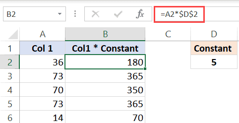
For example, in the screen below, we want to multiply each value in column D by 10, which is entered in A1. By using an absolute reference for A1, we «lock» that reference so it won’t change when the formula is copied to E2 and E3:

Here are the final formulas in E1, E2, and E3:
=D1*$A$1 // formula in E1
=D2*$A$1 // formula in E2
=D3*$A$1 // formula in E3
Notice the reference to D1 updates when the formula is copied, but the reference to A1 never changes. Now we can easily change the value in A1, and all three formulas recalculate. Below the value in A1 has changed from 10 to 12:

This simple example also shows why it doesn’t make sense to hardcode values into a formula. By storing the value in A1 in one place, and referring to A1 with an absolute reference, the value can be changed at any time and all associated formulas will update instantly.
Tip: you can toggle between relative and absolute syntax with the F4 key.
How to enter a formula
To enter a formula:
- Select a cell
- Enter an equals sign (=)
- Type the formula, and press enter.
Instead of typing cell references, you can point and click, as seen below. Note references are color-coded:

All formulas in Excel must begin with an equals sign (=). No equals sign, no formula:

How to change a formula
To edit a formula, you have 3 options:
- Select the cell, edit in the formula bar
- Double-click the cell, edit directly
- Select the cell, press F2, edit directly
No matter which option you use, press Enter to confirm changes when done. If you want to cancel, and leave the formula unchanged, click the Escape key.
Video: 20 tips for entering formulas
What is a function?
Working in Excel, you will hear the words «formula» and «function» used frequently, sometimes interchangeably. They are closely related, but not exactly the same. Technically, a formula is any expression that begins with an equals sign (=).
A function, on the other hand, is a formula with a special name and purpose. In most cases, functions have names that reflect their intended use. For example, you probably know the SUM function already, which returns the sum of given references:
=SUM(1,2,3) // returns 6
=SUM(A1:A3) // returns A1+A2+A3
The AVERAGE function, as you would expect, returns the average of given references:
=AVERAGE(1,2,3) // returns 2
And the MIN and MAX functions return minimum and maximum values, respectively:
=MIN(1,2,3) // returns 1
=MAX(1,2,3) // returns 3
Excel contains hundreds of specific functions. To get started, see 101 Key Excel functions.
Function arguments
Most functions require inputs to return a result. These inputs are called «arguments». A function’s arguments appear after the function name, inside parentheses, separated by commas. All functions require a matching opening and closing parentheses (). The pattern looks like this:
=FUNCTIONNAME(argument1,argument2,argument3)
For example, the COUNTIF function counts cells that meet criteria, and takes two arguments, range and criteria:
=COUNTIF(range,criteria) // two arguments
In the screen below, range is A1:A5 and criteria is «red». The formula in C1 is:
=COUNTIF(A1:A5,"red") // returns 2

Video: How to use the COUNTIF function
Not all arguments are required. Arguments shown in square brackets are optional. For example, the YEARFRAC function returns fractional number of years between a start date and end date and takes 3 arguments:
=YEARFRAC(start_date,end_date,[basis])
Start_date and end_date are required arguments, basis is an optional argument. See below for an example of how to use YEARFRAC to calculate current age based on birthdate.
How to enter a function
If you know the name of the function, just start typing. Here are the steps:
1. Enter equals sign (=) and start typing. Excel will make a list of matching functions based as you type:

When you see the function you want in the list, use the arrow keys to select (or just keep typing).
2. Type the Tab key to accept a function. Excel will complete the function:

3. Fill in required arguments:

4. Press Enter to confirm formula:

Combining functions (nesting)
Many Excel formulas use more than one function, and functions can be «nested» inside each other. For example, below we have a birthdate in B1 and we want to calculate current age in B2:

The YEARFRAC function will calculate years with a start date and end date:

We can use B1 for start date, then use the TODAY function to supply the end date:

When we press Enter to confirm, we get current age based on today’s date:
=YEARFRAC(B1,TODAY())

Notice we are using the TODAY function to feed an end date to the YEARFRAC function. In other words, the TODAY function can be nested inside the YEARFRAC function to provide the end date argument. We can take the formula one step further and use the INT function to chop off the decimal value:
=INT(YEARFRAC(B1,TODAY()))

Here, the original YEARFRAC formula returns 20.4 to the INT function, and the INT function returns a final result of 20.
Notes:
- The current date in images above is February 22, 2019.
- Nested IF functions are a classic example of nesting functions.
- The TODAY function is a rare Excel function with no required arguments.
Key takeaway: The output of any formula or function can be fed directly into another formula or function.
Math Operators
The table below shows the standard math operators available in Excel:
| Symbol | Operation | Example |
|---|---|---|
| + | Addition | =2+3=5 |
| — | Subtraction | =9-2=7 |
| * | Multiplication | =6*7=42 |
| / | Division | =9/3=3 |
| ^ | Exponentiation | =4^2=16 |
| () | Parentheses | =(2+4)/3=2 |
Logical operators
Logical operators provide support for comparisons such as «greater than», «less than», etc. The logical operators available in Excel are shown in the table below:
| Operator | Meaning | Example |
|---|---|---|
| = | Equal to | =A1=10 |
| <> | Not equal to | =A1<>10 |
| > | Greater than | =A1>100 |
| < | Less than | =A1<100 |
| >= | Greater than or equal to | =A1>=75 |
| <= | Less than or equal to | =A1<=0 |
Video: How to build logical formulas
Order of operations
When solving a formula, Excel follows a sequence called «order of operations». First, any expressions in parentheses are evaluated. Next Excel will solve for any exponents. After exponents, Excel will perform multiplication and division, then addition and subtraction. If the formula involves concatenation, this will happen after standard math operations. Finally, Excel will evaluate logical operators, if present.
- Parentheses
- Exponents
- Multiplication and Division
- Addition and Subtraction
- Concatenation
- Logical operators
Tip: you can use the Evaluate feature to watch Excel solve formulas step-by-step.
Convert formulas to values
Sometimes you want to get rid of formulas, and leave only values in their place. The easiest way to do this in Excel is to copy the formula, then paste, using Paste Special > Values. This overwrites the formulas with the values they return. You can use a keyboard shortcut for pasting values, or use the Paste menu on the Home tab on the ribbon.
Video: Paste Special Shortcuts
What’s next?
Below are guides to help you learn more about Excel’s formulas and functions. We also offer online video training.
- 29 tips for working with formulas and functions (video version here)
- 500 formula examples with full explanations
- 101 important Excel functions
- Guide to all Excel functions (work in progress)
- Excel formula errors (examples and fixes)
- Formula criteria — 50 examples
- Formulas for conditional formatting
- How to use F9 to debug a formula (video)
- Excel formula errors and fixes (video)