What is the match function in excel - Word и Excel - помощь в работе с программами

MATCH function

Tip: Try using the new XMATCH function, an improved version of MATCH that works in any direction and returns exact matches by default, making it easier and more convenient to use than its predecessor.

The MATCH function searches for a specified item in a range of cells, and then returns the relative position of that item in the range. For example, if the range A1:A3 contains the values 5, 25, and 38, then the formula =MATCH(25,A1:A3,0) returns the number 2, because 25 is the second item in the range.

Tip: Use MATCH instead of one of the LOOKUP functions when you need the position of an item in a range instead of the item itself. For example, you might use the MATCH function to provide a value for the row_num argument of the INDEX function.

Syntax

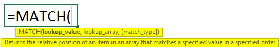
MATCH(lookup_value, lookup_array, [match_type])

The MATCH function syntax has the following arguments:

lookup_value Required. The value that you want to match in lookup_array. For example, when you look up someone’s number in a telephone book, you are using the person’s name as the lookup value, but the telephone number is the value you want.

The lookup_value argument can be a value (number, text, or logical value) or a cell reference to a number, text, or logical value.
lookup_array Required. The range of cells being searched.
match_type Optional. The number -1, 0, or 1. The match_type argument specifies how Excel matches lookup_value with values in lookup_array. The default value for this argument is 1.

The following table describes how the function finds values based on the setting of the match_type argument.

Match_type	Behavior
1 or omitted	MATCH finds the largest value that is less than or equal to *lookup_value. The values in the lookup_array* argument must be placed in ascending order, for example: …-2, -1, 0, 1, 2, …, A-Z, FALSE, TRUE.
0	MATCH finds the first value that is exactly equal to *lookup_value. The values in the lookup_array* argument can be in any order.
-1	MATCH finds the smallest value that is greater than or equal tolookup_value. The values in the *lookup_array* argument must be placed in descending order, for example: TRUE, FALSE, Z-A, …2, 1, 0, -1, -2, …, and so on.

MATCH returns the position of the matched value within lookup_array, not the value itself. For example, MATCH(«b»,{«a»,»b»,»c«},0) returns 2, which is the relative position of «b» within the array {«a»,»b»,»c»}.
MATCH does not distinguish between uppercase and lowercase letters when matching text values.
If MATCH is unsuccessful in finding a match, it returns the #N/A error value.
If match_type is 0 and lookup_value is a text string, you can use the wildcard characters — the question mark (?) and asterisk (*) — in the lookup_value argument. A question mark matches any single character; an asterisk matches any sequence of characters. If you want to find an actual question mark or asterisk, type a tilde (~) before the character.

Example

Copy the example data in the following table, and paste it in cell A1 of a new Excel worksheet. For formulas to show results, select them, press F2, and then press Enter. If you need to, you can adjust the column widths to see all the data.

Product	Count
Bananas	25
Oranges	38
Apples	40
Pears	41
Formula	Description	Result
=MATCH(39,B2:B5,1)	Because there is not an exact match, the position of the next lowest value (38) in the range B2:B5 is returned.	2
=MATCH(41,B2:B5,0)	The position of the value 41 in the range B2:B5.	4
=MATCH(40,B2:B5,-1)	Returns an error because the values in the range B2:B5 are not in descending order.	#N/A

Need more help?

Источник

The MATCH function is used to determine the position of a value in a range or array. For example, in the screenshot above, the formula in cell E6 is configured to get the position of the value in cell D6. The MATCH function returns 5 because the lookup value («peach») is in the 5th position in the range B6:B14:

=MATCH(D6,B6:B14,0) // returns 5

The MATCH function can perform exact and approximate matches and supports wildcards (* ?) for partial matches. There are 3 separate match modes (set by the match_type argument), as described below.

Note: the MATCH function will always return the first match. If you need to return the last match (reverse search) see the XMATCH function. If you want to return all matches, see the FILTER function.

MATCH only supports one-dimensional arrays or ranges, either vertical or horizontal. However, you can use MATCH to locate values in a two-dimensional range or table by giving MATCH the single column (or row) that contains the lookup value. You can even use MATCH twice in a single formula to find a matching row and column at the same time.

Frequently, the MATCH function is combined with the INDEX function to retrieve a value at a certain (matched) position. In other words, MATCH figures out the position, and INDEX returns the value at that position. For a detailed overview with simple examples, see How to use INDEX and MATCH.

Match type information

Match type is optional. If not provided, match_type defaults to 1 (exact or next smallest). When match_type is 1 or -1, it is sometimes referred to as an «approximate match». However, keep in mind that MATCH will always perform an exact match when possible, as noted in the table below:

Match type	Behavior	Details
1	Approximate	MATCH finds the largest value less than or equal to the lookup value. The lookup array must be sorted in ascending order.
0	Exact	MATCH finds the first value equal to the lookup value. The lookup array does not need to be sorted.
-1	Approximate	MATCH finds the smallest value greater than or equal to the lookup value. The lookup array must be sorted in descending order.
(omitted)	Approximate	When match_type is omitted, it defaults to 1 with behavior as explained above.

Caution: Be sure to set match_type to zero (0) if you need an exact match. The default setting of 1 can cause MATCH to return results that look normal but are in fact incorrect. Explicitly providing a value for match_type, is a good reminder of what behavior is expected.

Exact match

When match_type is zero (0), MATCH performs an exact match only. In the example below, the formula in E3 is:

=MATCH(E2,B3:B11,0) // returns 4

In the formula above, the lookup value comes from cell E2. If the lookup value is hardcoded into the formula, it must be enclosed in double quotes («»), since it is a text value:

=MATCH("Mars",B3:B11,0)

Note: MATCH is not case-sensitive, so «Mars» and «mars» will both return 4.

Approximate match

When match_type is set to 1, MATCH will perform an approximate match on values sorted A-Z, finding the largest value less than or equal to the lookup value. In the example shown below, the formula in E3 is:

=MATCH(E2,B3:B11,1) // returns 5

Wildcard match

When match_type is set to zero (0), MATCH can use wildcards. In the example shown below, the formula in E3 is:

=MATCH(E2,B3:B11,0) // returns 6

This is equivalent to:

=MATCH("pq*",B3:B11,0)

INDEX and MATCH

The MATCH function is commonly used together with the INDEX function. The resulting formula is called «INDEX and MATCH». For example, in the screen below, INDEX and MATCH are used to return the cost of a code entered in cell F4. The formula in F5 is:

=INDEX(C5:C12,MATCH(F4,B5:B12,0)) // returns 150

In this example, MATCH is set up to perform an exact match. The MATCH function locates the code ABX-075 and returns its position (7) directly to the INDEX function as the row number. The INDEX function then returns the 7th value from the range C5:C12 as a final result. The formula is solved like this:

=INDEX(C5:C12,MATCH(F4,B5:B12,0))
=INDEX(C5:C12,7)
=150

See below for more examples of the MATCH function. For an overview of how to use INDEX and MATCH with many examples, see: How to use INDEX and MATCH.

Case-sensitive match

The MATCH function is not case-sensitive. However, MATCH can be configured to perform a case-sensitive match when combined with the EXACT function in a generic formula like this:

=MATCH(TRUE,EXACT(lookup_value,array),0))

The EXACT function compares every value in array with the lookup_value in a case-sensitive manner. This formula is explained with an INDEX and MATCH example here.

Notes

MATCH is not case-sensitive.
MATCH returns the #N/A error if no match is found.
MATCH only works with text up to 255 characters in length.
In case of duplicates, MATCH returns the first match.
If match_type is -1 or 1, the lookup_array must be sorted as noted above.
If match_type is 0, the lookup_value can contain the wildcards.
The MATCH function is frequently used together with the INDEX function.

Источник

This Excel tutorial explains how to use the Excel MATCH function with syntax and examples.

Description

The Microsoft Excel MATCH function searches for a value in an array and returns the relative position of that item.

The MATCH function is a built-in function in Excel that is categorized as a Lookup/Reference Function. It can be used as a worksheet function (WS) in Excel. As a worksheet function, the MATCH function can be entered as part of a formula in a cell of a worksheet.

If you want to follow along with this tutorial, download the example spreadsheet.

Download Example

Syntax

The syntax for the MATCH function in Microsoft Excel is:

MATCH( value, array, [match_type] )

Parameters or Arguments

value

The value to search for in the array.

array

A range of cells that contains the value that you are searching for.

match_type

Optional. It the type of match that the function will perform. The possible values are:

match_type	Explanation
1 (default)	The MATCH function will find the largest value that is less than or equal to value. You should be sure to sort your array in ascending order. If the match_type parameter is omitted, it assumes a match_type of 1.
0	The MATCH function will find the first value that is equal to value. The array can be sorted in any order.
-1	The MATCH function will find the smallest value that is greater than or equal to value. You should be sure to sort your array in descending order.

match_type

Explanation

1 (default)

The MATCH function will find the largest value that is less than or equal to value. You should be sure to sort your array in ascending order.

If the match_type parameter is omitted, it assumes a match_type of 1.

The MATCH function will find the first value that is equal to value. The array can be sorted in any order.

-1

The MATCH function will find the smallest value that is greater than or equal to value. You should be sure to sort your array in descending order.

Returns

The MATCH function returns a numeric value.
If the MATCH function does not find a match, it will return a #N/A error.

Note

The MATCH function does not distinguish between upper and lowercase when searching for a match.
If the match_type parameter is 0 and the value is a text value, then you can use wildcards in the value parameter.

Wild card Explanation

* matches any sequence of characters

? matches any single character

Wild card	Explanation
*	matches any sequence of characters
?	matches any single character

Applies To

Excel for Office 365, Excel 2019, Excel 2016, Excel 2013, Excel 2011 for Mac, Excel 2010, Excel 2007, Excel 2003, Excel XP, Excel 2000

Type of Function

Worksheet function (WS)

Example (as Worksheet Function)

Let’s look at some Excel MATCH function examples and explore how to use the MATCH function as a worksheet function in Microsoft Excel:

Based on the Excel spreadsheet above, the following MATCH examples would return:

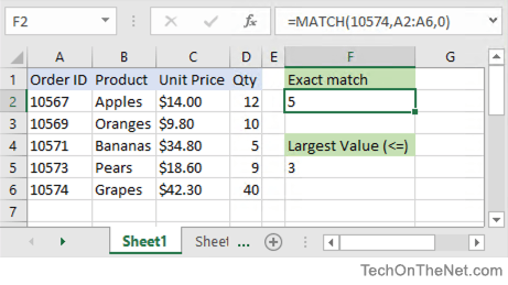
=MATCH(10574,A2:A6,0)
Result: 5     (it matches on 10574)

=MATCH(10572,A2:A6,1)
Result: 3     (it matches on 10571 since the match_type parameter is set to 1)

=MATCH(10572,A2:A6)
Result: 3     (it matches on 10571 since the match_type parameter has been omitted and will default to 1)

=MATCH(10572,A2:A6,0)
Result: #N/A  (it doesn't find a match since the match_type parameter is set to 0)

=MATCH(10573,A2:A6,1)
Result: 4

=MATCH(10573,A2:A6,0)
Result: 4

Let’s look at how we can use wild cards in the MATCH function.

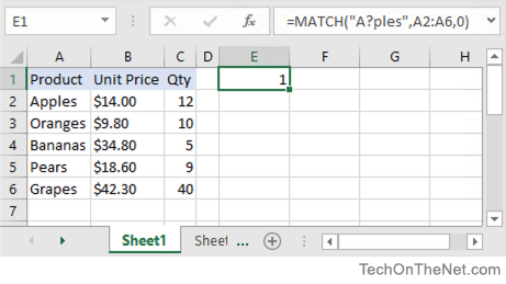
Based on the Excel spreadsheet above, the following MATCH examples would return:

=MATCH("A?ples", A2:A6, 0)
Result: 1

=MATCH("O*s", A2:A6, 0)
Result: 2

=MATCH("O?s", A2:A6, 0)
Result: #N/A

Frequently Asked Questions

Question: In Microsoft Excel, I tried this MATCH formula but it did not work:

=IF(MATCH(B94,Overview!D$54:D$96),"FS","Bulk")

I was hoping for an easier formula than this:

=IF(OR(B94=Overview!D$54,B94=Overview!D55,B94=Overview!D56,  {etc thru D96} ),"FS","Bulk")

Answer: When you are using the MATCH function, you need to be aware of a few things.

First, you need to consider whether your array is sorted in a particular order (ie: ascending order, descending order, or no order). Since we are looking for an exact match and we don’t know if the array is sorted, we want to make sure that the match_type parameter in the MATCH function is set to 0. This will find a match regardless of the sort order.

Second, we know that the MATCH function will return an #N/A error when a match is not found, so we will want to use the ISERROR function to check for the #N/A error.

So based on these 2 additional considerations, we would want to modify your original formula as follows:

=IF(ISERROR(MATCH(B94,Overview!D$54:D$96,0))=FALSE,"FS","Bulk")

This would check for an exact match in the D54:D96 array on the Overview sheet and return «FS» if a match is found. Otherwise, it would return «Bulk» if no match is found.

Question:I have a question about how to nest a MATCH function within the INDEX function. The question is:

I want to create a formula using the MATCH function nested within the INDEX function to retrieve the Class that was selected (by the x) in E4:F10. The MATCH function should find the row where the x is located and should be used within the INDEX function to retrieve the associated Class value from the same row within F4:F10.

Answer:We can use the MATCH function to find the row position in the range E4:E10 to find the row where «x» is located. We then embed this MATCH function within the INDEX function to return the corresponding value in the range F4:$10 as follow:

=INDEX($F$4:$F$10, MATCH("x",$E$4:$E$10))

In this example, we are searching for the value «x» within the range E4:E10. When the value of «x» is found, it will return the corresponding value from F4:F10.

Источник

How to Use the MATCH function in Excel: Step-by-Step

The MATCH function belongs to the list of Excel’s reference/lookup functions. It looks for a value in a lookup array like all the lookup functions do 👀

However, once found, it doesn’t return the corresponding value. But the relative position of the lookup value in the lookup array.

And that’s not it – the MATCH function can do just so much in Excel. So let’s jump into the guide below to learn it all.

Here’s our free sample workbook for this guide for you to download and tag along with the guide ⛵

How to use the MATCH function

The MATCH function of Excel looks for a given value in an array and returns its relative position from that array 🏆

The function is a really simple one, and you’ll enjoy it as we start exploring it. So let’s dive straight into an example.

Here we have a list of students with their scores in English.

It’s hard to find a student from this list readily. And the larger the list grows, the harder it gets 🥴

Do we have a function that can help us find the position of any student from this list readily Let’s try the MATCH function here to find the position of Addams.

Begin writing the MATCH function as follows.

= MATCH (

Write in the lookup_value as the first argument of the MATCH function.

= MATCH (B7

We are looking for the position of Addams – so that makes our lookup value. In this case, our lookup value rests in Cell B7, so we are creating a reference to it.

Refer to the lookup_range as the second argument.

= MATCH (B7, A2:A5

Where should the MATCH function look for the value “Addams”?

This is the table that contains the student names (Cell A2 to Cell A5).

Do not include the headers in this range. If the headers are included in the lookup range, the relative position of the lookup value would be pushed one position down the list.

Kasper Langmann, Microsoft Office Specialist

Define the match_type as 0.

= MATCH (B7, A2:A5, 0)

Pro Tip!

The MATCH function has three different match types 3️⃣

0 – Search for the exact match of the lookup_value.

1 (or omitted) – Search for the largest value less than or equal to the lookup value. The lookup array must be arranged in ascending order for this to work.

-1 – Search for the smallest value greater than or equal to the lookup value. The lookup array must be arranged in descending order for this to work.

The match_type is an optional argument. If omitted, Excel sets it to 1 by default.

For now, we are setting the match_type to 0 as we want Excel to lookup for an exact match. The name Addams is present in the list with the same spelling so the MATCH function can perform an exact match.

Press Enter as we’re done writing the function now 👍

The MATCH function searches and returns the position

And there you go! Excel finds the relative position of Addams from the list of Students.

Addams is in the second position on the list. As the scores next to Addams are arranged in ascending order, this also tells that Addams scored the second least marks among all 🥈

The MATCH function is not a case-sensitive function. It doesn’t differentiate between uppercase and lowercase letters.

Kasper Langmann, Microsoft Office Specialist

Approximate match types

There are three different match types to the MATCH function, and we have only seen one of them yet (the exact match_type).

It’s time that we now look into how the MATCH function works under the other two match types. Let’s take the same example as above – but this time, a little twisted.

For a quick revision, here is the scorecard of the students 📝

Match type (1)

Let’s find which student scored 90 or the next highest mark less than 90.

Must note that for the MATCH function to work with match type 1, the lookup array must be sorted in ascending order.

And take a quick look at our lookup array – it starts from 65 and goes up to 89. Hence, it is already arranged in ascending order.

Kasper Langmann, Microsoft Office Specialist

Write the lookup value of the MATCH function as follows:

= MATCH (B7

We want to find students who scored 90 (or nearest to 90 marks). So that makes up our lookup value.

Write in the lookup array as the next argument.

= MATCH (B7, B2:B5

The score is to be looked up from the column of scores. And so this time our lookup array is B2 to B5 🚀

Set the match type to 1.

= MATCH (B7, B2:B5, 1)

Pro Tip!

Why have we set the match type to 1? That’s because we want to find the student who scored 90 marks. Or if there’s no such student, then we want to find the one who scored the highest marks less than 90.

Under match type 1, the MATCH function search for the largest value less than or equal to the lookup value i.e. 90 🔍

And hit “Enter”.

The MATCH function returns 4. Why is that?

Because we have Cheryl with 89 marks at position 4. None of the students scored 90 marks. And the second highest after 90 is 89 marks 🤩

Match type (-1)

To test match type (-1), let’s find which student scored 80 or the least marks greater than 80.

Must note that for the MATCH function to work with match type -1, the lookup array must be sorted in descending order.

Kasper Langmann, Microsoft Office Specialist

Sort your lookup array in descending order by clicking on the header (Scores here).
Go to Home Tab > Sort and Filter.

Choose Sort Z to A “Highest to Lowest”

Sorting the data from largest to smallest

And you have your list sorted in descending order.

Now, to find the student who scored 80 Marks or the next highest marks:

Write the MATCH function with the following changes from above.

= MATCH (B7, B2:B5, -1)

Our lookup value is now 80. And we have set the match type to -1.

Hit Enter and there comes the results.

The MATCH function returns 2. Why is that?

Because at position 2, we have Ana with 82 marks. After 80, we have 82 on the list (the next highest to our lookup value of 80). That’s match type -1 returns 🎯

Other MATCH formula examples

We yet have more Excel MATCH function examples. Let’s look into them here.

In the image below, we have a list of items with different codes to them 📍

From this list, we want to find the position of the Item “CAR”. But we don’t exactly know the code that suffixes it. How can then we find it?

Under the match type (0), the MATCH function can be used with wildcard characters.

Kasper Langmann, Microsoft Office Specialist

So even if we do not know the exact code after the item name “cars”, we can use a wildcard character. Let’s do it here then:

Write the MATCH function as follows:

= MATCH (

Write the lookup value (Car) as the first argument of the MATCH function.

= MATCH (“Car*”,

As we don’t know the exact code that comes at the end of the item name, we have used an asterisk at the end 😎

An asterisk represents any number of characters at the end of the item name.

Specify the lookup array as the next argument.

= MATCH (“Car*”, A2:A7,

Set the match type to 0.

= MATCH (“Car*”, A2:A7, 0)

And hit “Enter” to get going.

See that? The MATCH function has found the position of Item CAR-34 from the list. Although we never specified the complete name of the item 💪

Pro Tip!

Must note that there were two items by the name CAR in the list. However, the MATCH function returned to position 2 only 🤔

This is because if there are multiple instances of the lookup value in the lookup array, the MATCH function returns the position of the first instance only.

That’s it – Now what

The guide above teaches us the ins and outs of the MATCH function of Excel. We began learning from a simple example of the MATCH function.

And until now we have seen multiple examples of how to use the MATCH function with different match modes.

The MATCH function is a very commonly used function of Excel. It is one of the easier yet very useful functions of Excel.

And that’s not it. There are many more similar useful functions of Excel that you must know about (even if you’re a beginner) 👦

Like the VLOOKUP, SUMIF, and IF functions of Excel. To learn them, enroll in my 30-minute free email course that will teach you these (and many more) functions of Excel.

Other resources

You’d often see the MATCH function is used together with the INDEX function. Both of these functions together to work like an advanced lookup function.

In addition to these, other lookup functions of Excel include the HLOOKUP, VLOOKUP, and XLOOKUP functions of Excel.

Frequently asked question

No. The MATCH function only returns the relative position of a lookup value in a lookup array and not the value itself.

To get the corresponding value for a look-up value, the MATCH function must be used together with the INDEX function.

However, the VLOOKUP function can do all of this alone.

The MATCH function is a lookup/reference function of Excel.

It looks up for a given value in a look-up array. And if found, it returns the relative position of the lookup value in the lookup array.

Kasper Langmann2023-01-11T20:00:46+00:00

Page load link

Источник

What is Match Function in Excel?

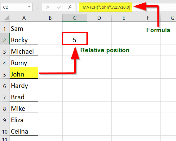
The MATCH function is a powerful tool in Excel that helps users search for a specific value within a range of cells and return its relative position. It’s a useful function for those who work with large datasets or need to locate specific values quickly. For instance, consider a situation where you have a long list of names, and you need to find the position of a particular name (John) within that list. You can use the MATCH function to search for the name and get its position (5).

The utility of the MATCH function extends beyond simple searches within a range. You can use it in conjunction with other functions like INDEX and OFFSET to perform more complex operations.

Key Highlights

The MATCH function in Excel can perform both exact and approximate matches.
It can perform partial matches using wildcard operators such as * and ?.
The MATCH function returns a #N/A error if it doesn’t find a match in the given array.
By using the MATCH and INDEX functions together, we can avoid using the VLOOKUP function to find a value at a matched position.
The Match type is an optional argument in the MATCH function, and if not specified, it defaults to 1.

Syntax of MATCH function in Excel

Lookup_value: It indicates the value whose position we want to find in the selected range. A lookup value can be text, number, logical value, or cell reference.
Lookup_array: It is the cell range that contains the lookup value. Lookup array can be a row or a column.
Match_Type: It is an optional argument with values 1, 0, and -1.

Match_Type “1”: If we set the match type value as 1, Excel provides a value less than or equal to the lookup value.

Match_Type “0”: If we set the match type value as 0, Excel provides the first value that is equal to the lookup value.

Match_Type “-1”: If we set the match type value as 0, Excel provides the smallest value that is greater than or equal to the lookup value.

How to Use Match Function in Excel?

You can download this Match Function in Excel Template here – Match Function in Excel Template

#1 Finding The Exact Match

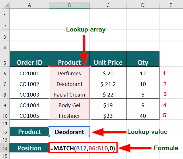
The table below shows a list of ordered products with their order ID, unit price, and sales quantity. We want to find the position of “Deodorant” in the table using the MATCH function in Excel.

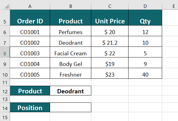
Solution:

Step 1: Select the cell where you want to display the position of the product “Deodorant“. In this case, let’s assume it’s cell B12.

Step 2: Type the MATCH function in the formula bar: =MATCH(B12,B6:B10,0)

The first argument in the formula is the lookup value, which is “Deodorant“, i.e., cell B12.
The second argument of the MATCH function is the lookup array, which is the range B6:B10. This range contains the products listed in the table.

Note: The lookup_array can be a row or a column.

The third argument of the MATCH function is the match type, which is 0. This means we want to find an exact match of the lookup value in the array.

Step 3: Press Enter to get the result, as shown below.

result

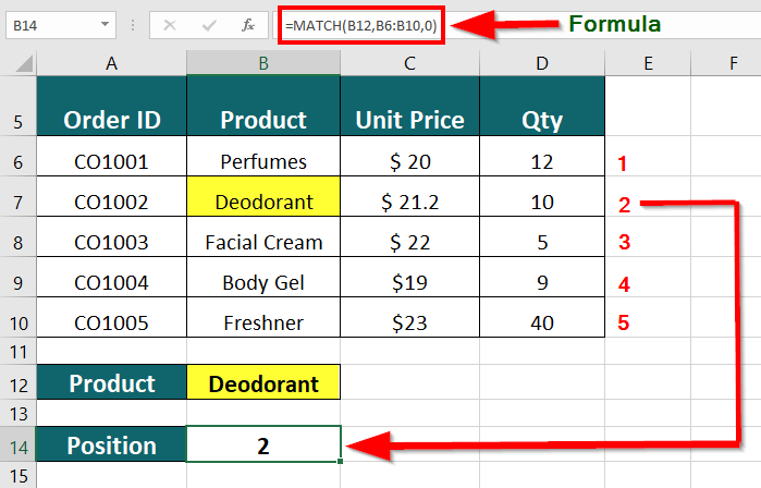
The formula returns the position of “Deodorant” in the table, which is 2. This means that “Deodorant” is the second product listed in the table.

Explanation of the formula:

When you press the Enter key, Excel searches through the cells in the lookup array “B6:B10” to find an exact match for the lookup value “Deodorant”. After finding the match, it returns the position of the first cell containing the lookup value. In this scenario, the formula returns the value “2“, indicating that the first cell containing “Deodorant” is the second cell in the range B6:B10.

#2 Finding Partial Match using Wildcard Character

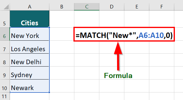
Let’s say we have a list of cities in Column A, and we want to find the position of the city that starts with “New” in the list.

Here’s how we can do it:

Step 1: Open a new Excel spreadsheet and enter the list of cities in Column A.

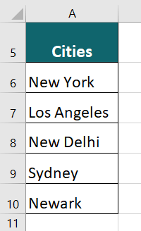
Step 2: In an empty cell, enter the formula =MATCH(“New*”,A6:A10,0).

Explanation of the formula:

“New*”: This is the search criteria. The asterisk () is a wildcard character representing any number of characters. So, “New” will match any city name that starts with “New”.
A6:A10: This is the range of cells we want to search for our city name in.
0: This is the match_type argument. Here, we’re using an exact match, so we specify 0.

step 2

Step 3: Press the “Enter” key to display the result in the cell where you entered the formula.

step 3

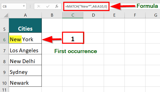
The result is “1,” which is the position of the first city that starts with “New”. In this case, “New York” is the first city that starts with “New” in the list.

Note: If multiple cities match the search criteria, the MATCH function will only return the position of the first occurrence.

#3 Using INDEX and MATCH Function Together

The table below shows a list of students with their marks in the subjects – Language, Maths, History, and Physics. Using the INDEX and MATCH functions together, we want to find Alex’s marks in History

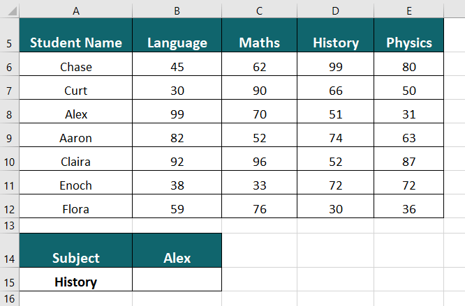
Solution:

Step 1: Select the cell where you want to display the result. In this case, it is cell B15.

Step 2: Enter the formula in the cell:

=INDEX(A5:E12,MATCH(B14,A5:A12,0),MATCH(A15,A5:E5,0))

A5:E12: This is the range of cells containing the table of student data.
B14: This is the value we want to find in the first column of the table, which is the name of the student whose marks we want to find (in this case, “Alex”).
A5:A12: This is the range of cells containing the students’ names in the table’s first column.
0: This argument specifies that we want an exact match.
A15: This is the value we’re looking for in row 5, which is the subject “History”.
A5:E5: This is the cell range containing the subject names.

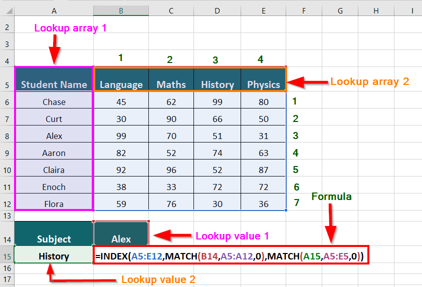
Step 3: Press Enter key to get the below result.

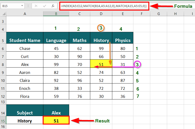
The INDEX and MATCH functions of Excel work together to provide the result of 51, which denote History marks of Alex.

Explanation of how the formula works:

The first MATCH function in the formula =INDEX(A5:E12,MATCH(B14,A5:A12,0),MATCH(A15,A5:E5,0)) searches for the student name “Alex” in the range A5:A12 and returns the relative position of that name within the range. The third argument of the MATCH function is 0, which specifies that we want an exact match. In this case, “Alex” is in the third row of the range, so the first MATCH function returns the value 3.
The second MATCH function in the formula searches for the subject “History” in the range A5:E5 and returns the relative position of that subject within the range. Again, the third argument of the MATCH function is 0, which specifies that we want an exact match. In this case, “History” is in the third column of the range, so the second MATCH function returns the value 3.
The INDEX function then uses these two values (3 and 3) to return the corresponding value in the table, which is the marks that Alex scored in History (51).

Things to Remember
- Match types: You can use three match types with the MATCH function: 0, 1, and -1. The default match type is 0, which finds an exact match. Match type 1 finds the largest value that is less than or equal to the lookup_value, while match type -1 finds the smallest value that’s greater than/ equal to the lookup_value.
- Array size: The lookup_array argument must be a one-dimensional array or a reference to a one-dimensional range of cells. If the lookup_array is not one-dimensional, the MATCH function will return a #N/A error.
- Sorted order: If the values in the lookup_array are not sorted in ascending order, the MATCH function in Excel may return an incorrect result. In such cases, use the match_type argument to specify the appropriate match type.
- Exact match: If the MATCH function does not find the lookup_value in the lookup_array, it will return a #N/A error. You can use the IFERROR function to handle this error and return a more meaningful result.
- Relative or absolute cell reference: The MATCH function is compatible with both relative and absolute cell references. When copying the formula to other cells, the function will adjust the cell references accordingly.

Frequently Asked Questions (FAQs)

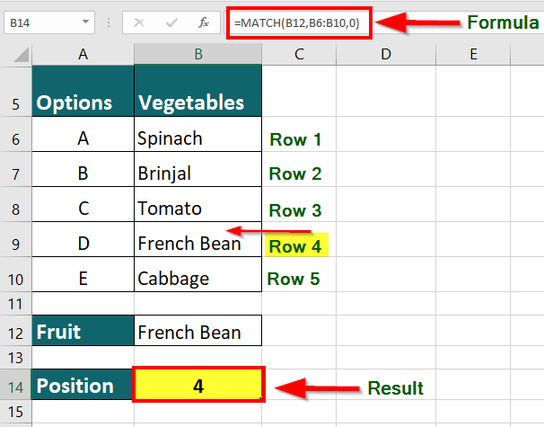
Q1. What is example of a MATCH function in Excel?
Answer: The MATCH function searches for a given value in a data set and provides the position of that value in the range. For instance, suppose you have a data set that includes items like Spinach, Brinjal, Tomato, French Bean, and Cabbage in the range B6:B10. If you want to find the position of the value “French Bean” in the range, you can use the MATCH function.

The formula =MATCH(B12,B6:B10,0) returns the “French Bean” position in the range B6:B10 as the number 4.

Q2. What is the benefit of including the MATCH function within an INDEX function?
Answer: Including the MATCH function within an INDEX function allows you to retrieve data dynamically based on specific search criteria.

Suppose you have a list of fruits and their prices in a table. You want to retrieve the price of a specific fruit, say “Apple”, from the table. One way to do this is to manually search the table for the row containing “Apple”, and then look for the price in the corresponding column. However, if you have a large dataset with many rows and columns, this can be a time-consuming and error-prone process. Instead, you can use the MATCH function to find the row number of “Apple” in the table and then use the INDEX function to retrieve the price from the corresponding column. The formula would look like this:

=INDEX(B2:E6,MATCH(“Apple”,A2:A6,0),3)

The MATCH function searches for “Apple” in the first column (A2:A6) of the table and returns the row number where it is found. The INDEX function then retrieves the value from the table’s third column (price column) at the intersection of the row number and column number that the MATCH function returns.

Q3. Can the MATCH function have multiple criteria?
Answer: It is possible to use the MATCH function with multiple criteria by combining it with other functions such as INDEX, SUMPRODUCT, and COUNTIFS. For instance, consider this formula:

= MATCH(1, (B2:B10=”Sales”) * (C2:C10>20000), 0) + COUNTIFS(B2:B10, “Sales”, C2:C10, “>20000”)

This formula uses MATCH with multiple criteria to find the position of the first employee in the “Sales” department who earns more than $20,000 per year. Then, it adds the count of cells that satisfy only the second condition using the COUNTIFS function.

Q4. What is the difference between MATCH and VLOOKUP in Excel?
Answer: The MATCH function helps us find the location of a particular value in a column or row, while the VLOOKUP function helps us retrieve information associated with that value.

For instance, if we want to find the price of oranges in the following table, we will have to use the MATCH function in conjunction with the INDEX function to find the price. Alternatively, the VLOOKUP function can directly provide the price of oranges at $0.75.

Product Price

Apples $1.00

Oranges $0.75

Bananas $0.50
- The formula for using MATCH and INDEX functions together is =INDEX(B:B, MATCH(“Oranges”, A:A, 0)). Using MATCH, this formula finds the position of “Oranges” in column A, which returns the value 2. Then, INDEX retrieves the value in column B’s corresponding row, which is $0.75.
- The VLOOKUP function formula is =VLOOKUP(“Oranges”, A:B, 2, 0). This formula looks for “Oranges” in the first column of the range A:B, and returns the corresponding value from the second column (which is the price column), resulting in $0.75.

The Syntax of the MATCH Excel Function

The syntax of the function is shown in the following image:

The function accepts the following arguments:

Lookup_value: This is the value to be searched in the “lookup_array.”
Lookup_array: This is the array or range of cells where the “lookup_value” is to be searched.
Match_type: This takes the values 1, 0, or -1 depending on the type of match.

For instance, you may want to search a specific word (lookup_value) in the dictionary (lookup_array).

The arguments “lookup_value” and “lookup_array” are mandatory, while “match_type” is optional.

The Values of “Match_Type”

The “match_type” can take any of the following values:

Positive one (1): The function looks for the largest value in the “lookup_array,” which is less than or equal to the “lookup_value.” The data is arranged in alphabetical (A to Z) or ascending order and an approximate match is returned.

Zero (0): The function looks for an exact match of the “lookup_value” in the “lookup_array.” The data is not required to be arranged.

Negative one (-1): The function looks for the smallest value in the “lookup_array,” which is greater than or equal to the “lookup_value.” The data is arranged in reverse order of alphabets (Z to A) or descending order and an approximate match is returned.

Note: The default value of “match_type” is 1.

How to use the MATCH Function in Excel? (With Examples)

Let us understand the working of the MATCH formula with the help of examples.

You can download this MATCH Function Excel Template here – MATCH Function Excel Template

Example #1–Exact Match

The succeeding table shows the serial number (S.N.), name, and department of ten employees in an organization. We want to find the position of the employee “Tanuj.”

We apply the following formula.

“=MATCH(F4,$B$4:$B$13,0)”

The “match_type” is set at 0 to return the exact position of “Tanuj” (lookup_value) from the range $B$4:$B$13 (lookup_array). The output is 1.

Example #2–Approximate Match

The succeeding list shows the values from 100 to 1000. We want to find the approximate position of the value 525.

We apply the following formula.

“=MATCH(E19,B19:B28,1)”

The “match_type” is set at 1 to return the approximate match of 525 (lookup_value) from the range B19:B28 (lookup_array).

The MATCH function looks for the largest value (500), which is less than 525 in the given array. Hence, the output is 5.

Example #3–Wildcard Character (Partial Match)

The MATCH function supports the usage of wildcard charactersIn Excel, wildcards are the three special characters asterisk, question mark, and tilde. Asterisk denotes multiple characters, a question mark denotes a single character, and a tilde denotes the identification of a wild card character.read more (? and *) in the “lookup_value” argument. Let us consider an example of the same.

The succeeding list shows ten IDs of the various employees of an organization. We want to find the position of the ID ending with 105.

We apply the following formula.

“=MATCH(“*”&E33,$B$33:$B$42,0)”

The wildcard characters are used for partial matches and the “match_type” is set at zero. The output is 5. This implies that the ID at the fifth position is ending with 105.

Example 4–INDEX MATCH

The MATCH and INDEX functionThe INDEX function can return the result from the row number, and the MATCH function can give us the position of the lookup value in the array. This combination of the INDEX MATCH is beneficial in addressing a fundamental limitation of VLOOKUP.read more are used together to look up a value in the table from right to left.

The succeeding table shows the serial number (S.N.), name, and department of ten employees in an organization. We want to find the serial number of the employee “Tanuj.”

We apply the following formula.

“=INDEX(B46:D56,MATCH(G48,C46:C56,0),1)”

The MATCH function searches for the exact word “Tanuj” in the range C46:C56 and returns 2. The output 2 is supplied as the row number to the INDEX functionThe INDEX function in Excel helps extract the value of a cell, which is within a specified array (range) and, at the intersection of the stated row and column numbers.read more. The INDEX function returns the value from the second row and first column of the range B46:D56.

The output of the formula is 1. This implies that the serial number of “Tanuj” is 1.

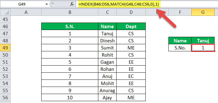
The following image shows the output when the “lookup_value” is “Tanujh.” Since “Tanujh” could not be found in column B, the outcome is “#N/A” error.

The Properties of the MATCH Excel Function

It is not case-sensitive which implies that it does not distinguish between the uppercase and lowercase letters.
It returns the relative position of the “lookup_value” in the “lookup_array.”
It works with one-dimensional ranges or arrays which can be either vertical or horizontal.
If there are multiple occurrences of the “lookup_value” in the “lookup_array,” it returns the position of the first exact match.
If the “lookup_value” is in text form, the wildcard characters like a question mark (?) and asterisk (*) can be used for partial matches.
It returns the “#N/A” error if it is unable to find the “lookup_value” in the “lookup_array.”

Frequently Asked Questions

1. Define the MATCH function of Excel.

The MATCH function returns the position of a given value from a vertical or horizontal array or range of cells. It returns both approximate and exact matches from unsorted and sorted data lists respectively.

The MATCH function can be used in combination with the INDEX function to extract a value from the position supplied by the former. The MATCH function accepts the arguments “lookup_value,” “lookup_array,” and “match_type.”

The first two arguments are mandatory, while the last is optional. The “match_type” can take the values 1, 0 or -1 depending on the type of match. The value 0 refers to an exact match, while 1 and -1 refer to an approximate match.

2. How is the MATCH function used to compare two columns in Excel?

The MATCH function is used in combination with the IF and ISNA functions to compare two columns. The formula is stated as follows:

“IF(ISNA(MATCH(first value in list1,list2,0)),“not in list 1”,“”)”

The formula looks for a value of “list 1” in “list 2.” If it is able to find a value, its relative position is returned. However, if a value of “list 2” is not present in “list 1,” the formula returns the text “not in list 1.”

3. What is the INDEX MATCH formula of Excel?

The INDEX MATCH formula uses a combination of the INDEX and MATCH functions. The INDEX function looks for a value in an array based on the specified row and column numbers. These row and column numbers are supplied by the MATCH function.

The INDEX MATCH formula for a vertical lookup is stated as follows:

“INDEX(column to return a value from,MATCH(lookup_value,column to look up against,0)”

The “column to return a value from” is the “array” argument of the INDEX function. The “column to look up against” is the “lookup_array” argument of the MATCH function.

Note: The “array” argument of the INDEX function must contain the same number of rows as the “lookup_array” argument of the MATCH function.

Excel Match Function Definition:

Excel defines match function as: “Returns the relative position of an item in an array that matches a specified value in a specified order”. In simple plain language Match function searches for a value in a defined range and then returns its position.

Syntax of Match Formula:

Match formula can be written as: MATCH(lookup_value, range, match_type)

Here: ‘lookup_value’ signifies the value to be searched in the array.

‘range’ is the array of values on which you want to perform a match.

‘match_type’ Match type is an important thing. It can have three values 1, 0 or -1.

If ‘match_type’ has a value 1, it means that match function will find a value that is less than or equal to ‘lookup_value’. It can only be applied if the array (‘range’) is sorted in an ascending order.
If ‘match_type’ has a value 0, it means that match function will find the first value that is equal to the ‘lookup_value’. In this case sorting of array (‘range’) is not important.
If ‘match_type’ has a value -1, it means that match function will find the smallest value that is greater than or equal to ‘lookup_value’. It can only be applied if the array (‘range’) is sorted in a descending order.

Few Important things about Match Formula:

Match is case-insensitive. It does not know the difference between upper and lower case.
If ‘match_type’ i.e. the third parameter of match function is omitted, then the function treats its value to be 1 as default.
If the Match formula cannot find any matches, it results into #N/A error.
Match function also supports the use of wildcard operators, but they can only be used in case of text comparisons where the ‘match_type’ is 0. We will cover this with an example later.
Match function does not return the matching string, it only returns the relative position of that string.
If the array is not sorted in the ascending order for ‘match_type’ 1 then it results into a #N/A error. Similarly #N/A error also occurs if the defined cell range is not sorted in descending order for ‘match_type’ equal to -1.

Example of Match Formula in Excel:

In the first example we have applied a Match function as shown in the above image.

The Match Function is applied as: =MATCH(104,B2:B8,1)

The Result is 3.

This means that Match searches the whole range for the value 104 but as 104 was not present in the list so it pointed to the relative position of a value slightly less than 104 i.e. 103. If in the same example the array would have the value 104 with array being sorted in ascending order then the same formula would have resulted into pointing the relative reference of 104.

If we apply another Match function: =MATCH(104,B2:B8,0) on the same data set.

Then it will result into an error as ‘0’ signifies exact match and in absence of the value 104 the function will give an error #N/A

If we apply another Match function: =MATCH(104,B2:B8,-1) on the same data set.

Then it will result into an error as the array is not sorted in descending order.

In the second example a Match formula with match type as -1 is used.

The Result is: 4

This is because as the value 104 is not present in the array so the Match function points to the relative reference of a value slightly greater than 104 i.e. 105.

WildCard Operators in Match Function:

Using wildcards can only prove useful in the case of exact string matches i.e. ‘match_type’ 0. Generally two types of wildcard operators can be used within the Match Function.

“?” Wildcard: This signifies any single character.
“*” Wildcard: This signifies any number of characters.

In the above example we have applied a Match Formula as: =MATCH("T?a",A2:A8,0)

The ‘lookup_value’ contains the “?” wildcard operator which matches the array element “Tea” and hence the result of match function is the relative position of “Tea” i.e. 3

If another Match function: =MATCH("C*e",A2:A8,0) is applied on the same dataset. Then it will result into a value 7. As “C*e” matches “coffee” and hence the Match function gives the relative position of “Coffee” element in the array.

So, this was all about Match function in Excel. Do let me know if you have any queries about this wonderful function.

Источник

Date yes Add (Subtract) Days to a Date Concatenate Dates Convert Date to Number Convert Date to Text Month Name to Number Create Date Range from Dates Day Number of Year Month Name from Date First Day of Month Add (Subtract) Weeks to a Date If Functions with Dates Max Date Number of Days Between Dates Number of Days in a Month Number of Weeks Between Dates Number of Years Between Dates Split Date & Time into Separate Cells Countdown Remaining Days Insert Dates Random Date Generator Using Dynamic Ranges — Year to Date Values Add (Subtract) Years to a Date Date Formula Examples Extract Day from Date Get Day Name from Date Count Days Left in Month / Year Count Workdays Left in Month / Year Get Last Day of Month Last Business Day of Month / Year Number of Work / Business Days in Month Weekday Abbreviations Auto Populate Dates Number of Months Between Dates Quarter from a Date Years of Service Change Date Format Compare Dates Time yes Add (Subtract) Hours to Time Add (Subtract) Minutes to Time Add (Subtract) Seconds to Time Add Up time (Total Time) Time Differences Change Time Format Convert Minutes to Hours Convert Time to Decimal Convert Time to Hours Convert Time to Minutes Convert Time to Seconds Military Time Round Time to Nearest 15 Minutes Overtime Calculator Number of Hours Between Times Convert Seconds to Minutes, Hours, or Time Count Hours Worked Time Differences Time Format — Show Minutes Seconds Text yes Add Commas to Cells Get First Word from Text Capitalize First Letter Clean & Format Phone #s Remove Extra Trailing / Leading Spaces Add Spaces to Cell Assign Number Value to Text Combine Cells with Comma Combine First and Last Names Convert Text String to Date Convert Text to Number Extract Text From Cell Get Last Word Remove Unwated Characters Extract Text Before or After Character How to Split Text String by Space, Comma, & More Remove Special Characters Remove First Characters from Left Substitute Multiple Values Switch First & Last Names w/ Commas Remove Specific Text from a Cell Extract Text Between Characters (Ex. Parenthesis) Add Leading Zeros to a Number Remove Line Breaks from Text Remove all Numbers from Text Reverse Text Remove Non-Numeric Characters Remove Last Character(s) From Right Separate First and Last Names Separate Text & Numbers Round yes Round Formulas Round Price to Nearest Dollar or Cent Round to Nearest 10, 100, or 1000 Round to Nearest 5 or .5 Round Percentages Round to Significant Figures Count yes Count Blank and Non-blank Cells Count Cells Between Two Numbers Count Cells not Equal to Count if Cells are in Range Count Times Word Appears in Cell Count Words in Cell Count Specific Characters in Column Count Total Number of Characters in Column Count Cells that Equal one of two Results Count Cells that do not Contain Count Cells that Contain Specific Text Count Unique Values in Range Countif — Multiple Criteria Count Total Number of Cells in Range Count Cells with Any Text Count Total Cells in a Table Lookup yes Two Dimensional VLOOKUP VLOOKUP Simple Example Vlookup — Multiple Matches Case Sensitive Lookup Case Sensitive VLOOKUP Sum if — VLOOKUP Case Sensitive Lookup Case Sensitive VLOOKUP Find Duplicates w/ VLOOKUP or MATCH INDEX MATCH MATCH Lookup — Return Cell Address (Not Value) Lookup Last Value in Column or Row Reverse VLOOKUP (Right to Left) Risk Score Bucket with VLOOKUP Sum with a VLOOKUP Function VLOOKUP & INDIRECT VLOOKUP Concatenate VLOOKUP Contains (Partial Match) 17 Reasons Why Your XLOOKUP is Not Working Double (Nested) XLOOKUP — Dynamic Columns IFERROR (& IFNA) XLOOKUP Lookup Min / Max Value Nested VLOOKUP Top 11 Alternatives to VLOOKUP (Updated 2022!) VLOOKUP – Dynamic Column Reference VLOOKUP – Fix #N/A Error VLOOKUP – Multiple Sheets at Once VLOOKUP & HLOOKUP Combined VLOOKUP & MATCH Combined VLOOKUP Between Worksheets or Spreadsheets VLOOKUP Duplicate Values VLOOKUP Letter Grades VLOOKUP Return Multiple Columns VLOOKUP Returns 0? Return Blank Instead VLOOKUP w/o #N/A Error XLOOKUP Multiple Sheets at Once XLOOKUP Between Worksheets or Spreadsheets XLOOKUP by Date XLOOKUP Duplicate Values XLOOKUP Multiple Criteria XLOOKUP Return Multiple Columns XLOOKUP Returns 0? Return Blank Instead XLOOKUP Text XLOOKUP with IF XLOOKUP With If Statement Misc. yes Sort Multiple Columns Use Cell Value in Formula Percentage Change Between Numbers Percentage Breakdown Rank Values Add Spaces to Cell CAGR Formula Average Time Decimal Part of Number Integer Part of a Number Compare Items in a List Dealing with NA() Errors Get Worksheet Name Wildcard Characters Hyperlink to Current Folder Compound Interest Formula Percentage Increase Create Random Groups Sort with the Small and Large Functions Non-volatile Function Alternatives Decrease a Number by a Percentage Calculate Percent Variance Profit Margin Calculator Convert Column Number to Letter Get Full Address of Named Range Insert File Name Insert Path Latitute / Longitude Functions Replace Negative Values Reverse List Range Convert State Name to Abbreviation Create Dynamic Hyperlinks Custom Sort List with Formula Data Validation — Custom Formulas Dynamic Sheet Reference (INDIRECT) Reference Cell in Another Sheet or Workbook Get Cell Value by Address Get Worksheet Name Increment Cell Reference List Sheet Names List Skipped Numbers in Sequence Return Address of Max Value in Range Search by Keywords Select Every Other (or Every nth) Row Basics yes Cell Reference Basics — A1, R1C1, 3d, etc. Add Up (Sum) Entire Column or Row Into to Dynamic Array Formulas Conversions yes Convert Time Zones Convert Celsius to Fahrenheit Convert Pounds to Kilograms Convert Time to Unix Time Convert Feet to Meters Convert Centimeters to Inches Convert Kilometers to Miles Convert Inches to Feet Convert Date to Julian Format Convert Column Letter to Number Tests yes Test if a Range Contains any Text Test if any Cell in Range is Number Test if a Cell Contains a Specific Value Test if Cell Contains Any Number Test if Cell Contains Specific Number Test if Cell is Number or Text If yes Percentile If Subtotal If Sumproduct If Large If and Small If Median If Concatentate If Max If Rank If TEXTJOIN If Sum yes Sum if — Begins With / Ends With Sum if — Month or Year to Date Sum if — By Year Sum if — Blank / Non-Blank Sum if — Horizontal Sum Count / Sum If — Cell Color INDIRECT Sum Sum If — Across Multiple Sheets Sum If — By Month Sum If — Cells Not Equal To Sum If — Not Blank Sum if — Between Values Sum If — Week Number Sum Text Sum if — By Category or Group Sum if — Cell Contains Specific Text (Wildcards) Sum if — Date Rnage Sum if — Dates Equal Sum if — Day of Week Sum if — Greater Than Sum if — Less Than Average yes Average Non-Zero Values Average If — Not Blank Average — Ignore 0 Average — Ignore Errors Math yes Multiplication Table Cube Roots nth Roots Square Numbers Square Roots Calculations yes Calculate a Ratio Calculate Age KILLLLLLL Calculate Loan Payments GPA Formula Calculate VAT Tax How to Grade Formulas Find yes Find a Number in a Column / Workbook Find Most Frequent Numbers Find Smallest n Values Find nth Occurance of Character in Text Find and Extract Number from String Find Earliest or Latest Date Based on Criteria Find First Cell with Any Value Find Last Row Find Last Row with Data Find Missing Values Find Largest n Values Most Frequent Number Conditional Formatting yes Conditional Format — Dates & Times Conditional Format — Highlight Blank Cells New Functions XLOOKUP Replaces VLOOKUP, HLOOKUP, and INDEX / MATCH Logical yes AND Checks whether all conditions are met. TRUE/FALSE IF If condition is met, do something, if not, do something else. IFERROR If result is an error then do something else. NOT Changes TRUE to FALSE and FALSE to TRUE. OR Checks whether any conditions are met. TRUE/FALSE XOR Checks whether one and only one condition is met. TRUE/FALSE Lookup & Reference yes FALSE The logical value: FALSE. TRUE The logical value: TRUE. ADDRESS Returns a cell address as text. AREAS Returns the number of areas in a reference. CHOOSE Chooses a value from a list based on it’s position number. COLUMN Returns the column number of a cell reference. COLUMNS Returns the number of columns in an array. HLOOKUP Lookup a value in the first row and return a value. HYPERLINK Creates a clickable link. INDEX Returns a value based on it’s column and row numbers. INDIRECT Creates a cell reference from text. LOOKUP Looks up values either horizontally or vertically. MATCH Searches for a value in a list and returns its position. OFFSET Creates a reference offset from a starting point. ROW Returns the row number of a cell reference. ROWS Returns the number of rows in an array. TRANSPOSE Flips the oriention of a range of cells. VLOOKUP Lookup a value in the first column and return a value. Date & Time yes DATE Returns a date from year, month, and day. DATEDIF Number of days, months or years between two dates. DATEVALUE Converts a date stored as text into a valid date DAY Returns the day as a number (1-31). DAYS Returns the number of days between two dates. DAYS360 Returns days between 2 dates in a 360 day year. EDATE Returns a date, n months away from a start date. EOMONTH Returns the last day of the month, n months away date. HOUR Returns the hour as a number (0-23). MINUTE Returns the minute as a number (0-59). MONTH Returns the month as a number (1-12). NETWORKDAYS Number of working days between 2 dates. NETWORKDAYS.INTL Working days between 2 dates, custom weekends. NOW Returns the current date and time. SECOND Returns the second as a number (0-59) TIME Returns the time from a hour, minute, and second. TIMEVALUE Converts a time stored as text into a valid time. TODAY Returns the current date. WEEKDAY Returns the day of the week as a number (1-7). WEEKNUM Returns the week number in a year (1-52). WORKDAY The date n working days from a date. WORKDAY.INTL The date n working days from a date, custom weekends. YEAR Returns the year. YEARFRAC Returns the fraction of a year between 2 dates. Engineering yes CONVERT Convert number from one unit to another. Financial yes FV Calculates the future value. PV Calculates the present value. NPER Calculates the total number of payment periods. PMT Calculates the payment amount. RATE Calculates the interest Rate. NPV Calculates the net present value. IRR The internal rate of return for a set of periodic CFs. XIRR The internal rate of return for a set of non-periodic CFs. PRICE Calculates the price of a bond. YIELD Calculates the bond yield. INTRATE The interest rate of a fully invested security. Information yes CELL Returns information about a cell. ERROR.TYPE Returns a value representing the cell error. ISBLANK Test if cell is blank. TRUE/FALSE ISERR Test if cell value is an error, ignores #N/A. TRUE/FALSE ISERROR Test if cell value is an error. TRUE/FALSE ISEVEN Test if cell value is even. TRUE/FALSE ISFORMULA Test if cell is a formula. TRUE/FALSE ISLOGICAL Test if cell is logical (TRUE or FALSE). TRUE/FALSE ISNA Test if cell value is #N/A. TRUE/FALSE ISNONTEXT Test if cell is not text (blank cells are not text). TRUE/FALSE ISNUMBER Test if cell is a number. TRUE/FALSE ISODD Test if cell value is odd. TRUE/FALSE ISREF Test if cell value is a reference. TRUE/FALSE ISTEXT Test if cell is text. TRUE/FALSE N Converts a value to a number. NA Returns the error: #N/A. TYPE Returns the type of value in a cell. Math yes ABS Calculates the absolute value of a number. AGGREGATE Define and perform calculations for a database or a list. CEILING Rounds a number up, to the nearest specified multiple. COS Returns the cosine of an angle. DEGREES Converts radians to degrees. DSUM Sums database records that meet certain criteria. EVEN Rounds to the nearest even integer. EXP Calculates the exponential value for a given number. FACT Returns the factorial. FLOOR Rounds a number down, to the nearest specified multiple. GCD Returns the greatest common divisor. INT Rounds a number down to the nearest integer. LCM Returns the least common multiple. LN Returns the natural logarithm of a number. LOG Returns the logarithm of a number to a specified base. LOG10 Returns the base-10 logarithm of a number. MOD Returns the remainder after dividing. MROUND Rounds a number to a specified multiple. ODD Rounds to the nearest odd integer. PI The value of PI. POWER Calculates a number raised to a power. PRODUCT Multiplies an array of numbers. QUOTIENT Returns the integer result of division. RADIANS Converts an angle into radians. RAND Calculates a random number between 0 and 1. RANDBETWEEN Calculates a random number between two numbers. ROUND Rounds a number to a specified number of digits. ROUNDDOWN Rounds a number down (towards zero). ROUNDUP Rounds a number up (away from zero). SIGN Returns the sign of a number. SIN Returns the sine of an angle. SQRT Calculates the square root of a number. SUBTOTAL Returns a summary statistic for a series of data. SUM Adds numbers together. SUMIF Sums numbers that meet a criteria. SUMIFS Sums numbers that meet multiple criteria. SUMPRODUCT Multiplies arrays of numbers and sums the resultant array. TAN Returns the tangent of an angle. TRUNC Truncates a number to a specific number of digits. Stats yes AVERAGE Averages numbers. AVERAGEA Averages numbers. Includes text & FALSE =0, TRUE =1. AVERAGEIF Averages numbers that meet a criteria. AVERAGEIFS Averages numbers that meet multiple criteria. CORREL Calculates the correlation of two series. COUNT Counts cells that contain a number. COUNTA Count cells that are non-blank. COUNTBLANK Counts cells that are blank. COUNTIF Counts cells that meet a criteria. COUNTIFS Counts cells that meet multiple criteria. FORECAST Predict future y-values from linear trend line. FREQUENCY Counts values that fall within specified ranges. GROWTH Calculates Y values based on exponential growth. INTERCEPT Calculates the Y intercept for a best-fit line. LARGE Returns the kth largest value. LINEST Returns statistics about a trendline. MAX Returns the largest number. MEDIAN Returns the median number. MIN Returns the smallest number. MODE Returns the most common number. PERCENTILE Returns the kth percentile. PERCENTILE.INC Returns the kth percentile. Where k is inclusive. PERCENTILE.EXC Returns the kth percentile. Where k is exclusive. QUARTILE Returns the specified quartile value. QUARTILE.INC Returns the specified quartile value. Inclusive. QUARTILE.EXC Returns the specified quartile value. Exclusive. RANK Rank of a number within a series. RANK.AVG Rank of a number within a series. Averages. RANK.EQ Rank of a number within a series. Top Rank. SLOPE Calculates the slope from linear regression. SMALL Returns the kth smallest value. STDEV Calculates the standard deviation. STDEV.P Calculates the SD of an entire population. STDEV.S Calculates the SD of a sample. STDEVP Calculates the SD of an entire population TREND Calculates Y values based on a trendline. Text yes CHAR Returns a character specified by a code. CLEAN Removes all non-printable characters. CODE Returns the numeric code for a character. CONCATENATE Combines text together. DOLLAR Converts a number to text in currency format. EXACT Test if cells are exactly equal. Case-sensitive. TRUE/FALSE FIND Locates position of text within a cell.Case-sensitive. LEFT Truncates text a number of characters from the left. LEN Counts number of characters in text. LOWER Converts text to lower case. MID Extracts text from the middle of a cell. PROPER Converts text to proper case. REPLACE Replaces text based on it’s location. REPT Repeats text a number of times. RIGHT Truncates text a number of characters from the right. SEARCH Locates position of text within a cell.Not Case-sensitive. SUBSTITUTE Finds and replaces text. Case-sensitive. TEXT Converts a value into text with a specific number format. TRIM Removes all extra spaces from text. UPPER Converts text to upper case. VALUE Converts a number stored as text into a number.

Источник

Improve Article

Save Article

Like Article

Read

Discuss

Improve Article

Save Article

Like Article

Excel contains many useful functions and such a function is the ‘MATCH()’ function. It is basically used to get the relative position of a specific item from a range of cells(i.e. from a row or a column or from a table). This function also supports exact and approximate match like VLOOKUP() function. Generally, MATCH() function is used with the INDEX() function.

With the help of the MATCH() function, the user can get a relative position of a specific element from a table or range of cells. Relative position means the position of the element in the row or column where the MATCH() function is searching for the element. Precisely, this function helps us to get the position of an element in an array.

Syntax:

=MATCH(lookup_value, lookup_array, [match_type])

Here, the [match_type] value denotes if the user wants an exact match or approximate match.

Arguments:

lookup_value (Required): It is the value(text or number or logical value or a cell reference that contains number, text or logical value) that the user wants to search. This argument must be provided by the user.
lookup_array (Required): This argument contains the range of cells or a reference to an array where the MATCH() function will try to find out the lookup_value. Again this argument must be provided by the user.
[match_type] (Optional): This is an optional argument. This value maybe 1, 0 or -1. If the value is 0 the user wants an exact match. If the value is 1 MATCH() function will return the largest value that is less than or equal to lookup_value and if it is -1 the function will return the smallest value that is greater than or equal to lookup_value.

Note: If [match_type] argument is 1 or -1 then the lookup_array must be in a sorted order(ascending for 1 and descending for -1) and if the argument is not provided by the user the value becomes 1 by default.

Return Value: This function returns a value that represents the relative position of the lookup value in a range of cells.

Examples:

The example of the MATCH() function is given below. The names used in the list are only for example purposes and these are not related to any real persons.

Student Names	Age	Phone Numbers	Roll No.
Amod Yadav	21	9123456789	1010
Sukanya Tripathi	20	2345685523	1011
Vijay Chaurasia	19	1256485421	1012
Abhisekh Upmanyu	18	6665551110	1013
Dinesh Shukla	17	6026452364	1014
Vineeta Tiwari	16	2154832564	1015
Vineeta Tiwari	15	5214563254	1016
Chand Podder	14	3215648866	1017

The above list is used for example.

Formula	Result	Remarks
MATCH(A9, A1:A9, 0)	9	MATCH function searches for an exact match and returns the relative position of the element.
MATCH(1018, D1:D9)	9	Here [match_type] argument is omitted so the value is 1 and the function searches for an approximate match and returns the position of the next greater element in the list.
MATCH(“CHAND PODDER”, A1:A9, 0)	9	This output proves that the MATCH function is not case-sensitive.
MATCH(“Vineeta Tiwari”, A1:A9, 0)	7	MATCH function always returns the position of the first match.
MATCH(13, B1:B9, -1)	9	Here [match_type] argument is -1 and the function searches for an approximate match and returns the position of the next smallest element in the list.

Below is the output screenshot of the Excel sheet.

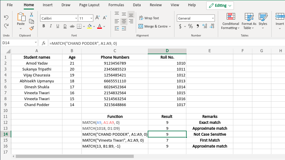
Output Screenshot

Like Article

Save Article

Источник

Product	Price
Apples	$1.00
Oranges	$0.75
Bananas	$0.50

Syntax

Example

Need more help?

Match type information

Exact match

Approximate match

Wildcard match

INDEX and MATCH

Case-sensitive match

Notes

Description

Syntax

Parameters or Arguments

Returns

Note

Applies To

Type of Function

Example (as Worksheet Function)

Frequently Asked Questions

How to Use the MATCH function in Excel: Step-by-Step

How to use the MATCH function

Approximate match types

Match type (1)

Match type (-1)

Other MATCH formula examples

That’s it – Now what

Other resources

Frequently asked question

What is Match Function in Excel?

Key Highlights

Syntax of MATCH function in Excel

How to Use Match Function in Excel?

#1 Finding The Exact Match

#2 Finding Partial Match using Wildcard Character

#3 Using INDEX and MATCH Function Together

Things to Remember

Frequently Asked Questions (FAQs)

Recommended Articles

Table of contents

The Syntax of the MATCH Excel Function

How to use the MATCH Function in Excel? (With Examples)

Example #1–Exact Match

Example #2–Approximate Match

Example #3–Wildcard Character (Partial Match)

Example 4–INDEX MATCH

The Properties of the MATCH Excel Function

Frequently Asked Questions

Recommended Articles

Excel Match Function Definition:

Syntax of Match Formula:

Few Important things about Match Formula:

Example of Match Formula in Excel:

WildCard Operators in Match Function: