
Содержание
- Locate and reset the last cell on a worksheet
- Locate the last cell that contains data or formatting on a worksheet
- Clear all formatting between the last cell and the data
- Need more help?
- Get value of last non-empty cell
- Related functions
- Summary
- Generic formula
- Explanation
- Get corresponding value
- Dealing with errors
- Last numeric value
- Last non-blank, non-zero value
- Position of the last value
- How to find the last used cell (row or column) in Excel
- The UsedRange object
- Find the last cell that contains data in a row or column
- Find the last cell that contains data in an Excel range
- Find the last cell that contains a formula
- Find the last cell that contains data and has a comment
- Find the last cell that is empty but contains a comment
- Find the last cell that is empty but formatted
- Find the last hidden cell in Excel
- What about performance when dealing with large worksheets or ranges?
- Available downloads:
- VBA Tutorial: Find the Last Row, Column, or Cell on a Sheet
- Video: 3 Part Series How to Find the Last Cell with VBA
- Download the Excel file that contains the code:
- Finding the Last Cell is All About the Data
- #1 – The Range.End() Method
- Range.End VBA Code Example
- Pros of Range.End
- Cons of Range.End
- #2 – The Range.Find() Method
- Range.Find Code Example
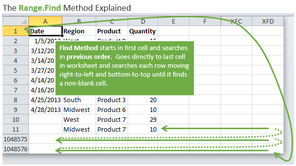
- The Range.Find Method Explained
- Pros of Range.Find
- Cons of Range.Find
- Macro Recorder to the Rescue!
- Use a Custom Function for the Find Method
- #3 – Range.SpecialCells(xlCellTypeLastCell)
- SpecialCells(xlCellTypeLastCell) Code Example
- Pros of Range.SpecialCells
- Cons of Range.SpecialCells
- Other Methods for Finding the Last Cell
Locate and reset the last cell on a worksheet
When you save a workbook, Excel stores only the part of each worksheet that contains data or formatting. Empty cells may contain formatting that causes the last cell in a row or column to fall outside of the range of cells that contains data. This causes the file size of the workbook to be larger than necessary and may result in more printed pages when you print the worksheet or workbook.
To avoid these issues, you can locate the last cell that contains data or formatting on a worksheet, and then reset that last cell by clearing all of the formatting that may be applied in empty rows or columns between the data and the last cell.
Locate the last cell that contains data or formatting on a worksheet
To locate the last cell that contains data or formatting, click anywhere in the worksheet, and then press CTRL+END.
Note: To select the very last cell in a row or column, press END, and then press the RIGHT ARROW key or the DOWN ARROW key.
Clear all formatting between the last cell and the data
Do one of the following:
To select all columns to the right of the last column that contains data, click the first column heading, hold down CTRL, and then click the column headings of the columns that you want to select.
Tip: You can also click the first column heading, and then press CTRL+SHIFT+END.
To select all rows below the last row that contains data, click the first row heading, hold down CTRL, and then click the row headings of the rows that you want to select.
Tip: You can also click the first row heading, and then press CTRL+SHIFT+END.
On the Home tab, in the Editing group, click the arrow next to the Clear button  , and then click Clear All.
Save the worksheet.
Close the worksheet.
When you open the workbook again, the last cell of the data should be the last cell on the worksheet.
Need more help?
You can always ask an expert in the Excel Tech Community or get support in the Answers community.
Источник
Get value of last non-empty cell
![]()
Summary
To find the value of the last non-empty cell in a row or column, even when data may contain empty cells, you can use the LOOKUP function with an array operation. The formula in F6 is:
The result is the last value in column B. The data in B:B can contain empty cells (i.e. gaps) and does not need to be sorted.
Note: This is an array formula. But because LOOKUP can handle the array operation natively, the formula does not need to be entered with Control + Shift + Enter, even in older versions of Excel.
Generic formula
Explanation
In this example, the goal is to get the last value in column B, even when data may contain empty cells. This is one of those puzzles that comes up frequently in Excel, because the answer is not obvious. One way to do it is with the LOOKUP function, which can handle array operations natively and always assumes an approximate match. This makes the formula surprisingly simple and compact:
Working from the inside out, we use a logical expression to test for empty cells in column B:
The range B:B is a full column reference to every cell in column B. The key advantage of a full column reference is that it remains unaffected when rows are deleted or added.
Note: Excel is generally smart about evaluating formulas that use full column references, but you should take care to manage the used range. In this case, because we create a «virtual column» of over 1 million rows with the expression B:B<>«», the used range likely doesn’t matter as much, but the formula is definitely much slower than the same formula with fixed ranges. If you notice performance problems, try limiting the range. For example: =LOOKUP(2,1/(B1:B100<>«»),B1:B100)
The logical operator <> means not equal to, and «» means empty string, so this expression means column B is not empty. The result is an array of TRUE and FALSE values, where TRUE represents cells that are not empty and FALSE represents cells that are empty. This array begins like this:
Next, we divide the number 1 by the array. The math operation automatically coerces TRUE to 1 and FALSE to 0, so we have:
Since dividing by zero generates an error, the result is an array composed of 1s and #DIV/0 errors:
This array becomes the lookup_array argument in LOOKUP. Notice the 1s represent non-empty cells, and errors represent empty cells.
The lookup_value is given as the number 2. We are using 2 as a lookup value to force LOOKUP to scan to the end of the data. LOOKUP automatically ignore errors, so LOOKUP will scan through the 1s looking for a 2 that will never be found. When it reaches the end of the array, it will «step back» to the last 1, which corresponds to the last non-empty cell.
Finally, LOOKUP returns the corresponding value in result_vector (given as B:B), so the final result is: June 30, 2020.
The key to understanding this formula is to recognize that the lookup_value of 2 is deliberately larger than any values that will appear in the lookup_vector. When lookup_value can’t be found, LOOKUP will match the next smallest value that is not an error: the last 1 in the array. This works because LOOKUP assumes that values in lookup_vector are sorted in ascending order and always performs an approximate match. When LOOKUP can’t find a match, it will match the next smallest value.
Get corresponding value
You can easily adapt the lookup formula to return a corresponding value. For example, to get the price associated with the last value in column B, the formula in F7 is:
The only difference is that the result_vector argument has been supplied as C:C.
Dealing with errors
If the last non-empty cell contains an error, the error will be ignored. If you want to return an error that appears last in a range you can adjust the formula to use the ISBLANK and NOT functions like this:
Last numeric value
To get the last numeric value, you can add the ISNUMBER function like this:
Last non-blank, non-zero value
To check that the last value is not blank and not zero, you can adapt the formula with Boolean logic like this:
If you notice performance problems, limit the range (i.e. use B1:B100, B1:B1000, instead of B:B).
Position of the last value
To get the row number of the last value, you can use a formula like this:
We use the ROW function to feed row numbers for column B to LOOKUP as the result_vector to get the row number for the last match.
Источник
How to find the last used cell (row or column) in Excel
I have encountered many spreadsheets. Some have been quite elegant. Most were Spartan yet useful. And not-insignificant number were downright dreadful and incomprehensible. The elegant ones are delight to code against. They have structure and order. The dreadful ones are difficult to code against due to their unpredictable structure. Yet, these ugly spreadsheets are the very ones that test our mettle as Excel add-in developers.
I discuss these spreadsheet “profiles” because, today, I want to show some strategies for finding the last used cell in an Excel worksheet or range. Given this post belongs to the Beginning Excel Development series… I will keep it clean and work with a spreadsheet that looks just like this:
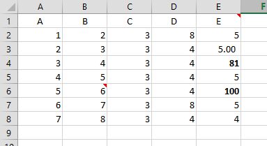
I went ahead and named this range “Sample”. I will refer to it throughout the code sample. It’s Spartan… but it is useful for today’s topic.
So, what do I mean by “last used cell”? I mean the last cell in a row or column that is used in one way or another. Meaning, it isn’t empty. It has a value, a formula, formatting, a comment, etc.
Some of you out there are already saying something like, “oh, oh, I know, I know… use the UsedRange property!”
Let’s consider it.
The UsedRange object
Taking a quick look at the MSDN reference material, UsedRange is a property of the Worksheet object. If you access it ask it to tell you its secrets, it will give you a Range object. This range will contain all the cells in the worksheet that have ever contained a value.
This means if a cell doesn’t contain a value now but did a few moments ago, UsedRange will gladly serve it up to you. It will keep this secret to itself and leave it to you to read the documentation. Thus, UsedRange can be unpredictable. Some developers go as far as to call it unreliable.
Fine, so what are some reliable methods for finding the last used cell in an Excel worksheet or a range? It depends on what you mean by the last cell? The following code sample show my ideas for how to tackle the following scenarios:
I like to take these things one-at-a-time.
Find the last cell that contains data in a row or column
![]()
When I say “contains data”, I mean the cell does not contain an empty string. It has something in it that is visible to the user. To a user, an empty string in a cell is an empty cell.
These are words to live by.
We’ll start simple, with a procedure named MoveToLastCellWithData. All it does is mimic the CTL+ARROW keyboard combination in Excel.
The procedure accepts an XlDirection parameter and then moves the cell selection in that direction. Below is how it can be utilized in a button click event.
Here, I create a range reference to the active cell. I then pass it on to MoveToLastCellWithData so that good things will happen.
Find the last cell that contains data in an Excel range
For the few samples, I want to utilize the SpecialCells collection. This collection resides under the Range object and lets you reference several types of special cells. I decided to create procedure that will let me pass a range along with the type of special cells I want. The procedures assumes I am asking it to tell me (by way of selecting it) which cell in the range is the last of this type.
Here is MoveToLastCell.
The method access the special cells and stuffs them into a range (cells). With some tricky math, it then selects that last cell.
Here is how to call it and tell it to find the last cell that contains data in the Sample range:
Find the last cell that contains a formula
And here is how to make the same call but find the last cell containing an Excel formula.
Find the last cell that contains data and has a comment
One last example with MoveToLastCell. This one finds the last cell that has data and a comment.
How about that, huh?
Find the last cell that is empty but contains a comment
Not impressed, let’s look at other empty cells. How about an empty cell that contains a comment? The MoveToLastEmptyCellbyType is the procedure we need. It is meant to do for empty cells what MoveToLastCell does for data-filled cells.
This should look familiar but the difference is we need to loop through the cells to check for the existence of a VBNullString or VBEmpty value. If we find it, we reference the cell and keep looping. Eventually the loop runs out and the last cell referenced is the last cell we are looking for.
A call to MoveToLastEmptyCellbyType looks like these two examples.
Find the last cell that is empty but formatted
Because we are friends, I’ll admit that this one was a slight pain to figure out and implementing it in an Excel solution will be highly variable. I chose to keep it very simple by only searching for cells containing bold formatting. LastEmptyButFormattedCell begins by setting find format to bold. It then references the Sample range then starts a search using the find format.
I want to point a few things:
- I coded this much like I would a VBA procedure.
- The loop will run forever if not for the check of exitLoop. I did it this way because of point #1.
- After referencing the sample range, the code moves the selection to the first cell (i.e. top-right) in the range. This is key because…
- The search’s direction is xlPrevious (i.e. backwards).
- After the first search, I store the address of the first cell. If we return to this cell in subsequent loops, we know we didn’t find any empty but formatted cells. So we need to exit the loop.
- If we find a cell that matches the search, we need to check its value for an empty string.
- If we find one, we select it and end the procedure. If we don’t fine one, we tell the user.
There might be a more elegant way to achieve the same thing. But this one tests out.
Finding the visible cells is easy using the SpecialCells and the MoveToLastCell method above:
But finding hidden cells is a different matter because no SpecialCell constant exists for hidden cells. Instead, we need to rummage around the sample range and consider the row and column of each cell. If either the row or the column is hidden, then we now that cell is hidden.
The ShowLastHiddenCell procedure loops through all cells. If any cells were hidden, it will show the address of the very last hidden cell it encountered.
What about performance when dealing with large worksheets or ranges?
This is always a limiting factor. I intentionally used a sample named range to keep from searching every cell in a worksheet. The more cells I’m searching the slower my add-in will perform. Thus, you need to implement strategies to ensure you are working only with a range of cells that makes sense for your scenario. If need to scan the entire worksheet, so be it… just display a “working on it” icon of your choosing so your user knows you are, uh, working on it.
It sure would be easier if the Excel object model allowed us to do this in straight-forward manner. But, if Microsoft did that, what would we do with ourselves?
Available downloads:
This sample Excel add-in was developed using Add-in Express for Office and .net:
Источник
VBA Tutorial: Find the Last Row, Column, or Cell on a Sheet
Bottom line: Learn how to find the last row, column, or cell in a worksheet using three different VBA methods. The method used depends on the layout of your data, and if the sheet contains blank cells.
Skill level: Intermediate
Video: 3 Part Series How to Find the Last Cell with VBA
Video best viewed in full screen HD
Download the Excel file that contains the code:
Jump to the Code Examples on this page:
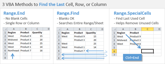
Finding the Last Cell is All About the Data
Finding the last used row, column, or cell is one very common task when writing macros and VBA applications. Like anything in Excel and VBA, there are many different ways to accomplish this.
Choosing the right method mostly depends on what your data looks like.
In this article I explain three different VBA methods of the Range object that we can use to find the last cell in a worksheet. Each of these methods has pros and cons, and some look scarier than others. 🙂
But understanding how each method works will help you know when to use them, and why.
#1 – The Range.End() Method
The Range.End method is very similar to pressing the Ctrl+Arrow Key keyboard shortcut. In VBA we can use this method to find the last non-blank cell in a single row or column.
![]()
Range.End VBA Code Example
To find the last used row in a column, this technique starts at the last cell in the column and goes up (xlUp) until it finds the first non-blank cell.
The Rows.Count statement returns a count of all the rows in the worksheet. Therefore, we are basically specifying the last cell in column A of the sheet (cell A1048567), and going up until we find the first non-blank cell.
It works the same with finding the last column. It starts at the last column in a row, then goes to the left until the last non-blank cell is found in the column. Columns.Count returns the total number of columns in the sheet. So we start at the last column and go left.
The argument for the End method specifies which direction to go. The options are: xlDown, xlUp, xlToLeft, xlToRight.
Pros of Range.End
- Range.End is simple to use and understand since it works the same way as the Ctrl+Arrow Key shortcuts.
- Can be used to find the first blank cell, or the last non-blank cell in a single row or column.
Cons of Range.End
- Range.End only works on a single row or column. If you have a range of data that contains blanks in the last row or column, then it may be difficult to determine which row or column to perform the method on.
- If you want to find the last used cell then you have to evaluate at least two statements. One to find the last row and one to find the last column. You can then combine these to reference the last cell.
Here are the help articles for Range.End
#2 – The Range.Find() Method
![]()
The Range.Find method is my preferred way to find the last row, column, or cell. It is the most versatile, but also the scariest looking. 🙂
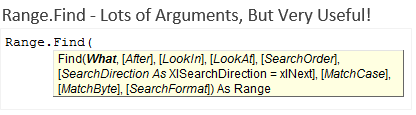
Range.Find has a lot of arguments, but don’t let this scare you. Once you know what they do you can use Range.Find for a lot of things in VBA.
Range.Find is basically the way to program the Find menu in Excel. It does the same thing, and most of the arguments of Range.Find are the options on the Find menu.
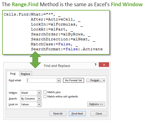
Range.Find Code Example
The following is the code to find the last non-blank row.
The Range.Find Method Explained
The Find method is looking for the first non-blank cell (“*”). The asterisk represents a wildcard character that looks for any text or numbers in the cell.
Starting in cell A1, it moves backwards (xlPrevious) and actually starts it’s search in the very last cell in the worksheet. It then moves right-to-left (xlByRows) and loops up through each row until it finds a non-blank cell. When a non-blank is found it stops and returns the row number.
Here is a detailed explanation for each argument.
- What:=”*” – The asterisk is a wildcard character that finds any text or number in the cell. It’s basically the same as searching for a non-blank cell.
- After:=Range(“A1”) – Start the search after cell A1, the first cell in the sheet. This means that A1 will NOT be searched. It will start the search after A1 and the next cell it searches depends on the SearchOrder and SearchDirection. This argument can be changed to start in a different cell, just remember that the search actually starts in the cell after the one specified.
- LookAt:=xlPart – This is going to look at any part of the text inside the cell. The other option is xlWhole, which would try to match the entire cell contents.
- LookIn:=xlFormulas – This tells Find to look in the formulas, and it is an important argument. The other option is xlValues, which would only search the values. If you have formulas that are returning blanks (=IF(A2>5,”Ok”,””) then you might want to consider this a non-blank cell. Specifying the LookIn as xlFormulas will consider this formula as non-blank, even if the value returned is blank.
- SearchOrder:=xlByRows – This tells Find to search through each entire row before moving on to the next. The direction is searches left-to-right or right-to-left depends on the SearchDirection argument. The other option here is xlByColumns, which is used when finding the last column.
- SearchDirection:=xlPrevious – This specifies which direction to search. xlPrevious means it will search from right-to-left or bottom-to-top. The other option is xlNext, which moves in the opposite direction.
- MatchCase:=False – This tells Find not to consider upper or lower case letters. Setting it to True would consider the case. This argument isn’t necessary for this scenario.
Ok, I know that’s a lot to read, but hopefully you will have a better understanding of how to use these arguments to find anything in a worksheet.
Pros of Range.Find
- Range.Find searches an entire range for the last non-blank row or column. It is NOT limited to a single row or column.
- The last row in a data set can contain blanks and Range.Find will still find the last row.
- The arguments can be used to search in different directions and for specific values, not just blank cells.
Cons of Range.Find
- It’s ugly. The method contains 9 arguments. Although only one of these arguments (What) is required, you should get in a habit of using at least the first 7 arguments. Otherwise, the Range.Find method will default to your last used settings in the Find window. This is important. If you don’t specify the optional arguments for LookAt, LookIn, and SearchOrder then the Find method will use whatever options you used last in Excel’s Find Window.
- Finding the last cell requires two statements. One to find the last row and one to find the last column. You then have to combine these to find the last cell.
Macro Recorder to the Rescue!
Range.Find is still my preferred method for finding the last cell because of it’s versatility. But it is a lot to type and remember. Fortunately, you don’t have to.
You can use the macro recorder to quickly create the code with all the arguments.
- Start the macro recorder
- Press Ctrl+F
- Then press the Find Next button
The code for the Find method with all the arguments will be generated by the macro recorder.
Use a Custom Function for the Find Method
You can also use a custom function (UDF) for the find method. Ron de Bruin’s Last Function is a perfect example. You can copy that function into any VBA project or code module, and use it to return the last row, column, or cell.
I also have a similar function in the example workbook. My function just has additional arguments to reference the worksheet and range to search in.
Here are the help articles for Range.Find
#3 – Range.SpecialCells(xlCellTypeLastCell)
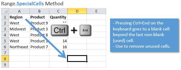
The SpecialCells method does the same thing as pressing the Ctrl+End keyboard shortcut, and selects the last used cell on the sheet.
SpecialCells(xlCellTypeLastCell) Code Example
It’s actually the easiest way to find the last used cell. However, this method is finding the last used cell, which can be different than the last non-blank cell.
Often times you will hit Ctrl+End on the keyboard and be taken to some cell way down at the end of the sheet that is definitely not used. This can occur for a number of reasons. One common reason is the formatting properties for that cell have been changed. Simply changing the font size or fill color of a cell will flag it as a used cell.
Pros of Range.SpecialCells
- You can use this method to find “used” rows and columns at the end of a worksheet and delete them. Comparing the result of Range.SpecialCells with the result of the Range.Find for non-blanks can allow you to quickly determine if any unused rows or columns exist on the sheet.
- Deleting unused rows/columns can reduce file size and make your scroll bar bigger.
Cons of Range.SpecialCells
- Excel only resets the last cell when the workbook is saved. So if the user or macro deletes the contents of some cells, then this method will not find the true last cell until after the file is saved.
- It finds the last used cell and NOT the last non-blank cell.
Other Methods for Finding the Last Cell
Well, that should cover the basics of finding the last used or non-blank cell in a worksheet. If you sheet contains objects (tables, charts, pivot tables, slicers, etc.) then you might need to use other methods to find the last cell. I will explain those techniques in a separate post.
Please leave a comment below if you have any questions, or are still having trouble finding the last cell. I’ll be happy to help! 🙂
Источник
Excel for Microsoft 365 Excel 2021 Excel 2019 Excel 2016 Excel 2013 Excel 2010 Excel 2007 More…Less
When you save a workbook, Excel stores only the part of each worksheet that contains data or formatting. Empty cells may contain formatting that causes the last cell in a row or column to fall outside of the range of cells that contains data. This causes the file size of the workbook to be larger than necessary and may result in more printed pages when you print the worksheet or workbook.
To avoid these issues, you can locate the last cell that contains data or formatting on a worksheet, and then reset that last cell by clearing all of the formatting that may be applied in empty rows or columns between the data and the last cell.
Locate the last cell that contains data or formatting on a worksheet
-
To locate the last cell that contains data or formatting, click anywhere in the worksheet, and then press CTRL+END.
Note: To select the very last cell in a row or column, press END, and then press the RIGHT ARROW key or the DOWN ARROW key.
Clear all formatting between the last cell and the data
-
Do one of the following:
-
To select all columns to the right of the last column that contains data, click the first column heading, hold down CTRL, and then click the column headings of the columns that you want to select.
Tip: You can also click the first column heading, and then press CTRL+SHIFT+END.
-
To select all rows below the last row that contains data, click the first row heading, hold down CTRL, and then click the row headings of the rows that you want to select.
Tip: You can also click the first row heading, and then press CTRL+SHIFT+END.
-
-
On the Home tab, in the Editing group, click the arrow next to the Clear button
 , and then click Clear All.
 -
Save the worksheet.
-
Close the worksheet.
When you open the workbook again, the last cell of the data should be the last cell on the worksheet.
Need more help?
You can always ask an expert in the Excel Tech Community or get support in the Answers community.
Top of Page
Need more help?
Want more options?
Explore subscription benefits, browse training courses, learn how to secure your device, and more.
Communities help you ask and answer questions, give feedback, and hear from experts with rich knowledge.

Posted on Friday, December 6th, 2013 at 9:26 am by .
I have encountered many spreadsheets. Some have been quite elegant. Most were Spartan yet useful. And not-insignificant number were downright dreadful and incomprehensible. The elegant ones are delight to code against. They have structure and order. The dreadful ones are difficult to code against due to their unpredictable structure. Yet, these ugly spreadsheets are the very ones that test our mettle as Excel add-in developers.
I discuss these spreadsheet “profiles” because, today, I want to show some strategies for finding the last used cell in an Excel worksheet or range. Given this post belongs to the Beginning Excel Development series… I will keep it clean and work with a spreadsheet that looks just like this:
I went ahead and named this range “Sample”. I will refer to it throughout the code sample. It’s Spartan… but it is useful for today’s topic.
So, what do I mean by “last used cell”? I mean the last cell in a row or column that is used in one way or another. Meaning, it isn’t empty. It has a value, a formula, formatting, a comment, etc.
Some of you out there are already saying something like, “oh, oh, I know, I know… use the UsedRange property!”
Let’s consider it.
The UsedRange object
Taking a quick look at the MSDN reference material, UsedRange is a property of the Worksheet object. If you access it ask it to tell you its secrets, it will give you a Range object. This range will contain all the cells in the worksheet that have ever contained a value.
This means if a cell doesn’t contain a value now but did a few moments ago, UsedRange will gladly serve it up to you. It will keep this secret to itself and leave it to you to read the documentation. Thus, UsedRange can be unpredictable. Some developers go as far as to call it unreliable.
Fine, so what are some reliable methods for finding the last used cell in an Excel worksheet or a range? It depends on what you mean by the last cell? The following code sample show my ideas for how to tackle the following scenarios:
- Find the last cell that contains data in a row or column
- Find the last cell that contains data in a range
- Find the last cell that contains a formula
- Find the last cell that contains data and has a comment
- Find the last cell that is empty but contains a comment
- Find the last cell that is empty but formatted
- Find the last hidden cell
I like to take these things one-at-a-time.
Find the last cell that contains data in a row or column

When I say “contains data”, I mean the cell does not contain an empty string. It has something in it that is visible to the user. To a user, an empty string in a cell is an empty cell.
These are words to live by.
We’ll start simple, with a procedure named MoveToLastCellWithData. All it does is mimic the CTL+ARROW keyboard combination in Excel.
Private Sub MoveToLastCellWithData(currentCell As Excel.Range, direction As Excel.XlDirection)
    currentCell.End(direction).Select()
End Sub
The procedure accepts an XlDirection parameter and then moves the cell selection in that direction. Below is how it can be utilized in a button click event.
Private Sub MoveToRight_OnClick(sender As Object, _
    control As IRibbonControl, pressed As Boolean) Handles MoveToRight.OnClick

    Dim rg As Excel.Range = ExcelApp.ActiveCell
    MoveToLastCellWithData(rg, Excel.XlDirection.xlToRight)
    Marshal.ReleaseComObject(rg)
End Sub
Here, I create a range reference to the active cell. I then pass it on to MoveToLastCellWithData so that good things will happen.
Find the last cell that contains data in an Excel range
For the few samples, I want to utilize the SpecialCells collection. This collection resides under the Range object and lets you reference several types of special cells. I decided to create procedure that will let me pass a range along with the type of special cells I want. The procedures assumes I am asking it to tell me (by way of selecting it) which cell in the range is the last of this type.
Here is MoveToLastCell.
Private Sub MoveToLastCell(cellType As Excel.XlCellType, _
    sheet As Excel.Worksheet, rangeName As String)

    Dim cells As Object = Nothing
    Dim lastCell As Excel.Range = Nothing
    Try
        cells = sheet.Range(rangeName).SpecialCells(cellType).Areas

        lastCell = cells(cells.Count)
        lastCell.Select()

    Catch
    End Try

    If lastCell IsNot Nothing Then Marshal.ReleaseComObject(lastCell)
    If cells IsNot Nothing Then Marshal.ReleaseComObject(cells)
End Sub
The method access the special cells and stuffs them into a range (cells). With some tricky math, it then selects that last cell.
Here is how to call it and tell it to find the last cell that contains data in the Sample range:
MoveToLastCell(Excel.XlCellType.xlCellTypeLastCell, ExcelApp.ActiveSheet, "Sample")
Boom!
Find the last cell that contains a formula
And here is how to make the same call but find the last cell containing an Excel formula.
MoveToLastCell(Excel.XlCellType.xlCellTypeFormulas, ExcelApp.ActiveSheet, "Sample")
Pretty cool, eh?
Find the last cell that contains data and has a comment
One last example with MoveToLastCell. This one finds the last cell that has data and a comment.
MoveToLastCell(Excel.XlCellType.xlCellTypeComments, ExcelApp.ActiveSheet, "Sample")
How about that, huh?
Find the last cell that is empty but contains a comment
Not impressed, let’s look at other empty cells. How about an empty cell that contains a comment? The MoveToLastEmptyCellbyType is the procedure we need. It is meant to do for empty cells what MoveToLastCell does for data-filled cells.
Private Sub MoveToLastEmptyCellByType(cellType As Excel.XlCellType, _
    sheet As Excel.Worksheet, rangeName As String)

    Dim cells As Object
    cells = sheet.Range(rangeName).SpecialCells(cellType).Areas

    Dim lastCell As Excel.Range = Nothing

    For i = 1 To cells.Count
        Dim cell As Excel.Range = cells(i)
        If cell.Value2 = vbNullString or VBEmpty Then
            lastCell = cell
            lastCell.Select()
        End If
        Marshal.ReleaseComObject(cell)
    Next

    'Check and return the last cell if still Nothing
    If lastCell Is Nothing Then
        lastCell = cells(cells.Count)
    End If
    If lastCell isnot Nothing then Marshal.ReleaseComObject(lastCell)
    If cells IsNot Nothing Then Marshal.ReleaseComObject(cells)
End Sub
This should look familiar but the difference is we need to loop through the cells to check for the existence of a VBNullString or VBEmpty value. If we find it, we reference the cell and keep looping. Eventually the loop runs out and the last cell referenced is the last cell we are looking for.
A call to MoveToLastEmptyCellbyType looks like these two examples.
MoveToLastEmptyCellbyType(Excel.XlCellType.xlCellTypeComments, ExcelApp.ActiveSheet, "Sample")
MoveToLastEmptyCellbyType(Excel.XlCellType.xlCellTypeFormulas, ExcelApp.ActiveSheet, "Sample")
Find the last cell that is empty but formatted
Because we are friends, I’ll admit that this one was a slight pain to figure out and implementing it in an Excel solution will be highly variable. I chose to keep it very simple by only searching for cells containing bold formatting. LastEmptyButFormattedCell begins by setting find format to bold. It then references the Sample range then starts a search using the find format.
Private Sub LastEmptyButFormattedCell()
    ExcelApp.FindFormat.Font.FontStyle = "Bold"

    Dim sheet As Excel.Worksheet = ExcelApp.ActiveSheet
    Dim found As Object = Nothing
    Dim loopCount As Integer = 0
    Dim firstCellAddress As String = ""
    Dim exitLoop As Boolean = False
    Dim emptyFound As Boolean = False

    With sheet.Range("Sample")
        'Select the range...
        .Select()
        'Ensure we are in the top-right cell
        .Cells(1, 1).Activate()

        Do
            'Do we need to exit the DO...LOOP?
            If exitLoop Then Exit Do

            'Peform a search
            found = .Find("", ExcelApp.ActiveCell, Excel.XlFindLookIn.xlValues, _
                Excel.XlLookAt.xlPart, Excel.XlSearchOrder.xlByRows, _
                Excel.XlSearchDirection.xlPrevious, MatchCase:=False, _
                SearchFormat:=True)

            'Check that we found a cell and activate it
            If Not found Is Nothing Then found.Activate()

            Select Case loopCount
                'The first time through the loop
                Case 0
                    'grab the address of this initial cell.
                    firstCellAddress = found.Address
                    loopCount = 1
                Case 1 'All subsequent loops
                    'if we are back at the first cell,
                    'we need to get out of the loop.
                    If firstCellAddress = found.Address Then
                        exitLoop = True
                    End If
                Case Else
            End Select

            If found.Value = vbEmpty Then
                'We found a formatted cell with an empty value...time to leave.
                emptyFound = True
                exitLoop = True
            End If
        Loop

        'We found, so select it to show the user.
        If emptyFound Then
            found.Select()
        Else
            MsgBox("No empty empty formatted cells exist.")
        End If
    End With

    If found IsNot Nothing Then Marshal.ReleaseComObject(found)
    Marshal.ReleaseComObject(sheet)
End Sub
I want to point a few things:
- I coded this much like I would a VBA procedure.
- The loop will run forever if not for the check of exitLoop. I did it this way because of point #1.
- After referencing the sample range, the code moves the selection to the first cell (i.e. top-right) in the range. This is key because…
- The search’s direction is xlPrevious (i.e. backwards).
- After the first search, I store the address of the first cell. If we return to this cell in subsequent loops, we know we didn’t find any empty but formatted cells. So we need to exit the loop.
- If we find a cell that matches the search, we need to check its value for an empty string.
- If we find one, we select it and end the procedure. If we don’t fine one, we tell the user.
There might be a more elegant way to achieve the same thing. But this one tests out.
Find the last hidden cell in Excel
Finding the visible cells is easy using the SpecialCells and the MoveToLastCell method above:
MoveToLastCell(Excel.XlCellType.xlCellTypeVisible, ExcelApp.ActiveSheet, "Sample")
But finding hidden cells is a different matter because no SpecialCell constant exists for hidden cells. Instead, we need to rummage around the sample range and consider the row and column of each cell. If either the row or the column is hidden, then we now that cell is hidden.
Private Sub ShowLastHiddenCell()
    Dim foundCells As Excel.Range
    Dim sheet As Excel.Worksheet = ExcelApp.ActiveSheet

    foundCells = sheet.Range("sample")

    If Not foundCells Is Nothing Then
        'Loop through the cells and find the last one in the range that is hidden.
        Dim lastCell As Excel.Range = Nothing
        Dim address As String = Nothing
        For i = 1 To foundCells.Count
            Dim cell As Excel.Range = foundCells(i)
            If cell.EntireColumn.Hidden = True Or cell.EntireRow.Hidden = True Then
                'You are forgiven for thinking you can check Cell.Hidden
                lastCell = cell
                address = lastCell.Address
            End If
            Marshal.ReleaseComObject(cell)
        Next

        'Check and return the last cell if still Nothing
        If lastCell Is Nothing Then
            MsgBox("No hidden cells found.")
        Else
            MsgBox("The last hidden cell resides in " & address)
        End If
    End If
  Marshal.ReleaseComObject(foundCells)
End Sub
The ShowLastHiddenCell procedure loops through all cells. If any cells were hidden, it will show the address of the very last hidden cell it encountered.
What about performance when dealing with large worksheets or ranges?
This is always a limiting factor. I intentionally used a sample named range to keep from searching every cell in a worksheet. The more cells I’m searching the slower my add-in will perform. Thus, you need to implement strategies to ensure you are working only with a range of cells that makes sense for your scenario. If need to scan the entire worksheet, so be it… just display a “working on it” icon of your choosing so your user knows you are, uh, working on it.
*****
It sure would be easier if the Excel object model allowed us to do this in straight-forward manner. But, if Microsoft did that, what would we do with ourselves?
Available downloads:
This sample Excel add-in was developed using Add-in Express for Office and .net:
Find Last Cell Excel Add-in (VB.NET)
You may also be interested in:
- Creating COM add-ins for Excel 2013 – 2007. Customizing Excel Ribbon
- Excel add-in development in Visual Studio
NOTE: I intend to make this a «one stop post» where you can use the Correct way to find the last row. This will also cover the best practices to follow when finding the last row. And hence I will keep on updating it whenever I come across a new scenario/information.
Unreliable ways of finding the last row
Some of the most common ways of finding last row which are highly unreliable and hence should never be used.
- UsedRange
- xlDown
- CountA
UsedRange should NEVER be used to find the last cell which has data. It is highly unreliable. Try this experiment.
Type something in cell A5. Now when you calculate the last row with any of the methods given below, it will give you 5. Now color the cell A10 red. If you now use the any of the below code, you will still get 5. If you use Usedrange.Rows.Count what do you get? It won’t be 5.
Here is a scenario to show how UsedRange works.

xlDown is equally unreliable.
Consider this code
lastrow = Range("A1").End(xlDown).Row
What would happen if there was only one cell (A1) which had data? You will end up reaching the last row in the worksheet! It’s like selecting cell A1 and then pressing End key and then pressing Down Arrow key. This will also give you unreliable results if there are blank cells in a range.
CountA is also unreliable because it will give you incorrect result if there are blank cells in between.
And hence one should avoid the use of UsedRange, xlDown and CountA to find the last cell.
Find Last Row in a Column
To find the last Row in Col E use this
With Sheets("Sheet1")
    LastRow = .Range("E" & .Rows.Count).End(xlUp).Row
End With
If you notice that we have a . before Rows.Count. We often chose to ignore that. See THIS question on the possible error that you may get. I always advise using . before Rows.Count and Columns.Count. That question is a classic scenario where the code will fail because the Rows.Count returns 65536 for Excel 2003 and earlier and 1048576 for Excel 2007 and later. Similarly Columns.Count returns 256 and 16384, respectively.
The above fact that Excel 2007+ has 1048576 rows also emphasizes on the fact that we should always declare the variable which will hold the row value as Long instead of Integer else you will get an Overflow error.
Note that this approach will skip any hidden rows. Looking back at my screenshot above for column A, if row 8 were hidden, this approach would return 5 instead of 8.
Find Last Row in a Sheet
To find the Effective last row in the sheet, use this. Notice the use of Application.WorksheetFunction.CountA(.Cells). This is required because if there are no cells with data in the worksheet then .Find will give you Run Time Error 91: Object Variable or With block variable not set
With Sheets("Sheet1")
    If Application.WorksheetFunction.CountA(.Cells) <> 0 Then
        lastrow = .Cells.Find(What:="*", _
                      After:=.Range("A1"), _
                      Lookat:=xlPart, _
                      LookIn:=xlFormulas, _
                      SearchOrder:=xlByRows, _
                      SearchDirection:=xlPrevious, _
                      MatchCase:=False).Row
    Else
        lastrow = 1
    End If
End With
Find Last Row in a Table (ListObject)
The same principles apply, for example to get the last row in the third column of a table:
Sub FindLastRowInExcelTableColAandB()
Dim lastRow As Long
Dim ws As Worksheet, tbl as ListObject
Set ws = Sheets("Sheet1")  'Modify as needed
'Assuming the name of the table is "Table1", modify as needed
Set tbl = ws.ListObjects("Table1")

With tbl.ListColumns(3).Range
    lastrow = .Find(What:="*", _
                After:=.Cells(1), _
                Lookat:=xlPart, _
                LookIn:=xlFormulas, _
                SearchOrder:=xlByRows, _
                SearchDirection:=xlPrevious, _
                MatchCase:=False).Row
End With

End Sub
The ADDRESS function creates a reference based on a given a row and column number. In this case, we want to get the last row and the last column used by the named range data (B5:D14).
To get the last row used, we use the ROW function together with the MAX function like this:
MAX(ROW(data))
Because data contains more than one row, ROW returns an array of row numbers:
{5;6;7;8;9;10;11;12;13;14}
This array goes directly to the MAX function, which returns the largest number:
MAX({5;6;7;8;9;10;11;12;13;14}) // returns 14
To get the last column, we use the COLUMN function in the same way:
MAX(COLUMN(data))
Since data contains three rows, COLUMN returns an array with three column numbers:
{2,3,4}
and the MAX function again returns the largest number:
MAX({2,3,4}) // returns 4
Both results are returned directly to the ADDRESS function, which constructs a reference to the cell at row 14, column 4:
=ADDRESS(14,4) // returns $D$14
If you want a relative address instead of an absolute reference, you can supply 4 for the third argument like this:
=ADDRESS(MAX(ROW(data)),MAX(COLUMN(data)),4) // returns D14
CELL function alternative
Although it’s not obvious, the INDEX function returns a reference, so we can use the CELL function with INDEX to get the address of the last cell in a range like this:
=CELL("address",INDEX(data,ROWS(data),COLUMNS(data)))
In this case, we use the INDEX function to get a reference to the last cell in the range, which we determine by passing total rows and total columns for the range data into INDEX. We get total rows with the ROWS function, and total columns with the COLUMNS function:
ROWS(data) // returns 10
COLUMNS(data) // returns 3
With the array provided as data, INDEX then returns a reference to cell D14:
INDEX(data,10,3) // returns reference to D14
We then use the CELL function with «address», to display the address.
Note: The CELL function is a volatile function which can cause performance problems in large or complex workbooks.