
Excel for Microsoft 365 Excel 2021 Excel 2019 Excel 2016 Excel 2013 Excel 2010 Excel 2007 More…Less
Let’s say you want to find out who has the the smallest error rate in a production run at a factory or the largest salary in your department. There are several ways to calculate the smallest or largest number in a range.
If the cells are in a contiguous row or column
-
Select a cell below or to the right of the numbers for which you want to find the smallest number.
-
On the Home tab, in the Editing group, click the arrow next to AutoSum
 , click Min (calculates the smallest) or Max (calculates the largest), and then press ENTER.
 , click Min (calculates the smallest) or Max (calculates the largest), and then press ENTER.
If the cells are not in a contiguous row or column
To do this task, use the MIN, MAX, SMALL, or LARGE functions.
Example
Copy the following data to a blank worksheet.
|
|
Need more help?
You can always ask an expert in the Excel Tech Community or get support in the Answers community.
See Also
LARGE
MAX
MIN
SMALL
Need more help?
Want more options?
Explore subscription benefits, browse training courses, learn how to secure your device, and more.
Communities help you ask and answer questions, give feedback, and hear from experts with rich knowledge.
largest.
MAX will return the largest value in a given list of arguments. From a given set of numeric values, it will return the highest value. Unlike MAXA function, the MAX function will count numbers but ignore empty cells, text, the logical values TRUE and FALSE, and text values.
Contents
- 1 What does max and min mean in Excel?
- 2 What is the max cell in Excel?
- 3 How do you find Max?
- 4 How do you do MIN and MAX in Excel?
- 5 How do you calculate Max in Excel?
- 6 What type of reference is a $4?
- 7 What is the function of max ()?
- 8 How do you find the maximum value in Excel?
- 9 How do I find the maximum name in Excel?
- 10 How do you find the maximum of a set of data?
- 11 What is maximum point?
- 12 What is the meaning of minimum and maximum?
- 13 How do you find max and min?
- 14 What type of cell reference is a $1?
- 15 What does $4 in Excel mean?
- 16 What are the 3 types of cell references in Excel?
- 17 What is Max in computer?
- 18 What is the syntax of Max?
- 19 How do you use Max and index in Excel?
- 20 How do you remove limits from Excel?
The MIN and MAX functions are just what the names imply. MIN will find the lowest number in a range, while MAX finds the largest number in a range.
What is the max cell in Excel?
32,767 characters
Worksheet and workbook specifications and limits
| Feature | Maximum limit |
|---|---|
| Column width | 255 characters |
| Row height | 409 points |
| Page breaks | 1,026 horizontal and vertical |
| Total number of characters that a cell can contain | 32,767 characters |
How do you find Max?
How to Determine Maximum Value
- If your equation is in the form ax2 + bx + c, you can find the maximum by using the equation:
- max = c – (b2 / 4a).
- The first step is to determine whether your equation gives a maximum or minimum.
- -x2 + 4x – 2.
- Since the term with the x2 is negative, you know there will be a maximum point.
How do you do MIN and MAX in Excel?
Calculate the smallest or largest number in a range
- Select a cell below or to the right of the numbers for which you want to find the smallest number.
- On the Home tab, in the Editing group, click the arrow next to AutoSum. , click Min (calculates the smallest) or Max (calculates the largest), and then press ENTER.
How do you calculate Max in Excel?
The second method is Autosum:
- Highlight the cells you want to find the largest number from.
- Select the Formulas tab.
- Click Autosum. Select Max from the drop down menu. Make sure the cell below the list of numbers you selected has a blank cell below it. This cell below the list is where the largest number will appear.
What type of reference is a $4?
absolute reference
At times, cell references need to stay static when formulas are copied. Copying formulas is the other major use of an absolute reference such as =$A$2+$A$4. The values in those references don’t change when you copy them.
What is the function of max ()?
The Microsoft Excel MAX function returns the largest value from the numbers provided. The MAX function is a built-in function in Excel that is categorized as a Statistical Function. It can be used as a worksheet function (WS) in Excel.
How do you find the maximum value in Excel?
To get the position of the maximum value in a range (i.e. a list, table, or row), you can use the MAX function together with the MATCH function. Which returns the number 4, representing the position in this list of the the most expensive property.
How do I find the maximum name in Excel?
Let us take an example:
- In cell D2, the formula would be.
- =INDEX(A2:A9,MATCH(MAX(B2:B9),B2:B9,0))
- Press enter on your keyboard.
- The function will return the player name who scored the highest number.
How do you find the maximum of a set of data?
The maximum and minimum also make an appearance alongside the first, second, and third quartiles in the composition of values comprising the five number summary for a data set. The minimum is the first number listed as it is the lowest, and the maximum is the last number listed because it is the highest.
What is maximum point?
maximum, In mathematics, a point at which a function’s value is greatest. If the value is greater than or equal to all other function values, it is an absolute maximum.In calculus, the derivative equals zero or does not exist at a function’s maximum point.
What is the meaning of minimum and maximum?
Minimum means the least you can do of something.Maximum means the most you can have of something. For example, if the maximum amount of oranges you can juggle is five, you cannot juggle more than five oranges. You can do the maximum or less.
How do you find max and min?
Finding max/min: There are two ways to find the absolute maximum/minimum value for f(x) = ax2 + bx + c: Put the quadratic in standard form f(x) = a(x − h)2 + k, and the absolute maximum/minimum value is k and it occurs at x = h. If a > 0, then the parabola opens up, and it is a minimum functional value of f.
What type of cell reference is a $1?
Summary of absolute cell reference uses:
| $A1 | Allows the row reference to change, but not the column reference. |
|---|---|
| A$1 | Allows the column reference to change, but not the row reference. |
| $A$1 | Allows neither the column nor the row reference to change. |
What does $4 in Excel mean?
read morecontains dollar signs attached to each letter or number in a reference, e.g., $B$4, Here if we mention a dollar sign before the column and row identifiers, it makes absolute or locks both the column and the row, i.e., where Cell reference remains constant even if it copied or dragged to another cell.
What are the 3 types of cell references in Excel?
Relative, Absolute and Mixed
A key element of a formula is the cell reference, and there are three types: Relative. Absolute. Mixed.
What is Max in computer?
Max is short for maximize. 2. Short for maximum, max is a Microsoft Excel and spreadsheet formula to find the maximum value in a range of cells.If these cells had the values 1,2,3,4,5,6,7,8,9, and 10, the result would return “10” since it’s the largest (maximum) value in all of the cells.
What is the syntax of Max?
The MAX function syntax has the following arguments: Number1, number2,Number1 is required, subsequent numbers are optional. 1 to 255 numbers for which you want to find the maximum value.
How do you use Max and index in Excel?
Return the Min or Max Value Using a Lookup in Excel – INDEX MATCH
- Type =INDEX(
- Select the column that contains the data you want to return, in this case the Site column.
- Type a comma to go to the next argument and then type MATCH(
- Now, type MAX(
How do you remove limits from Excel?
Select the cell you want to clear the restricted value, then click Data > Data Validation. See screenshot: 2. In the opening Data Validation dialog box, please click the Clear All button under the Settings tab, and then click the OK button.
Excel is an amazing program to store and analyze hundreds (if not thousands!) of numbers, but sorting through all of that data to find something specific can be painful. If you need to quickly find the most expensive item in your 2016 budget, for example, you can use the MAX formula or AutoSum to uncover that value in seconds.
Check out the video above or steps below to learn how.
There are two ways to determine the highest number on an Excel spreadsheet. The first method is using a formula.
First method:
- In a blank cell, type “=MAX(“
- Select the cells you want to find the largest number from.
- Close the formula with an ending parentheses.
- Hit enter and the largest number from your selection will populate in the cell.
The second method is Autosum:
- Highlight the cells you want to find the largest number from.
- Select the Formulas tab.
- Click Autosum.
- Select Max from the drop down menu.
- Make sure the cell below the list of numbers you selected has a blank cell below it. This cell below the list is where the largest number will appear.
- Select Max from the drop down menu.
Содержание
- How to find sum of largest N numbers in Excel
- SUM largest 2, 3, 5 or n numbers in a range
- Find sum of highest values with SUMPRODUCT
- How to sum many top numbers
- How to sum a variable number of largest values
- 1. Return the sum of n largest or all items
- 2. Show a custom message if not enough data
- Sum largest numbers in Excel 365 and Excel 2021
- How to sum top n values in Excel table
- How to Find the Largest Number in Excel
- Simplest Way How to Find the Largest Number in Excel
- How to Find the Largest Number in All Quarters
- MAX function in Excel: formula examples to find and highlight highest value
- Excel MAX function
- How to make a MAX formula in Excel
- 5 things to know about MAX function
- How to use MAX function in Excel – formula examples
- How to find max value in a group
- Find highest value in non-adjacent cells or ranges
- How to get max (latest) date in Excel
- MAX function in Excel with conditions
- Excel MAX IF formula
- Non-array MAX IF formula
- MAXIFS function
- Get max value ignoring zeros
- MAX IF
- MAXIFS
- Find highest value ignoring errors
- How to find absolute max value in Excel
- Return the maximum absolute value preserving the sign
- How to highlight max value in Excel
- Highlight highest number in a range
- Highlight max value in each row
- Excel MAX function not working
- MAX formula returns zero
- MAX formula returns #N/A, #VALUE or other error
How to find sum of largest N numbers in Excel
 by Alexander Frolov, updated on March 15, 2023
Six fast and reliable ways to do sum of the highest N values in Excel.
Adding things up is one of the most popular activities both in the business world and in everyday life. No wonder that Microsoft Excel comes equipped with a number of inbuild function such as, SUM, SUMIF, and SUMIFS.
In some situations, however, you may need to sum only specific numbers in a range, say top 3, 5, 10 or n. That might be a challenge because Excel has no inbuilt function for this. But as always, there is nothing that would prevent you from constructing your own formulas 🙂
SUM largest 2, 3, 5 or n numbers in a range
To sum top n numbers in a given array, the generic formula is:
For example, to get the sum of the largest 2 numbers in the range B2:B15, the formula is:
To sum 3 largest numbers:
To do a sum of 5 largest numbers:
The screenshot below shows all the formulas in action: 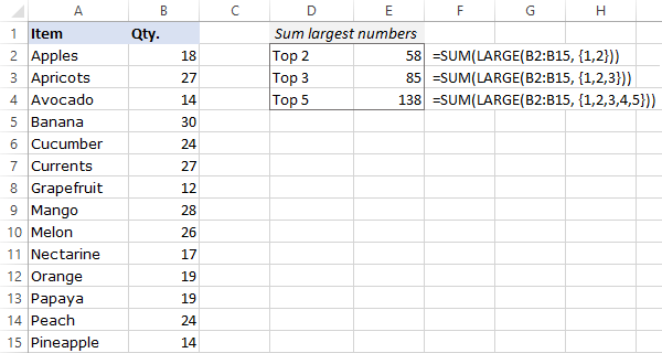
If the values’ ranks are input in predefined cells, you’d need to use a range reference for the k argument of LARGE. In this case, the solution must be entered as an array formula by pressing the Ctrl + Shift + Enter keys together. In Dynamic Array Excel (365 and 2021), this will also work as a regular formula.
For example, to get sum of the largest 3 adjacent or non-adjacent numbers whose ranks are in D2:D4, the formula is:
=SUM(LARGE(B2:B15, D2:D4)) 
Note. If there are two or more numbers that are tied for the last place, only the first number will be summed. For example, if the top 3 numbers are 10, 9 and 7, and the number 7 occurs in more than one cell, only the first occurrence of 7 will be added up.
How this formula works:
The core of the formula is the LARGE function that determines the Nth largest value in a given array. To get the top n values, an array constant such as <1,2,3>is supplied to the second argument:
As the result, LARGE returns the top 3 values in the range B2:B15, which are 30, 28 and 27.
The SUM function takes it from there, adds up the 3 numbers, and outputs the total:
Find sum of highest values with SUMPRODUCT
The SUMPRODUCT formula to return a sum of top N numbers is very much alike:
The beauty of SUMPRODUCT is that it works with array constants and cell references equally well. That is, regardless of whether you use <1,2,3>or D2:D4 for k inside LARGE, a regular formula will work nicely in all versions of Excel:
=SUMPRODUCT(LARGE(B2:B15, D2:D4)) 
How to sum many top numbers
If you are looking to add up the top 10 or 20 numbers in a range, listing their positions in an array constant manually may be quite tiresome. In this case, you can construct an array automatically by using the ROW and INDIRECT functions:
Please remember that the SUM + LARGE combination only works as an array formula in Excel 2019 and lower, so use the Ctrl + Shift + Enter shortcut to complete it correctly.
For instance, to sum 10 highest numbers in the range, use one of these formulas:
To make the formula more flexible, you can enter the number of items in some cell, say E2, and concatenate the cell reference inside INDIRECT:
In Excel 365 and Excel 2021, where the dynamic array behavior is native for all functions, both SUM and SUMPRODUCT work perfectly as regular formulas: 
How to sum a variable number of largest values
When there is insufficient data in the source range, i.e. n is larger than the total number of items, the formulas discussed above would result in an error: 
To handle this scenario, choose one of these solutions:
1. Return the sum of n largest or all items
With this approach, you output a sum of all existing values in case the specified n is larger than the total number of items in the range.
First, we get a count of all the numbers with the help of COUNT, and then use MIN to return either n or the count, whichever is smaller:
For our sample dataset, the formula takes this form:
=SUMPRODUCT(LARGE(B2:B15, ROW(INDIRECT(«1:»&MIN(E2, COUNT(B2:B15))))))
Because the specified n (15) is higher than the count (14), all the numbers in B2:B15 are summed: 
2. Show a custom message if not enough data
To make it explicitly clear that n exceeds the total number of items in the list, you can display a custom message using the IFERROR function:
=IFERROR(SUMPRODUCT(LARGE(B2:B15, ROW(INDIRECT(«1:»&E2)))), «Insufficient data») 
Sum largest numbers in Excel 365 and Excel 2021
Instead of constructing a cumbersome ROW + INDIRECT combination, the users of Excel 365 and Excel 2021 can employ the SEQUENCE function to generate a numeric array on the fly:
Because SEQUENCE is only available in the new Dynamic Array Excel where the array behavior is native for all the functions, you can safely replace SUMPRODUCT with a more concise SUM:
For example, to do sum of 5 largest numbers, use this compact and elegant formula:
=SUM(LARGE(B2:B15, SEQUENCE(E2))) 
How to sum top n values in Excel table
Excel tables come equipped with a number of awesome features, which let you get a sum of top N values in 4 easy steps:
- Convert a usual range to a table by pressing the Ctrl + T keys together.
- On the Table Design tab, in the Table Style Options group, enable the Total Row feature.
- In the header of the column containing your numbers, click the filter icon, and then click Number Filters >Top 10.

In a pop-up dialog box, specify how many top items to display: 
That’s it! Excel will immediately filter 10 top items (or whatever you choose) and calculate their total automatically.
To verify the result, let’s compare the table’s total with the result of our formula and make sure they are fully in line: 
These are the 6 effective ways to add up highest values in Excel. I thank you for reading and hope to see you on our blog next week!
Источник
How to Find the Largest Number in Excel
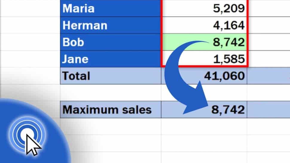
In the next couple of minutes, we’ll go through a quick guide on how to find the largest number in Excel. Thanks to these simple steps, you’ll be able to find out maximum sales for a certain period of time promptly.
See the video tutorial and transcription below:
The largest number of a group in Excel can be identified in more than one way. Today, we’ll cover just one, the simplest way, step by step, using this specific data set as an example.
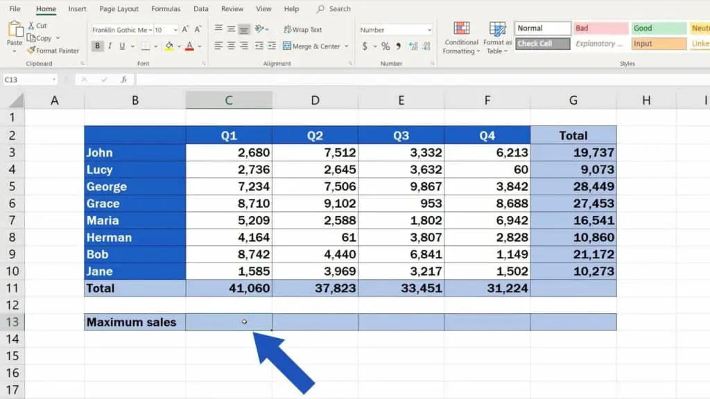
Simplest Way How to Find the Largest Number in Excel
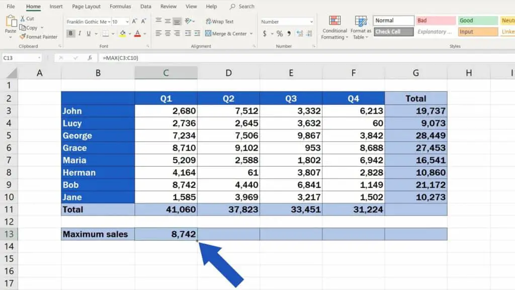
Set the pointer on the cell in which you want the largest number to appear. In this case, we’ll click on C13, where we want to display the maximum sales for Q1.
Go to ‘Home’ tab and look for the button ‘AutoSum’ in the group ‘Editing’. After clicking on the button, a drop-down menu will appear. 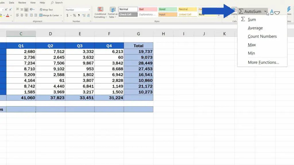
Since we’re looking for maximum sales, find and select the function ‘Max’. 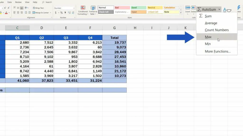
Excel will then prompt us to define the area in which we want to look for the maximum value, which is Q1. 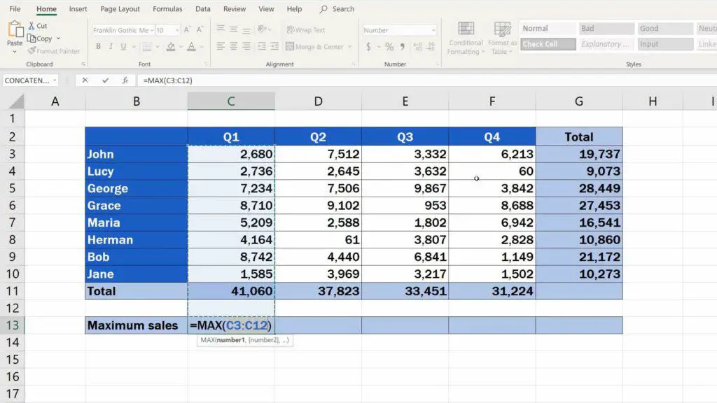
You can drag your mouse to select the cell range C3 to C10. 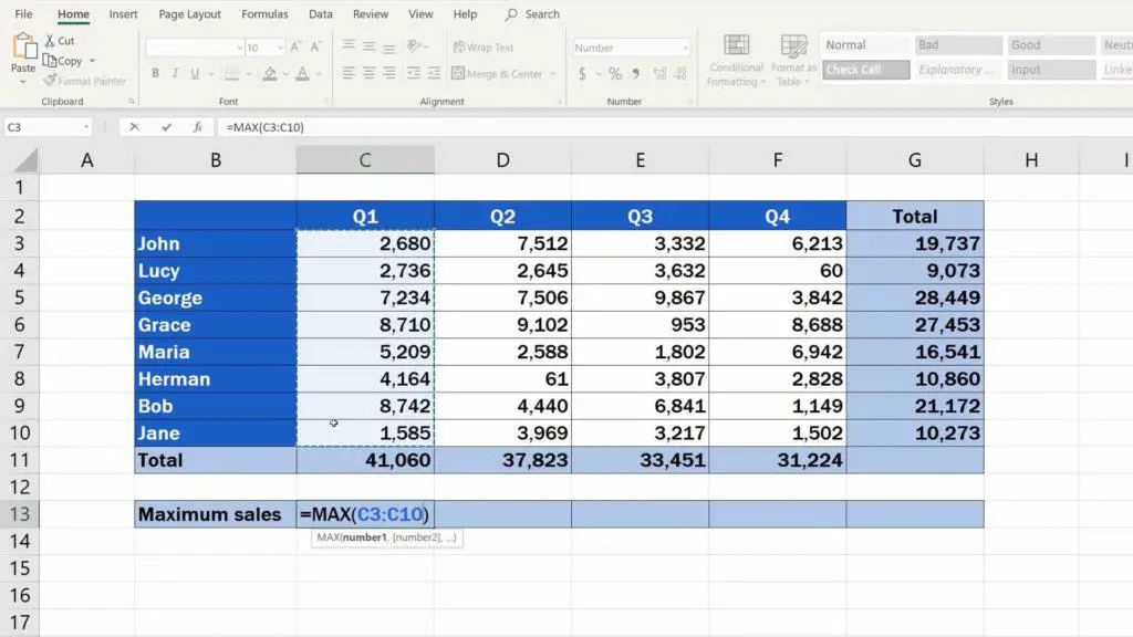
Now click on OK. Perfect! 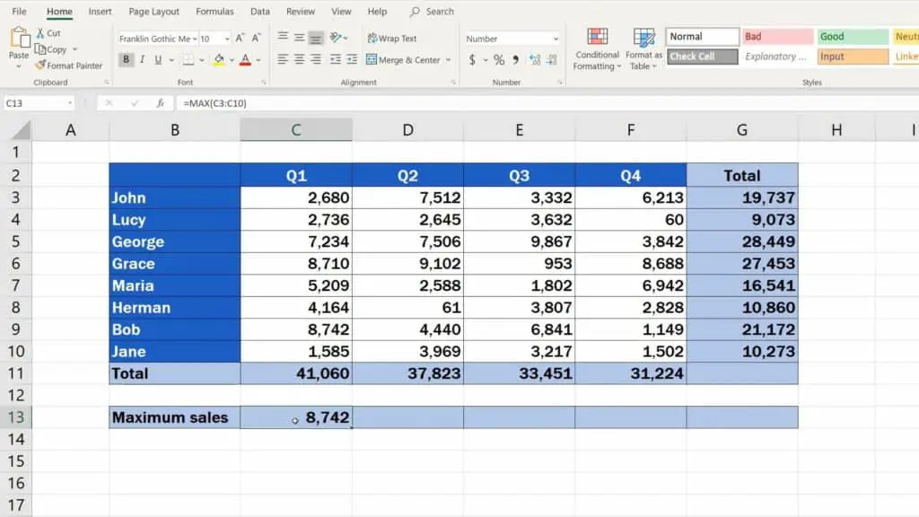
If you need to look for the largest number in any of the data tables you created, you can follow these steps.
And there’s more to that.
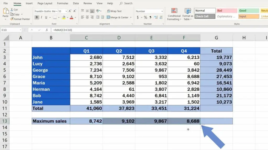
How to Find the Largest Number in All Quarters
To find out maximum sales in all quarters, just click on the cell containing the function and through its right bottom corner drag the formula through the rest of the cells.
Like this! Easy, right?
Are you interested in:
If you found this tutorial helpful, give us a ‘like’ and watch other video tutorials by EasyClick Academy. Learn how to use Excel in a quick and easy way!
Is this your first time on EasyClick? We’ll be more than happy to welcome you in our online community. Hit that Subscribe button on our YouTube channel and join the EasyClickers!
Источник
MAX function in Excel: formula examples to find and highlight highest value
 by Svetlana Cheusheva, updated on March 14, 2023
The tutorial explains the MAX function with many formula examples that show how to find highest value in Excel and highlight largest number in your worksheet.
MAX is one of the most straightforward and easy-to-use Excel functions. However, it does have a couple of tricks knowing which will give you a big advantage. Say, how do you use the MAX function with conditions? Or how would you extract the absolute largest value? This tutorial provides more than one solution for these and other related tasks.
Excel MAX function
The MAX function in Excel returns the highest value in a set of data that you specify.
The syntax is as follows:
Where number can be represented by a numeric value, array, named range, a reference to a cell or range containing numbers.
Number1 is required, number2 and subsequent arguments are optional.
The MAX function is available in all versions of Excel for Office 365, Excel 2019, Excel 2016, Excel 2013, Excel 2010, Excel 2007, and lower.
How to make a MAX formula in Excel
To create a MAX formula in its simplest from, you can type numbers directly in the list of arguments, like this:
In practice, it’s quite a rare case when numbers are «hardcoded». For the most part, you will deal with ranges and cells.
The fastest way to build a Max formula that finds the highest value in a range is this:
- In a cell, type =MAX(
- Select a range of numbers using the mouse.
- Type the closing parenthesis.
- Press the Enter key to complete your formula.
For example, to work out the largest value in the range A1:A6, the formula would go as follows:
=MAX(A1:A6) 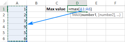
If your numbers are in a contiguous row or column (like in this example), you can get Excel to make a Max formula for you automatically. Here’s how:
- Select the cells with your numbers.
- On the Home tab, in the Formats group, click AutoSum and pick Max from the drop-down list. (Or click AutoSum >Max on the Formulas tab in the Function Library group.)
This will insert a ready-to-use formula in a cell below the selected range, so please make sure there is at least one blank cell underneath the list of numbers that you’ve selected: 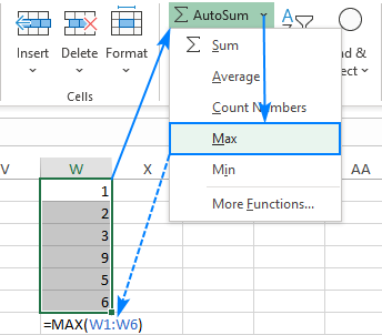
5 things to know about MAX function
To successfully use Max formulas your worksheets, please remember these simple facts:
- In the current versions of Excel, a MAX formula can accept up to 255 arguments.
- If the arguments do not contain a single number, the MAX function returns zero.
- If the arguments contain one or more error values, an error is returned.
- Empty cells are ignored.
- Logical values and text representations of numbers supplied directly in the list of arguments are processed (TRUE evaluates as 1, FALSE evaluates as 0). In references, logical and text values are ignored.
How to use MAX function in Excel – formula examples
Below you will find a few typical uses of the Excel MAX function. In many cases, there are a few different solutions for the same task, so I encourage you to test all the formulas to choose the one best suited for your data type.
How to find max value in a group
To extract the largest number in a group of numbers, supply that group to the MAX function as a range reference. A range can contain as many rows and columns as you desire. For example, to get the highest value in the range C2:E7, use this simple formula:
=MAX(C2:E7) 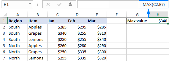
Find highest value in non-adjacent cells or ranges
To make a MAX formula for non-contiguous cells and ranges, you need to include a reference to each individual cell and/or range. The following steps will help you to do that quickly and flawlessly:
- Start typing a Max formula in a cell.
- After you’ve typed the opening parenthesis, hold down the Ctrl key and select the cells and ranges in the sheet.
- After selecting the last item, release Ctrl and type the closing parenthesis.
- Press Enter.
Excel will use an appropriate syntax automatically, and you will get a formula similar to this:
As shown in the screenshot below, the formula returns the maximum sub-total value from rows 5 and 9: 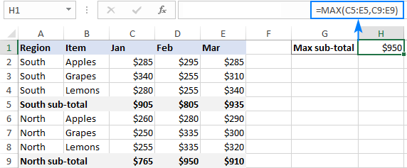
How to get max (latest) date in Excel
In the internal Excel system, dates are nothing else but serial numbers, so the MAX function handles them without a hitch.
For instance, to find the latest delivery date in C2:C7, make a usual Max formula that you’d use for numbers:
=MAX(C2:C7) 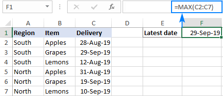
MAX function in Excel with conditions
When you wish to get the maximum value based on conditions, there are several formulas for you to choose from. To make sure that all the formulas return the identical result, we will test them on the same set of data.
The task: With the items listed in B2:B15 and sales figures in C2:C15, we aim to find the highest sale for a specific item input in F1 (please see the screenshot at the end of this section).
Excel MAX IF formula
If you a looking for a formula that works in all versions of Excel 2000 through Excel 2019, use the IF function to test the condition, and then pass the resulting array to the MAX function:
For the formula to work, it must press Ctrl + Shift + Enter simultaneously to enter it as an array formula. If all done correctly, Excel will enclose your formula in , which is a visual indication of an array formula.
It is also possible to evaluate several conditions in a single formula, and the following tutorial shows how: MAX IF with multiple conditions.
Non-array MAX IF formula
If you don’t like using array formulas in your worksheets, then combine MAX with the SUMPRODUCT function that processes arrays natively:
For more information, please see MAX IF without array.
MAXIFS function
In Excel 2019 and Excel for Office 365, there is a special function named MAXIFS, which is designed to find the highest value with up to 126 criteria.
In our case, there is just one condition, so the formula is as simple as:
=MAXIFS(C2:C15, B2:B15, F1)
For the detailed explanation of the syntax, please see Excel MAXIFS with formula examples.
The below screenshot shows all 3 formulas in action: 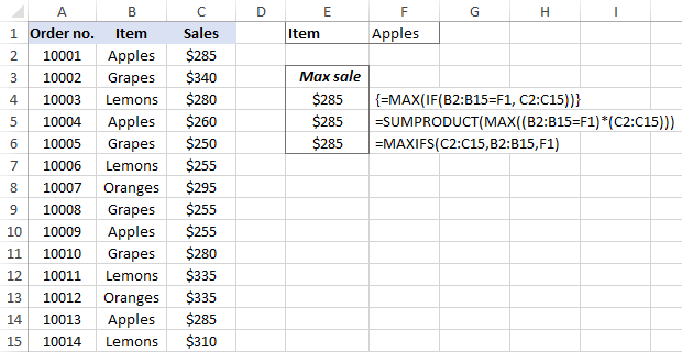
Get max value ignoring zeros
This is, in fact, a variation of conditional MAX discussed in the previous example. To exclude zeros, use the «not equal to» logical operator and put the expression «<>0″ in either the criteria of MAXIFS or the logical test of MAX IF.
As you understand, testing this condition only makes sense in case of negative numbers. With positive numbers, this check is superfluous because any positive number is greater than zero.
To give it a try, let’s find the lowest discount in the range C2:C7. As all the discounts are represented by negative numbers, the smallest discount is actually the largest value.
MAX IF
Be sure to press Ctrl + Shift + Enter to correctly complete this array formula:
MAXIFS
It’s a regular formula, and a usual Enter keystroke will suffice.
=MAXIFS(C2:C7,C2:C7,»<>0″) 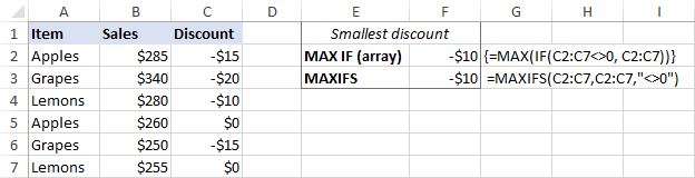
Find highest value ignoring errors
When you work with a large amount of data driven by various formulas, chances are that some of your formulas will result in errors, which will cause a MAX formula to return an error too.
As a workaround, you can use MAX IF together with ISERROR. Given that you are searching in the range A1:B5, the formula takes this shape:
To simplify the formula, use the IFERROR function instead of the IF ISERROR combination. This will also make the logic a bit more obvious – if there’s an error in A1:B5, replace it with an empty string (»), and then get the maximum value in the range:
A fly in the ointment is that you need to remember to press Ctrl + Shift + Enter because this only works as an array formula.
In Excel 2019 and Excel for Office 356, the MAXIFS function can be a solution, provided that your data set contains at least one positive number or zero value:
Since the formula searches for the highest value with the condition «greater than or equal to 0», it won’t work for a data set consisting of solely negative numbers.
All these limitations are not good, and we are evidently in need of a better solution. The AGGREGATE function, which can perform a number of operations and ignore error values, fits perfectly:
=AGGREGATE(4, 6, A1:B5)
The number 4 in the 1st argument indicates the MAX function, the number 6 in the 2nd argument is the «ignore errors» option, and A1:B5 is your target range.
Under perfect circumstances, all three formulas will return the same result: 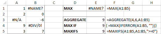
How to find absolute max value in Excel
When working with a range of positive and negative numbers, sometimes you may wish to find the largest absolute value regardless of the sign.
The first idea that comes to mind is to get the absolutes values of all numbers in the range by using the ABS function and feed those to MAX:
This is an array formula, so don’t forget to confirm it with the Ctrl + Shift + Enter shortcut. Another caveat is that it only works with numbers and results in an error in case of non-numeric data.
Not happy with this formula? Then let us build something more viable 🙂
What if we find the minimum value, reverse or ignore its sign, and then evaluate along with all other numbers? Yep, that will work perfectly as a normal formula. As an extra bonus, it handles text entries and errors just fine:
With the source numbers in A1:B5, the formulas go as follows.
Array formula (completed with Ctrl + Shift + Enter):
Regular formula (completed with Enter):
The below screenshot shows the results: 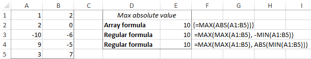
Return the maximum absolute value preserving the sign
In some situations, you may have a need to find the largest absolute value but return the number with its original sign, not the absolute value.
Assuming the numbers are in cells A1:B5, here’s the formula to use:
=IF(ABS(MAX(A1:B5))>ABS(MIN(A1:B5)), MAX(A1:B5), MIN(A1:B5))
Complex at first sight, the logic is quite easy to follow. First, you find the largest and smallest numbers in the range and compare their absolute values. If the absolute max value is greater than the absolute min value, the maximum number is returned, otherwise – the minimum number. Because the formula returns the original and not absolute value, it keeps the sign information: 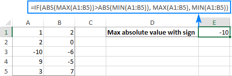
How to highlight max value in Excel
In situation when you want to identify the largest number in the original data set, the fastest way is to highlight it with Excel conditional formatting. The below examples will walk you through two different scenarios.
Highlight highest number in a range
Microsoft Excel has a predefined rule to format top ranked values, which suits our needs perfectly. Here are the steps to apply it:
- Select your range of numbers (C2:C7 in our case).
- On the Home tab, in the Styles group, click Conditional formatting > New Rule.
- In the New Formatting Rule dialog box, choose Format only top or bottom ranked values.
- In the lower pane, pick Top from the drop-down list and type 1 in the box next to it (meaning you want to highlight just one cell containing the largest value).
- Click the Format button and select the desired format.
- Click OK twice to close both windows.
Done! The highest value in the selected range is automatically highlighted. If there is more than one max value (duplicates), Excel will highlight them all: 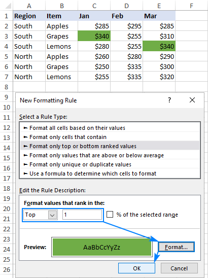
Highlight max value in each row
Since there is no built-in rule to make the highest value stand out from each row, you will have to configure your own one based on a MAX formula. Here’s how:
- Select all the rows in which you want to highlight max values (C2:C7 in this example).
- On the Home tab, in the Styles group, click New Rule >Use a formula to determine which cells to format.
- In the Format values where this formula is true box, enter this formula:
Where C2 is the leftmost cell and $C2:$E2 is the first row range. For the rule to work, be sure to lock the column coordinates in the range with the $ sign.
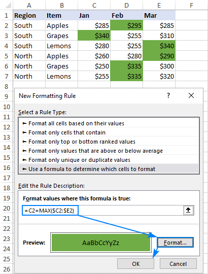
Tip. In a similar manner, you can highlight the highest value in each column. The steps are exactly the same, except that you write a formula for the first column range and lock the row coordinates: =C2=MAX(C$2:C$7)
Excel MAX function not working
MAX is one of the most straightforward Excel functions to use. If against all expectations it does not work right, it’s most likely to be one of the following issues.
MAX formula returns zero
If a normal MAX formula returns 0 even though there are higher numbers in the specified range, chances are those numbers are formatted as text. It’s especially the case when you run the MAX function on data driven by other formulas. You can check this by using the ISNUMBER function, for example:
If the above formula returns FALSE, the value in A1 is not numeric. Meaning, you should troubleshoot the original data, not a MAX formula.
MAX formula returns #N/A, #VALUE or other error
Please check the referenced cells carefully. If any of the referenced cells contains an error, a MAX formula will result in the same error. To bypass this, see how to get the max value ignoring all errors.
That’s how to find max value in Excel. I thank you for reading and hope to see you on our blog soon!
Источник

Finding the biggest number within a range of Excel cells is super easy.
Same for picking the smallest number.
There are many situations where you need to find the biggest/smallest, highest/lowest, longest/shortest value in a set of data. For example,
- Which employee has taken the most sick days this year?
- What has been the largest expense this year?
- What is the lowest cost per lead from our advertising campaigns?
Clickable Table of Contents
1. How to find the biggest number in Excel
Use the MAX function to find the biggest number in a list (or tallest, longest, most etc.)
=MAX(number1, number 2 …)
For example:
=MAX(A1,A2,A3)
=MAX(A1:A10)
=MAX(TestScores)
2. How to find the smallest number in Excel
Use the MIN function to find the smallest number in a list (or shortest, lowest, least etc.)
=MIN(number1, number 2 …)
For example:
=MIN(B1,B2,B3)
=MIN(B1:B10)
=MIN(DepartmentSpend)
The MAX and MIN functions can be selected from the AutoSum drop down menu, or by typing it directly into the cell.
Let’s say you have values in cells A1 to A10,
To use the AutoSum tool:
1. Select the 10 cells.
2. Click the drop-down arrow on the AutoSum icon.
3. Choose MAX or MIN.
Or if you want to write the formula manually:
1. Select a blank cell that will contain the extracted value.
2. Type ‘=MAX(’ or ‘=MIN(’.
3. With your mouse, select the range of cells that contains your data.
4. Type the closing bracket.
5. Press Enter.
Using either technique, the final formula will look like:
=MAX(A1:A10)
3. What next?
I hope you found plenty of value in this post. I’d love to hear your biggest takeaway in the comments below together with any questions you may have.
Have a fantastic day.


About the author
Jason Morrell
Jason loves to simplify the hard stuff, cut the fluff and share what actually works. Things that make a difference. Things that slash hours from your daily work tasks. He runs a software training business in Queensland, Australia, lives on the Gold Coast with his wife and 4 kids and often talks about himself in the third person!
SHARE