
Excel for Microsoft 365 Excel for Microsoft 365 for Mac Excel for the web Excel 2021 Excel 2021 for Mac Excel 2019 Excel 2019 for Mac Excel 2016 Excel 2016 for Mac Excel 2013 Excel 2010 Excel 2007 Excel for Mac 2011 Excel Starter 2010 More…Less
This article describes the formula syntax and usage of the IRR function in Microsoft Excel.
Description
Returns the internal rate of return for a series of cash flows represented by the numbers in values. These cash flows do not have to be even, as they would be for an annuity. However, the cash flows must occur at regular intervals, such as monthly or annually. The internal rate of return is the interest rate received for an investment consisting of payments (negative values) and income (positive values) that occur at regular periods.
Syntax
IRR(values, [guess])
The IRR function syntax has the following arguments:
-
Values Required. An array or a reference to cells that contain numbers for which you want to calculate the internal rate of return.
-
Values must contain at least one positive value and one negative value to calculate the internal rate of return.
-
IRR uses the order of values to interpret the order of cash flows. Be sure to enter your payment and income values in the sequence you want.
-
If an array or reference argument contains text, logical values, or empty cells, those values are ignored.
-
-
Guess Optional. A number that you guess is close to the result of IRR.
-
Microsoft Excel uses an iterative technique for calculating IRR. Starting with guess, IRR cycles through the calculation until the result is accurate within 0.00001 percent. If IRR can’t find a result that works after 20 tries, the #NUM! error value is returned.
-
In most cases you do not need to provide guess for the IRR calculation. If guess is omitted, it is assumed to be 0.1 (10 percent).
-
If IRR gives the #NUM! error value, or if the result is not close to what you expected, try again with a different value for guess.
-
Remarks
IRR is closely related to NPV, the net present value function. The rate of return calculated by IRR is the interest rate corresponding to a 0 (zero) net present value. The following formula demonstrates how NPV and IRR are related:
NPV(IRR(A2:A7),A2:A7) equals 1.79E-09 [Within the accuracy of the IRR calculation, the value is effectively 0 (zero).]
Example
Copy the example data in the following table, and paste it in cell A1 of a new Excel worksheet. For formulas to show results, select them, press F2, and then press Enter. If you need to, you can adjust the column widths to see all the data.
|
Data |
Description |
|
|
-$70,000 |
Initial cost of a business |
|
|
$12,000 |
Net income for the first year |
|
|
$15,000 |
Net income for the second year |
|
|
$18,000 |
Net income for the third year |
|
|
$21,000 |
Net income for the fourth year |
|
|
$26,000 |
Net income for the fifth year |
|
|
Formula |
Description |
Result |
|
=IRR(A2:A6) |
Investment’s internal rate of return after four years |
-2.1% |
|
=IRR(A2:A7) |
Internal rate of return after five years |
8.7% |
|
=IRR(A2:A4,-10%) |
To calculate the internal rate of return after two years, you need to include a guess (in this example, -10%). |
-44.4% |
Need more help?
Want more options?
Explore subscription benefits, browse training courses, learn how to secure your device, and more.
Communities help you ask and answer questions, give feedback, and hear from experts with rich knowledge.
IRR (Internal Rate of Return) is an indicator of the internal rate of return of an investment project. It is often used to compare different proposals for the growth and profitability perspective. The higher the IRR, the greater is the growth prospects for this project. Let’s calculate the interest rate of IRR in Excel.
The economic meaning of the indicator
Other names: the internal rate of profitability (profit, discount), the internal factor of recoupment (efficiency), an internal norm.
The IRR coefficient shows the minimum level of profitability of the investment project. In another way: it is the interest rate at which the net present value is zero.
The formula for calculating the indicator manually:
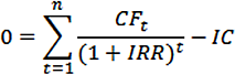
- CFt – is cash flow for a certain period of time t;
- IC – is investments in the project at the stage of entry (launch);
- t – is the time period.
In practice, the IRR ratio is often compared with the weighted average capital cost (WACC):
- IRR above WACC: this project should be carefully considered.
- IRR below WACC: it is inappropriate to invest in the development of the project.
- Indicators are equal: the minimum permissible level (the enterprise needs to adjust the cash flow).
Often the IRR is compared in percentages on a bank deposit. If the interest on the deposit is higher, then it is better to look for another investment project.
Example of calculating IRR in Excel
You can quickly calculate the IRR using the built-in Excel IRR function. Syntax:
- Range of values — reference to cells with numerical arguments for which you want to calculate the internal rate of return (at least one cash flow must have a negative value).
- Assumption — a value that is supposedly close to the value of the IRR (the argument is optional; but if the function produces an error, the argument must be specified).
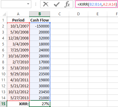
Take the conventional figures:
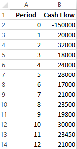
The initial costs were 150,000, so this numerical value entered the table with a minus sign. Now we’ll find the IRR. The formula for calculation in Excel:
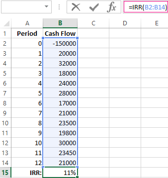
Calculations showed that the internal rate of return on the investment project is 11%. For further analysis, the value is compared with the interest rate of the bank deposit, or the cost of the capital of the project, or IRR of another investment project.
We calculated the IRR for regular cash income. The IRR function cannot be used with non-systematic income because the discount rate for each cash flow will vary. We solve the problem with the help of the function XIRR.
We modify the table with the initial data for the example:
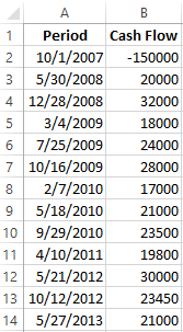
The mandatory arguments of the XIRR function are next:
- Values are cash flows;
- Dates are an array of dates in the appropriate format.
The formula for calculating IRR for non-systematic payments:
A significant drawback of the two previous functions is the unrealistic assumption about the rate of reinvestment. It is recommended to use the MIRR function to correctly consider the assumption of reinvestment.
Arguments:
- Values are payments;
- Financing rate is interest paid for funds in circulation;
- The rate of reinvestment.
Suppose that the discount is 10%. There is a possibility of reinvesting the revenues at a rate of 7% per annum. We calculate the modified internal rate of return:
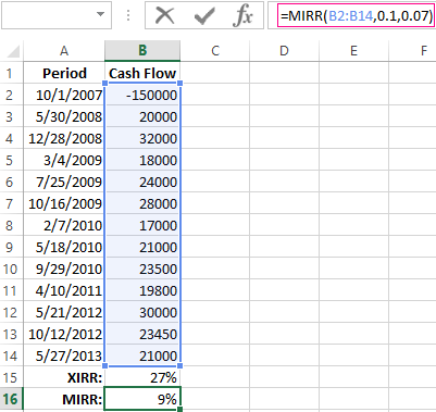
The resulting rate of return is three times less than the previous result. And it’s below the financing. Therefore, the profitability of this project is doubtful.
Graphical method for calculating IRR in Excel
The IRR value can be found graphically by plotting the net present value (NPV) versus the discount rate. NPV is one of the methods for evaluating an investment project which is based on the methodology of discounting cash flows.
For example, take a project with the following structure of cash flows:
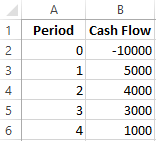
You can use the NPV function to calculate NPV in Excel:
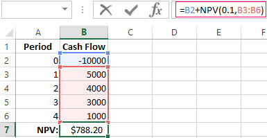
Since the first cash flow occurred in the zero periods, it does not have to enter the value array. The initial investment should be added to the value calculated by the NPV function.
The function discounted cash flows for periods from 1 to 4 at a rate of 10% (0.10). It is impossible to accurately determine the discount rate and all cash flows when analyzing a new investment project. It makes sense to look at the dependence of NPV on these indicators. In particular, look how it depends on the cost of capital (discount rates).
We calculate NPV for different discount rates:
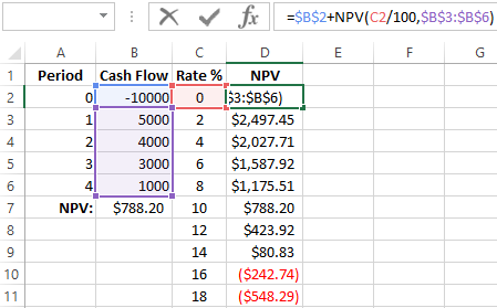
Let’s see the results on the chart:
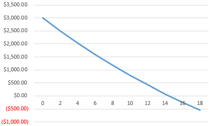
Remember that the IRR is the discount rate at which the NPV of the analyzed project is zero. Therefore, the intersection point of the NPV graph with the abscissa axis is the internal profitability of the enterprise.
What Is the Internal Rate of Return (IRR)?
The internal rate of return (IRR) is the discount rate providing a net value of zero for a future series of cash flows. Both the IRR and net present value (NPV) are used when selecting investments based on their returns.
Excel has three functions for calculating the internal rate of return that include Internal Rate of Return (IRR), Modified Internal Rate of Return (MIRR), and Internal Rate of Return with time periods (XIRR).
The IRR function calculates the internal rate of return for a series of cash flows, the MIRR function works with interest rates for borrowing and investing, and the XIRR function calculates a more accurate internal rate of return as it considers time periods.
Key Takeaways
• The internal rate of return (IRR) is the discount rate providing a net value of zero for a future series of cash flows.
• Excel has three functions for calculating the internal rate of return.
• When using different borrowing rates of reinvestment, a modified internal rate of return (MIRR) applies.
• The XIRR function accounts for different time periods.
How to Calculate IRR in Excel
What Is Net Present Value?
NPV is the difference between the present value of cash inflows and the present value of cash outflows over time.
The net present value of a project depends on the discount rate used. So when comparing two investment opportunities, the choice of the discount rate, which is often based on a degree of uncertainty, will have a considerable impact.
In the example below, using a 20% discount rate, investment #2 shows higher profitability than investment #1. When opting instead for a discount rate of 1%, investment #1 shows a return bigger than investment #2. Profitability often depends on the sequence and importance of the project’s cash flow and the discount rate applied to those cash flows.
How IRR and NPV Differ
The main difference between the IRR and NPV is that NPV is an actual amount while the IRR is the interest yield as a percentage expected from an investment.
Investors typically select projects with an IRR that is greater than the cost of capital. However, selecting projects based on maximizing the IRR as opposed to the NPV could result in suboptimal economic outcomes.
IRR represents the actual annual return on investment only when the project generates zero interim cash flows, or if those investments can be invested at the current IRR.
Calculating IRR in Excel
The IRR is the discount rate that can bring an investment’s NPV to zero. When the IRR has only one value, this criterion becomes more interesting when comparing the profitability of different investments.
In our example, the IRR of investment #1 is 48% and, for investment #2, the IRR is 80%. This means that in the case of investment #1, with an investment of $2,000 in 2013, the investment will yield an annual return of 48%. In the case of investment #2, with an investment of $1,000 in 2013, the yield will bring an annual return of 80%.
If no parameters are entered, Excel starts testing IRR values differently for the entered series of cash flows and stops as soon as a rate is selected that brings the NPV to zero. If Excel does not find any rate reducing the NPV to zero, it shows the error «#NUM.»
If the second parameter is not used and the investment has multiple IRR values, we will not notice because Excel will only display the first rate it finds that brings the NPV to zero.
In the image below, for investment #1, Excel does not find the NPV rate reduced to zero, so we have no IRR.
The image below also shows investment #2. If the second parameter is not used in the function, Excel will find an IRR of -10%. On the other hand, if the second parameter is used (i.e., = IRR ($ C $ 6: $ F $ 6, C12)), there are two IRRs rendered for this investment, which are -10% and 216%.
If the cash flow sequence has only a single cash component with one sign change (from + to — or — to +), the investment will have a unique IRR. However, most investments begin with a negative flow and a series of positive flows as the first investments come in. Profits then, hopefully, subside, as was the case in our first example.
In the image below, we calculate the IRR. To do this, we simply use the Excel IRR function:
Calculating MIRR in Excel
When a company uses different borrowing rates of reinvestment, the modified internal rate of return (MIRR) applies.
In the image below, we calculate the IRR of the investment as in the previous example but taking into account that the company will borrow money to plow back into the investment (negative cash flows) at a rate different from the rate at which it will reinvest the money earned (positive cash flow). The range C5 to E5 represents the investment’s cash flow range, and cells D10 and D11 represent the rate on corporate bonds and the rate on investments.
The image below shows the formula behind the Excel MIRR. We calculate the MIRR found in the previous example with the MIRR as its actual definition. This yields the same result: 56.98%.
(
−
NPV
(
rrate, values
[
positive
]
)
×
(
1
+
rrate
)
n
NPV
(
frate, values
[
negative
]
)
×
(
1
+
frate
)
)
1
n
−
1
−
1
begin{aligned}left(frac{-text{NPV}(textit{rrate, values}[textit{positive}])times(1+textit{rrate})^n}{text{NPV}(textit{frate, values}[textit{negative}])times(1+textit{frate})}right)^{frac{1}{n-1}}-1end{aligned}
(NPV(frate, values[negative])×(1+frate)−NPV(rrate, values[positive])×(1+rrate)n)n−11−1
Calculating XIRR in Excel
The XIRR function takes into consideration different periods. To use this function, Excel requires both the cash flow amounts as well as the dates on which those cash flows are paid.
In the example below, the cash flows are not disbursed at the same time each year – as is the case in the above examples. Rather, they are happening at different periods. We use the XIRR function below to solve this calculation. We first select the cash flow range (C5 to E5) and then select the range of dates on which the cash flows are realized (C32 to E32).
For investments with cash flows received or cashed at different moments in time for a firm that has different borrowing rates and reinvestments, Excel does not provide functions that can be applied to these situations although they are probably more likely to occur.
The internal rate of return (IRR) is a concept in financial modeling commonly used in combination with net present value (NPV). The formula in Excel is used to estimate the rate of return an investment would give based on a series of cash flows, usually presented as a percentage (‘3%’). The NPV, on the other hand, is expressed as a cardinal number (‘3’). Both play a key role in making investment decisions when presented with more than one opportunity, as we will show here.
This article will provide step-by-step guidance on how to use the IRR formula to effectively calculate the IRR for investment decisions.
How to use the IRR function in Excel?
We will first explain how to use the IRR function in Excel to calculate the rate of annual return for an initial investment. If you need to calculate return rates for different times periods or a future value, Excel also offers a variety of financial functions, i.e. XIRR, or MIRR.
What is the formula for calculating IRR?
The syntax for the IRR formula is:
=IRR(values,[guess])
- values: This argument is required. It refers to the cash flows, the initial investment (as a negative figure), and net income (as a positive figure).
IMPORTANT: It is important that the initial investment and cash flows maintain the same sequence in the IRR formula will interpret in this very order. Moreover, for the IRR function to work properly, the argument should be a number. If it is a logical value, text, or an empty cell, it will be ignored.
- [guess]: This argument is optional. It is an estimation of the number closest to the expected IRR (as there can be two). If not included, the argument will show the default value of 0.1 (=10%).
Let’s now apply the IRR formula, to the following scenario:
You are a business owner and you are presented with two investment opportunities, A and B. The first has an initial investment of $2,500,000.00, whereas the second has one of €2,800,000.00. The net income for each is presented on a yearly basis. The IRR function can help you get an idea of what the return rate would be based on the initial investment and the yearly cash inflows:
- 1. Option A has an initial investment of $2,500,000.00 with the following yearly cash flows.

- 2. Type in ‘IRR’ in the cell you wish to showcase the IRR value.

- 3. As soon as you select from the drop-down menu, you will automatically be prompted to select the cell range that you wish to perform the IRR calculation on.
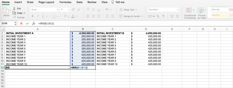
- 4. Once you press the Return key you will be shown the IRR percentage. Remember that IRR is represented as a percentage, whereas NPV is a cardinal number. Here, we get a return of 5%.

- 5. Now, let’s calculate the IRR for Option B with an initial investment of $2,800,000.00 and the following yearly cash flows.

- 6. We would input the formula in the same way we did previously in steps 2-3.

- 7. Here, we get an IRR of 8%.

The information obtained so far would help us decide solely based on the IRR; it is common practice to go for the higher percentage. Considering that Option A provides an IRR of 5% and B of 8%, we would opt for investing in project B. However, if the cash flows were on a monthly basis, our decision-making could be more precise. By following these steps, you can easily learn how to calculate IRR in Excel for monthly cash flow.
How to calculate IRR using NPV in Excel?
As mentioned in the Introduction, the NPV is expressed as a cardinal number, as opposed to the IRR which is expressed as a percentage. It is used to calculate the difference between current cash inflow and outflow over a period of time. Make note that the “rate” referred to in the NPV formula is not the same as the rate obtained using the IRR formula shown previously:
=NPV(rate, values)
- rate: refers to the discount rate for the investment period. This discount rate is a generic term used to refer to any rate that is established, subjectively or objectively, to discount future cash flows with. Moreover, for more reliable decision-making, we should always apply a lower and a higher discount rate for all investment options.
- values: refer to the initial investment (represented as a negative value) and the cash inflows over the given time periods.
Let’s say that we apply a 5% discount rate (this could represent the lower rate) to both investment opportunities.
- 1. Type in ‘NPV’ in the cell you want to obtain the NPV formula.

- 2. As the first parameter corresponds to the discount rate, we first need to add cell B13 followed by the sum of cash flows, and finally add all to the initial investment.

- 3. Press the Return key to obtain the NPV value ($50,196.47).

- 4. To calculate the NPV for investment option B, follow steps 1-3.

As mentioned before, we would now need to calculate the NPV for a higher discount rate (8%) for both investment opportunities. Once again, let’s start with option A.
- 5. We have included a second row where we will calculate the NPV applied to the same values as before, but this time include cell B15 as the discount rate.

- 6. Proceed to apply values to the NPV formula and press the “return” key to obtain the result:

- 7. For investment option B, we have followed steps 6 and 7 and obtained the following:

Based on the obtained results, we decide on Option B. Why? Because both the NPV and IRR are higher in both discount rate scenarios:

The IRR formula can only be used in instances where the cash flow distribution occurs over the same time periods (yearly, monthly, etc.). If you want to calculate the rate of return for different time periods, use the XIRR formula in Excel. This selects the cash flow range and then the range of dates on which the cash flows are made.
How to Use GOOGLEFINANCE Function in Google Sheets?
Import current or historical financial market data from Google Finance & monitor real-time. Here’s how to use the GOOGLEFINANCE function in Google Sheets
READ MORE

How do you calculate IRR manually?
If you are advanced in math or aren’t interested in calculating IRR in Excel, this is what you would need to do to calculate IRR manually:
- 1. Estimate two discount rate values (i.e., 4% and 8%) to try and set the NPV to zero.
- 2. Calculate the NPVs using 4% and 8% and try to get as close to zero as you can.
- 3. Once you determine your two discount rate values and the two NPVs, you can use this formula to calculate the IRR:
IRR = R1 + ( (NPV1 * (R2 - R1)) / (NPV1 - NPV2) )
- 4. R1 corresponds to the lower discount rate (4%) and R2 is the higher one (8%). NPV1, on the other hand, represents the higher NPV, and NPV2 the lower.
Want to Boost Your Team’s Productivity and Efficiency?
Transform the way your team collaborates with Confluence, a remote-friendly workspace designed to bring knowledge and collaboration together. Say goodbye to scattered information and disjointed communication, and embrace a platform that empowers your team to accomplish more, together.
Key Features and Benefits:
- Centralized Knowledge: Access your team’s collective wisdom with ease.
- Collaborative Workspace: Foster engagement with flexible project tools.
- Seamless Communication: Connect your entire organization effortlessly.
- Preserve Ideas: Capture insights without losing them in chats or notifications.
- Comprehensive Platform: Manage all content in one organized location.
- Open Teamwork: Empower employees to contribute, share, and grow.
- Superior Integrations: Sync with tools like Slack, Jira, Trello, and more.
Limited-Time Offer: Sign up for Confluence today and claim your forever-free plan, revolutionizing your team’s collaboration experience.
Conclusion
This article has explained the concepts of IRR and NPV, followed by a step-by-step process showing how to calculate IRR in Excel, how to use the IRR function in Excel in combination with NPV function, and finally broken down the use of IRR by explaining how to calculate IRR manually.
Whether you wish to explore further on financial functions or apply the functions seen in this post to real-time investments, you will find the article on How to use the GOOGLEFINANCE Function in Google Sheets very useful.
Hady is Content Lead at Layer.
Hady has a passion for tech, marketing, and spreadsheets. Besides his Computer Science degree, he has vast experience in developing, launching, and scaling content marketing processes at SaaS startups.
Originally published Jan 26 2022, Updated Mar 22 2023
When working with capital budgeting, IRR (Internal Rate of Return) is used to understand the overall rate of return a project would generate based on its future series of cash flows.
In this tutorial, I will show you how to calculate IRR in Excel, how is it different from another popular measure NPV, and different scenarios where you can use in-built IRR formulas in Excel.
Internal Rate of Return (IRR) Explained
IRR is a discount rate that is used to measure the return of an investment based on periodical incomes.
The IRR is shown as a percentage and can be used to decide whether the project (an investment) is profitable for a company or not.
Let me explain IRR with a simple example.
Suppose you’re planning to buy a company for $50,000 that will generate $10,000 every year for the next 10 years. You can use this data to calculate the IRR of this project, which is the rate of return you get on your investment of $50,000.
In the above example, the IRR comes out to be 15% (we will see how to calculate that later in the tutorial). This means that it is equivalent to you investing your money at a 15% rate or return for 10 years.
Once you have the IRR value, you can use it to make decisions. So if you have any other project where the IRR is more than 15%, you should invest in that project instead.
Or, if you’re planning to take a loan or raise capital and buy this project for $50,000, make sure that the cost of the capital is less than 15% (else you pay more as the cost of the capital than you make from the project).
IRR Function in Excel – Syntax
Excel allows you to calculate the internal rate of return using the IRR function. This function has the following parameters:
=IRR(values, [guess])
- values – an array of cells that contain numbers for which you want to calculate the internal rate of return.
- guess – a number that you guess is close to the result of the IRR (it’s not mandatory, and by default is 0.1 – 10%). This is used when there is a possibility of getting several results, and in that case, the function returns a result closest to a guess argument value.
Here are some important prerequisites for using the function:
- IRR function will only consider numbers in the specified range of cells. Any logical values or text strings in the array or reference argument would be ignored
- The amounts in the values parameter must be formatted as numbers
- The ‘guess’ parameter must be a percentage, formatted as decimal (if it’s provided)
- A cell where the function result is displayed must be formatted as a percentage
- The amounts occur at regular time intervals (months, quarters, years)
- One amount must be a negative cash flow (representing the initial investment), and other amounts should be positive cash flows, representing periodical incomes
- All amounts should be in chronological order because the function calculates the result based on the order of the amounts
In case you want to calculate the IRR value where the cash flow comes at different time intervals, you should use the XIRR function in Excel, which also allows you to specify the dates for each cash flow. An example of this is covered later in the tutorial
Now, let’s have a look at some example to better understand how to use the IRR function in Excel.
Calculating IRR For Varying Cash Flows
Suppose you have a dataset as shown below, where we have the initial investment of $30,000 and then varying cash flow/income from it for the next six years.

For this data, we need to calculate the IRR, which can be done using the below formula:
=IRR(D2:D8)

The result of the function is 8.22%, which is the IRR of the cash flow after six years.
Note: If the function returns a #NUM! error, you should fill the ‘guess’ parameter in the formula. This happens when the formula thinks that multiple values can be correct, and needs to have the guess value, in order to return the IRR nearest to the guess we provided. In most cases, you won’t need to use this though
Find Out When the Investment Yields Positive IRR
You can also calculate the IRR for every period in a cash flow and see when exactly the investment is starting to have a positive internal rate of return.
Suppose we have the below dataset where I have all the cashflows listed in column C.

The idea here is to find out the year in which the IRR of this investment turns positive (indicating when the project breaks even and becomes profitable).
To do this, instead of calculating the IRR for the entire project, we will find out the IRR for each year.
This can be done by using the below formula in cell D3 and then copying it for all the cells in the column.
=IRR($C$2:C3)

As you can see, the IRR after year 1 (values D2:D3) is -80%, after year 2 (D2:D4) -52%, etc.
This overview shows us that the investment of $30.000 with given cash flow has a positive IRR after the fifth year.
This can be useful when you’ve to choose from two project that have a similar IRR. It would be more lucrative to choose a project where the IRR turns positive faster, as it means less risk of recovering your initial capital.
Note that in the above formula, the reference of the range is mixed, that is the first cell reference ($C$2) is locked by having dollars signs before the row number and the column letter, and the second reference (C3) is not locked.
This makes sure that when you copy the formula down, it always considers the entire column till the row where the formula is applied.
Using IRR Function to Compare Multiple Projects
The IRR function in Excel can also be used to compare several projects’ investments and returns and see which project is the most profitable.
Suppose you have a dataset as shown below, where you have three projects with an initial investment (which is shown in negative as it’s an outflow) and then a series of positive cash flows.

To get the best project (that has the highest IRR, we will have to calculated the IRR for each project using the simple IRR formula:
=IRR(C2:C8)
The above formula will give the IRR for project 1. Similarly, you can also calculate the IRR for the other two projects.
As you can see:
- Project 1 has an IRR of 5.60%
- Project 2 has an IRR of 1.75%
- Project 3 has an IRR of 14.71%.

If we suppose that the cost of capital is 4.50%, we can conclude that investment 2 is not acceptable (as it will lead to a loss), while Investment 3 is the most profitable, with the highest internal rate of return.
So if you have to make a decision to invest in only one project, you should go with Project 3, and if you could invest in more than one projects, you can invest in Project 1 and 3.
Definition: If you’re wondering what’s cost of capital, it’s the money you will have to pay to get access to the money. For example, if you take $100K on loan at 4.5% per year, your cost of capital is 4.5%. Similarly, if you issue preferential shares promising a 5% return to get 100K, your cost of capital would be 5%. In real-life scenarios, a company usually raises money from various sources, and its cost of capital is a weighted average of all these capital sources.
Calculating IRR for Irregular Cashflows
One of the limitations of the IRR function in Excel is that the cashflows must be periodic with same interval between them.
But in real life, there can be instances, where your projects pay off in irregular intervals.
For example, below is a dataset where the cashflows take place at irregular intervals (see dates in column A).

In this example, we can not use the regular IRR function, but there is another function that can do this – the XIRR function.
XIRR function takes the cashflows as well as the dates, which allows it to account for irregular cashflows and give the correcyt IRR.
In this example, the IRR can be calculated using the below formula:
=XIRR(B2:B8,A2:A8)

In the above formula, the cashflows are specified as the first argument and the dates are specified as the second argument.
In case this formula returns a #NUM! error, you should enter the third argument with an approximate IRR that you expect. Don’t worry, it doesn’t have to be exact or even very close, just an approximation of what IRR you think it would yield. Doing this helps the formula iterate better and gives the result.
IRR vs NPV – Which is Better?
When it comes to evaluating projects, both NPV and IRR are used, but NPV is the more reliable method.
NPV is the Net Present Value method where you evaluate all the future cash flows and calculate what will be the net present value of all those cashflows.
If this value comes out to be higher than your initial outflow, then the project is profitable, else the project is not profitable.
On the other hand, when you calculate IRR for a project, it tells you what would be the rate of return all the future cash flow so that you get the amount equivalent to the current outflow. For example, if you’re spending $100K today on a project which has an IRR or 10%, it tells you that if you discount all the future cash flows at 10% discount rate, you will get $100K.
While both methods are used while evaluating projects, using the NPV method is more reliable. There is a possibility that you may get conflicting results when evaluating a project using the NPV and the IRR method.
In such a case, it is best to go with the recommendation you get using the NPV method.
In general, IRR method has some drawbacks, which make NPV method more reliable:
- Higher or method assumes that all the future cash flows generated from a project would be reinvested at the same rate of return (i.e., the IRR of the project). in most cases, this is an unreasonable assumption, as most of the cash flows would be reinvested into other projects which can have a different IR or insecurity such as bonds which would have a much lower rate of return.
- In case you have multiple outflows and inflows in the project, there would be multiple IRRs for that project. This again makes comparison a lot difficult.
Despite its shortcomings, IRR is a good way to evaluate a project and can be used in conjunction with the NPV method when you are deciding on which project(s) to choose.
In this tutorial, I showed you how to use the IRR function in Excel. I also covered how to calculate the IRR in case you have irregular cash flows using the XIRR function.
I hope you found this tutorial useful!
Other Excel tutorials you may also like:
- How to Calculate Average Annual Growth Rate (AAGR) in Excel
- How to Calculate Compound Interest in Excel + FREE Calculator
- How to Calculate Correlation Coefficient In Excel
- How to Calculate Standard Deviation In Excel
- Calculating Moving Average in Excel [Simple, Weighted, & Exponential]
- How to Calculate Compound Annual Growth Rate (CAGR) in Excel