
On the Insert tab, in the Text group, click Header & Footer. Excel displays the worksheet in Page Layout view. To add or edit a header or footer, click the left, center, or right header or footer text box at the top or the bottom of the worksheet page (under Header, or above Footer). Type the new header or footer text.
Contents
- 1 How do I make the first row a header in Excel?
- 2 How do I create a column header row in Excel?
- 3 How do I put a header and footer on every page in Excel?
- 4 Where is the header row in Excel?
- 5 What is a row header?
- 6 How do I show column and row headings in Excel?
- 7 What is header in Excel?
- 8 How do I copy a header to all sheets in Excel?
- 9 Why is my header not showing in Excel?
- 10 What are column headings?
- 11 What are row and column headers?
- 12 How do I show a chart title in Excel?
- 13 How do I format a text header in Excel?
- 14 How do you put a title on Excel?
- 15 How do I copy a header and footer to all pages?
- 16 How do I copy and paste a header?
- 17 Can you name rows in Excel?
- 18 How do I create a row label?
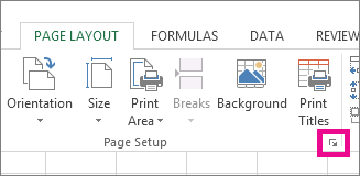
Click the [Page Layout] tab > In the “Page Setup” group, click [Print Titles]. Under the [Sheet] tab, in the “Rows to repeat at top” field, click the spreadsheet icon. Click and select the row you wish to appear at the top of every page. Press the [Enter] key, then click [OK].
How do I create a column header row in Excel?
Open the Spreadsheet
- Open the Spreadsheet.
- Open the spreadsheet where you want to have Excel make the top row a header row.
- Add a Header Row.
- Enter the column headings for your data across the top row of the spreadsheet, if necessary.
- Select the First Data Row.
How do I put a header and footer on every page in Excel?
If you want to add a header or footer to all sheets, select every sheet by right-clicking one of the sheet tabs at the bottom of the Excel screen and clicking “Select All Sheets” in the pop-up menu. It’s fairly common to put an Excel header on all pages of all worksheets in your document.
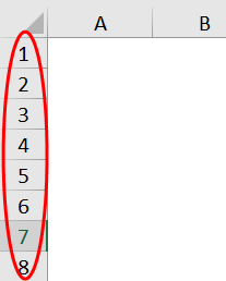
Microsoft Excel sheet has the capacity to hold a million rows with a numeric or text dataset in it. Row header or Row heading is the gray-colored column located on the left side of column 1 in the worksheet, which contains the numbers (1, 2, 3, etc.)
A row heading identifies a row on a worksheet. Row headings are at the left of each row and are indicated by numbers.
How do I show column and row headings in Excel?
On the Ribbon, click the Page Layout tab. In the Sheet Options group, under Headings, select the Print check box. , and then under Print, select the Row and column headings check box .
A header in excel: It is a section of the worksheet that appears at the top of each of the pages in the excel sheet or document. This remains constant across all the pages. It can contain information such as Page No., Date, Title or Chapter Name, etc.
Right-click on the sheet tab, Select Move or Copy, make sure that ‘Create a copy’ is checked. That copies the whole sheet including header/footer. Alternatively, select all the sheets by holding the Shift key down and clicking the first and last sheet tab. Then you can edit the header for all sheets at once.
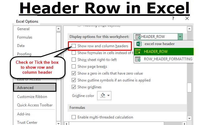
The Advanced options of the Excel Options dialog box. Make sure the Show Row and Column Headers check box is selected. If cleared, then the header area is not displayed. Click on OK.
What are column headings?
The column heading is a heading that identifies a column of a worksheet. Column headings are at the top of each column and are labeled A, B,… Z, AA, AB… . This example shows two columns, column A and column B.
What are row and column headers?
used to identify each column in the worksheet. The column header is located above row 1 in the worksheet. The row heading or row header is the gray-colored column located to the left of column 1 in the worksheet containing the numbers (1, 2, 3, etc.) used to identify each row in the worksheet.
How do I show a chart title in Excel?
Click the chart, and then click the Chart Design tab. Click Add Chart Element > Chart Title, and then click the title option that you want. Type the title in the Chart Title box. To format the title, select the text in the title box, and then on the Home tab, under Font, select the formatting that you want.
On the status bar, click the Page Layout View button. Select the header or footer text you want to change. On the Home tab in the Font group, set the formatting options that you want to apply to the header / footer.
How do you put a title on Excel?
Use a Header
- Click the “Insert” tab.
- Click the “Header & Footer” button on the ribbon.
- Click into the text box and type the spreadsheet title.
- Click into cell A1, the first cell on the spreadsheet.
- Type the title for the spreadsheet.
- Highlight the text you just typed.
How do I copy a header and footer to all pages?
Use the controls in the Navigation group to display the header or footer you want to copy. Select all the elements (text and graphics) in the header or footer. Press Ctrl+C. This copies the header or footer information to the Clipboard.
How do I copy and paste a header?
Double-click the header area to enable and open it. Click inside the header and highlight all of the section to copy. Right-click and select “Copy” or press “Ctrl-C” to copy the highlighted header.
Can you name rows in Excel?
Select the range you want to name, including the row or column labels. Select Formulas > Create from Selection. In the Create Names from Selection dialog box, designate the location that contains the labels by selecting the Top row,Left column, Bottom row, or Right column check box. Select OK.
How do I create a row label?
Row Labels
- Add a virtual column to the table.
- In the app formula field of the virtual column, enter a CONCATENATE expression that combines appropriate column values to form the row label.
- Reset the “Row Label” property for any existing row label column.
- Set the “Row Label” property of the virtual column.
Excel Header Row (Table of Contents)
- Header Row in Excel
- How to turn the Row Header on or off in Excel?
- Row Header formatting options in Excel
Microsoft Excel sheet has the capacity to hold a million rows with a numeric or text dataset in it.
Row header or Row heading is the gray-colored column located on the left side of column 1 in the worksheet, which contains the numbers (1, 2, 3, etc.) where it helps out to identify each row in the worksheet. Whereas the column header is the gray-colored row, it will usually be letters (A, B, C, etc.), which helps identify each column in the worksheet.
Row header label will help you out to identify & compare the information of the content when you are working with a huge number of data sets when it is difficult to accommodate the data in a single window or page & to compare information in your worksheet of excel.
Usually, a combination of column letters and row numbers helps out to create cell references. Row header will help you identify individual cells located at the intersection point between a column and row in a worksheet in excel.
Definition
Header rows are the label rows containing information that helps you identify the content of a particular column in a worksheet.
If the dataset table spans over several pages in an excel sheet print layout or towards the right if you scroll on & on, the header row will remain constant & stagnant, which usually repeat itself at the beginning of each new page.
How to turn the Header Row on or off in Excel?
Row headers in excel will always be visible all the time, even when you scroll the column data sets or values towards the right in the worksheet.
Sometimes, the row header in excel will not be displayed on a particular worksheet. It will be turned off in several cases, the main reason for turning them off is –
- Better or improved appearance of the worksheet in excel or
- To obtain or gain the extra screen space on worksheets containing a large number of tabular datasets.
- To take a screenshot or capture.
- When you take a printout of a tabular dataset, the row header or heading makes things complicated or confusing with the printed data set because of interference of row & column header; therefore, whenever you take a print out, the row header should always be turned off for each individual worksheet in the excel.
Now, let’s check out how to turn off the row headers or headings in Excel.
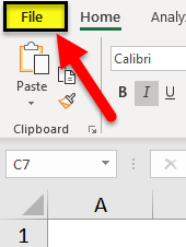
- Select or Click on the File option in the home toolbar of the menu to open the drop-down list.
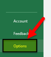
- Click on Options in the list present on the left-hand side to open the Excel Options dialog box.
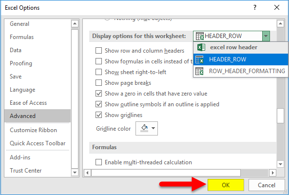
- Now, the Excel Options dialog box appears; in the left-hand panel of the excel options dialog box, select the Advanced option.
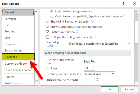
- Now, if you move the cursor down after the advanced option, you can observe Display options for this worksheet section located near the bottom of the right-hand pane of the dialog box; by default, it shows the row and column headers option always checked or ticked in.
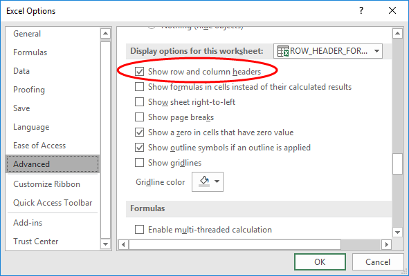
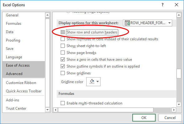
- If you want to turn off the row headers or headings in Excel, click on or uncheck the selection box of a checkbox in the Show row and column headers option.
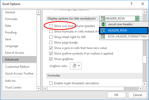
- Simultaneously, you can turn off the row and column headings for additional worksheets in the open workbook or current workbook of excel. It can be done by selecting the name of another worksheet under the drop-down box located next to the Display options.
- Once you have unchecked the box, Click OK to close the excel options dialog box, and you can return to the worksheet.
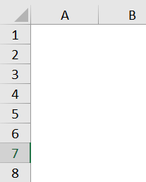
- Now, the above procedure disables the visibility of a row or column header.
When you try to open a new Excel file, the row header or heading is displayed by default of normal style or theme font similar to the workbook’s default format. This same normal style font is also applicable for all the worksheet in the workbook.
The default heading font is Calibri & the font size is 11. It can be changed based on your choice as per your requirement; whatever font style & size you apply will reflect in all the worksheets in a workbook of excel.
You have an option to format font & its size settings, with various options in format settings.
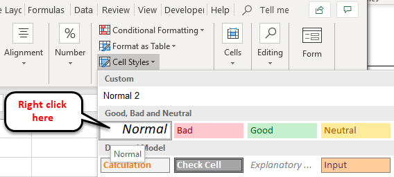
- In the Home tab of the Ribbon menu. Under the Styles group, select or click on Cell Styles to open the Cell Styles drop-down palette.
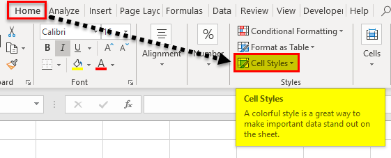
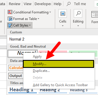
- In the dropdown, under Good, bad & neutral, Right-click or select on the box in the palette entitled Normal – it is also called a Normal style.
- Click on Modify option under normal.
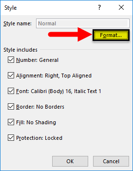
- A style dialog box appears; click on the Format in that window.
- Now, the Format Cells dialog box appears. In that, you can change the font size and its appearance, i.e. Font style or size.
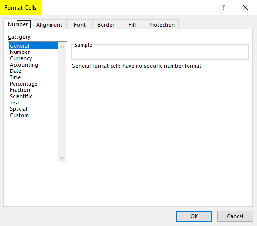
- I changed the font style & size, i.e. Calibri & font style to Regular, and I increased the font size to 16 from 11.
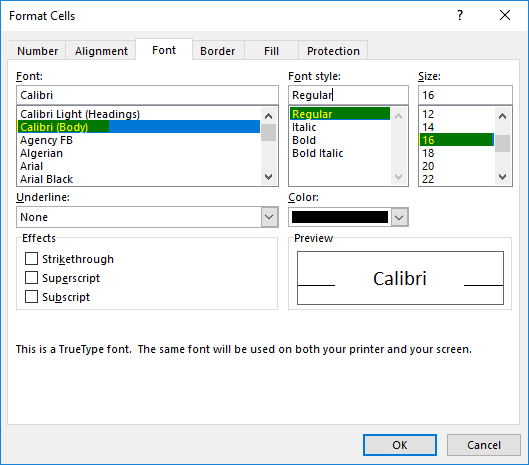
Once the desired changes are made, click OK twice, i.e. in the format cells dialog box & style dialog box based on your preference.
Note: Once you made changes in the font settings, you have to click on the save option in the workbook; otherwise, it will revert back to the default normal style or theme font (i.e.default heading font is Calibri & font size is 11).
Things to Remember
- Row header (with row number) make things easier to view or access the content when you try to navigate or scroll to another area or different parts of your worksheet at the same time in excel.
- An advantage of the header row is you can set this label row to print on all pages in excel or word; it is very significant & will be helpful for spreadsheets that span multiple pages.
Recommended Articles
This has been a guide to Header Row in Excel. Here we discuss how to turn row header on or off and row header formatting options in excel. You can also go through our other suggested articles –
- ROWS Function in Excel
- Column Header in Excel
- Excel Header and Footer
- Add Rows in Excel Shortcut
Содержание
- Overview of Excel tables
- Learn about the elements of an Excel table
- Create a table
- Working efficiently with your table data
- Export an Excel table to a SharePoint site
- Need more help?
- Headers and footers in a worksheet
- Add or change headers or footers in Page Layout view
- Need more help?
Overview of Excel tables
To make managing and analyzing a group of related data easier, you can turn a range of cells into an Excel table (previously known as an Excel list).

Note: Excel tables should not be confused with the data tables that are part of a suite of what-if analysis commands. For more information about data tables, see Calculate multiple results with a data table.
Learn about the elements of an Excel table
A table can include the following elements:
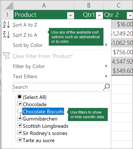
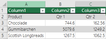
Header row By default, a table has a header row. Every table column has filtering enabled in the header row so that you can filter or sort your table data quickly. For more information, see Filter data or Sort data.
You can turn off the header row in a table. For more information, see Turn Excel table headers on or off.
Banded rows Alternate shading or banding in rows helps to better distinguish the data.
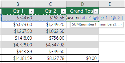
Calculated columns By entering a formula in one cell in a table column, you can create a calculated column in which that formula is instantly applied to all other cells in that table column. For more information, see Use calculated columns in an Excel table.
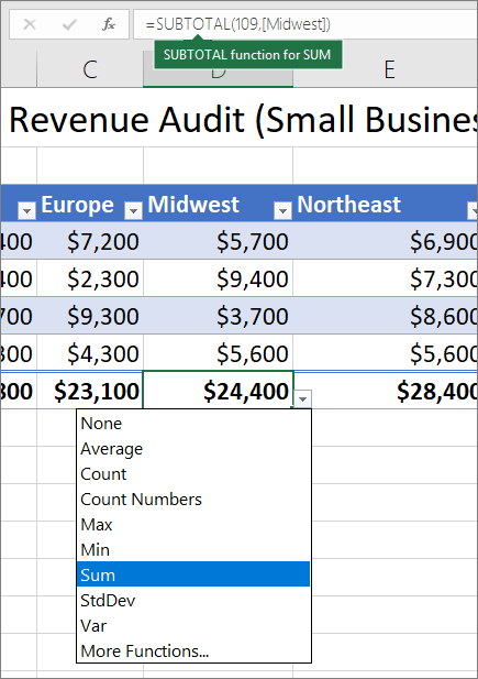
Total row Once you add a total row to a table, Excel gives you an AutoSum drop-down list to select from functions such as SUM, AVERAGE, and so on. When you select one of these options, the table will automatically convert them to a SUBTOTAL function, which will ignore rows that have been hidden with a filter by default. If you want to include hidden rows in your calculations, you can change the SUBTOTAL function arguments.
Sizing handle A sizing handle in the lower-right corner of the table allows you to drag the table to the size that you want.
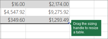
For other ways to resize a table, see Resize a table by adding rows and columns.
Create a table
You can create as many tables as you want in a spreadsheet.
To quickly create a table in Excel, do the following:
Select the cell or the range in the data.
Select Home > Format as Table.
Pick a table style.
In the Format as Table dialog box, select the checkbox next to My table as headers if you want the first row of the range to be the header row, and then click OK.
Working efficiently with your table data
Excel has some features that enable you to work efficiently with your table data:
Using structured references Instead of using cell references, such as A1 and R1C1, you can use structured references that reference table names in a formula. For more information, see Using structured references with Excel tables.
Ensuring data integrity You can use the built-in data validation feature in Excel. For example, you may choose to allow only numbers or dates in a column of a table. For more information on how to ensure data integrity, see Apply data validation to cells.
If you have authoring access to a SharePoint site, you can use it to export an Excel table to a SharePoint list. This way other people can view, edit, and update the table data in the SharePoint list. You can create a one-way connection to the SharePoint list so that you can refresh the table data on the worksheet to incorporate changes that are made to the data in the SharePoint list. For more information, see Export an Excel table to SharePoint.
Need more help?
You can always ask an expert in the Excel Tech Community or get support in the Answers community.
Источник
You can add headers or footers at the top or bottom of a printed worksheet in Excel. For example, you might create a footer that has page numbers, the date, and the name of your file. You can create your own, or use many built-in headers and footers.
Headers and footers are displayed only in Page Layout view, Print Preview, and on printed pages. You can also use the Page Setup dialog box if you want to insert headers or footers for more than one worksheet at a time. For other sheet types, such as chart sheets, or charts, you can insert headers and footers only by using the Page Setup dialog box.
Click the worksheet where you want to add or change headers or footers.
On the Insert tab, in the Text group, click Header & Footer.
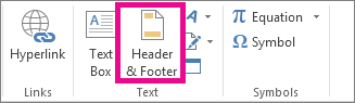
Excel displays the worksheet in Page Layout view.
To add or edit a header or footer, click the left, center, or right header or footer text box at the top or the bottom of the worksheet page (under Header, or above Footer).
Type the new header or footer text.
To start a new line in a header or footer text box, press Enter.
To include a single ampersand (&) in the text of a header or footer, use two ampersands. For example, to include «Subcontractors & Services» in a header, type Subcontractors && Services.
To close headers or footers, click anywhere in the worksheet. To close headers or footers without keeping the changes that you made, press Esc.
Click the worksheet or worksheets, chart sheet, or chart where you want to add or change headers or footers.
Tip: You can select multiple worksheets with Ctrl+Left-click. When multiple worksheets are selected, [Group] appears in the title bar at the top of the worksheet. To cancel a selection of multiple worksheets in a workbook, click any unselected worksheet. If no unselected sheet is visible, right-click the tab of a selected sheet, and then click Ungroup Sheets.
On the Page Layout tab, in the Page Setup group, click the Dialog Box Launcher  .
.
Excel displays the Page Setup dialog box.
On the Header/Footer tab, click Custom Header or Custom Footer.
Click in the Left, Center, or Right section box, and then click any of the buttons to add the header or footer information that you want in that section.
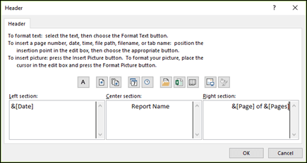
To add or change the header or footer text, type additional text or edit the existing text in the Left, Center, or Right section box.
To start a new line in a header or footer text box, press Enter.
To include a single ampersand (&) in the text of a header or footer, use two ampersands. For example, to include «Subcontractors & Services» in a header, type Subcontractors && Services.
Excel has many built-in text headers and footers that you can use. For worksheets, you can work with headers and footers in Page Layout view. For chart sheets or charts you need to go through the Page Setup dialog.
Click the worksheet where you want to add or change a built-in header or footer.
On the Insert tab, in the Text group, click Header & Footer.
Excel displays the worksheet in Page Layout view.
Click the left, center, or right header or the footer text box at the top or the bottom of the worksheet page.
Tip: Clicking any text box selects the header or footer and displays the Header and Footer Tools, adding the Design tab.
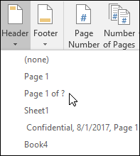
On the Design tab, in the Header & Footer group, click Header or Footer, and then click the built-in header or footer that you want.
Instead of picking a built-in header or footer, you can choose a built-in element. Many elements (such as Page Number, File Name, and Current Date) are found on the ribbon. For worksheets, you can work with headers and footers in Page Layout view. For chart sheets or charts, you can work with headers and footers in the Page Setup dialog.
Click the worksheet to which you want to add specific header or footer elements.
On the Insert tab, in the Text group, click Header & Footer.
Excel displays the worksheet in Page Layout view.
Click the left, center, or right header or footer text box at the top or the bottom of the worksheet page.
Tip: Clicking any text box selects the header or footer and displays the Header and Footer Tools, adding the Design tab.
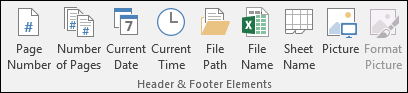
On the Design tab, in the Header & Footer Elements group, click the elements that you want.
Click the chart sheet or chart where you want to add or change a header or footer element.
On the Insert tab, in the Text group, click Header & Footer.
Excel displays the Page Setup dialog box.
Click Custom Header or Custom Footer.
Use the buttons in the Header or Footer dialog box to insert specific header and footer elements.
Tip: When you rest the mouse pointer on a button, a ScreenTip displays the name of the element that the button inserts.
For worksheets, you can work with headers and footers in Page Layout view. For chart sheets or charts, you can work with headers and footers in the Page Setup dialog.
Click the worksheet where you want to choose header and footer options.
On the Insert tab, in the Text group, click Header & Footer.
Excel displays the worksheet in Page Layout view.
Click the left, center, or right header or footer text box at the top or the bottom of the worksheet page.
Tip: Clicking any text box selects the header or footer and displays the Header and Footer Tools, adding the Design tab.
On the Design tab, in the Options group, check one or more of the following:
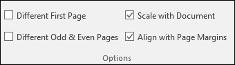
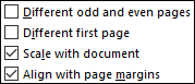
To remove headers and footers from the first printed page, select the Different First Page check box.
To specify that the headers and footers on odd-numbered pages should differ from those on even-numbered pages, select the Different Odd & Even Pages check box.
To specify whether the headers and footers should use the same font size and scaling as the worksheet, select the Scale with Document check box.
To make the font size and scaling of the headers or footers independent of the worksheet scaling, which helps create a consistent display across multiple pages, clear this check box.
To make sure the header or footer margin is aligned with the left and right margins of the worksheet, select the Align with Page Margins check box.
To set the left and right margins of the headers and footers to a specific value that is independent of the left and right margins of the worksheet, clear this check box.
Click the chart sheet or chart where you want to choose header or footer options.
On the Insert tab, in the Text group, click Header & Footer.
Excel displays the Page Setup dialog box.
Select one or more of the following:
To remove headers and footers from the first printed page, select the Different first page check box.
To specify that the headers and footers on odd-numbered pages should differ from those on even-numbered pages, select the Different odd & even pages check box.
To specify whether the headers and footers should use the same font size and scaling as the worksheet, select the Scale with document check box.
To make the font size and scaling of the headers or footers independent of the worksheet scaling, which helps create a consistent display across multiple pages, clear the Scale with Document check box.
To guarantee that the header or footer margin is aligned with the left and right margins of the worksheet, select the Align with page margins check box.
Tip: To set the left and right margins of the headers and footers to a specific value that is independent of the left and right margins of the worksheet, clear this check box.
To close the header and footer, you must switch from Page Layout view to Normal view.
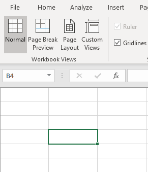
On the View tab, in the Workbook Views group, click Normal.
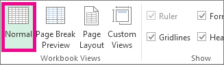
You can also click Normal  on the status bar.
On the Insert tab, in the Text group, click Header & Footer.
Excel displays the worksheet in Page Layout view.
Click the left, center, or right header or the footer text box at the top or the bottom of the worksheet page.
Tip: Clicking any text box selects the header or footer and displays the Header and Footer Tools, adding the Design tab.
Press Delete or Backspace.
Note: If you want to delete headers and footers for several worksheets at once, select the worksheets, and then open the Page Setup dialog box. To delete all headers and footers instantly, on the Header/Footer tab, select (none) in the Header or Footer box.
Need more help?
You can always ask an expert in the Excel Tech Community or get support in the Answers community.
Источник
Excel for Microsoft 365 Excel for Microsoft 365 for Mac Excel 2021 Excel 2021 for Mac Excel 2019 Excel 2019 for Mac Excel 2016 Excel 2016 for Mac Excel 2013 Excel 2010 Excel 2007 More…Less
To make managing and analyzing a group of related data easier, you can turn a range of cells into an Excel table (previously known as an Excel list).
Note: Excel tables should not be confused with the data tables that are part of a suite of what-if analysis commands. For more information about data tables, see Calculate multiple results with a data table.
Learn about the elements of an Excel table
A table can include the following elements:
-
Header row By default, a table has a header row. Every table column has filtering enabled in the header row so that you can filter or sort your table data quickly. For more information, see Filter data or Sort data.

You can turn off the header row in a table. For more information, see Turn Excel table headers on or off.
-
Banded rows Alternate shading or banding in rows helps to better distinguish the data.
-
Calculated columns By entering a formula in one cell in a table column, you can create a calculated column in which that formula is instantly applied to all other cells in that table column. For more information, see Use calculated columns in an Excel table.
-
Total row Once you add a total row to a table, Excel gives you an AutoSum drop-down list to select from functions such as SUM, AVERAGE, and so on. When you select one of these options, the table will automatically convert them to a SUBTOTAL function, which will ignore rows that have been hidden with a filter by default. If you want to include hidden rows in your calculations, you can change the SUBTOTAL function arguments.
For more information, also see Total the data in an Excel table.
-
Sizing handle A sizing handle in the lower-right corner of the table allows you to drag the table to the size that you want.
For other ways to resize a table, see Resize a table by adding rows and columns.
Create a table
You can create as many tables as you want in a spreadsheet.
To quickly create a table in Excel, do the following:
-
Select the cell or the range in the data.
-
Select Home > Format as Table.
-
Pick a table style.
-
In the Format as Table dialog box, select the checkbox next to My table as headers if you want the first row of the range to be the header row, and then click OK.
Also watch a video on creating a table in Excel.
Working efficiently with your table data
Excel has some features that enable you to work efficiently with your table data:
-
Using structured references Instead of using cell references, such as A1 and R1C1, you can use structured references that reference table names in a formula. For more information, see Using structured references with Excel tables.
-
Ensuring data integrity You can use the built-in data validation feature in Excel. For example, you may choose to allow only numbers or dates in a column of a table. For more information on how to ensure data integrity, see Apply data validation to cells.
Export an Excel table to a SharePoint site
If you have authoring access to a SharePoint site, you can use it to export an Excel table to a SharePoint list. This way other people can view, edit, and update the table data in the SharePoint list. You can create a one-way connection to the SharePoint list so that you can refresh the table data on the worksheet to incorporate changes that are made to the data in the SharePoint list. For more information, see Export an Excel table to SharePoint.
Need more help?
You can always ask an expert in the Excel Tech Community or get support in the Answers community.
See Also
Format an Excel table
Excel table compatibility issues
Need more help?
Want more options?
Explore subscription benefits, browse training courses, learn how to secure your device, and more.
Communities help you ask and answer questions, give feedback, and hear from experts with rich knowledge.
As a user, it’s easy to get lost when tracking the meaning of values. What’s more, Excel Printouts don’t have row numbers or column letters. Learning how to create a header row in excel is the ultimate solution to save you hours of work.
Usually, working with multiple pages can be confusing since they have no labels. Consequently, you are left wondering what each row represents in your spreadsheet.
In this guide, you will learn how to add an excel header row by printing or freezing header rows. So, you needn’t get lost anymore when tracking the values of multiple pages.
Creating Header Rows in Excel
Let’s dive into different methods to achieve creating header rows in Microsoft excel.
Method 1: Repeat Header Row across Multiple Spreadsheets by Printing
Assuming you want to print an excel document that spans different pages. However, on printing, you get the shock of your life that only one page has column titles. Relax. Change the settings in the Page Set-up to repeat the top header row in excel for every page.
Here’s how to repeat header row in Excel:
- First, open the Excel worksheet that needs printing.
- Navigate to the Page Layout Menu.
- In the Page Set-Up group, now click on Print Titles.
- The Print title command is inactive or dim if you are editing a cell. What’s more, selecting a chart in the same worksheet also dims this command.
- Alternatively, click on the Page Set-up arrow button below the Print Titles.
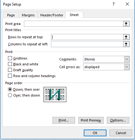
- Click on the Sheet tab from the Page Setup dialogue box.

- Under the print titles section, identify the Rows to repeat at the top section
- Ensure that you select only one workbook to repeat the headers. Otherwise, if you have several worksheets, the Rows to repeat at top and Columns to repeat at left section are invisible or greyed out.
- Click in the Rows to repeat at the top section
- Now, click on the excel header row in your spreadsheet that you want to repeat
- The Rows to repeat at top field formula is generated as shown belowAlternatively,
- Click on the Collapse Dialog icon next to the Rows to repeat at the top section.
Now, this action minimizes the page setup window, and you can resume to the worksheet. - Select the header rows that you want to repeat using the black cursor with one click
- After that, click the Collapse Dialog icon or ENTER to return to the Page Setup dialogue box.
- Click on the Collapse Dialog icon next to the Rows to repeat at the top section.
The selected rows are now displayed in the Rows to repeat at the top field, as shown below.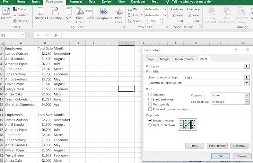
- Now, click on the Print Preview at the bottom of the Page Setup dialogue box.
- If you are happy with the results, click OK.
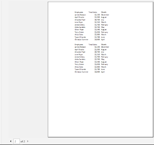
The header rows will be repeated on all pages of your worksheet when you print as shown in the images below.

Good job! Now you are an expert on how to repeat header rows in excel.
Method 2: Freezing Excel Header Row
You can create header rows by freezing them. That way, the row headers stay in place as you scroll down the rest of the spreadsheet.
- First, open your desired spreadsheet
- Next, click the View tab and select Freeze Panes
- Click on Freeze Top from the drop-down menu
Automatically, the top row, which is the row headings, is frozen as indicated by the grey gridlines. When you scroll down or up, the header rows remain in place.
Alternatively,
- Open your excel spreadsheet
- Click on the row below your header rows
- Navigate to the View tab
- Click on Freeze Panes
- From the drop-down menu, select Freeze Panes
Excel automatically locks the header row by displaying a grey line on the gridlines. That way, your row headers remain visible in the entire spreadsheet.
Method 3: Format your Spreadsheet as a Table with Header Rows
Creating header rows reduces confusion when trying to figure out what each row represents. To format your sheet as a table with row headings, here’s what you need to do:
- First, select all the data in your spreadsheet
- Next, click on the Home Tab
- Navigate to Format as Table ribbon. Select your desired style, either light, medium, or dark.
- The Format As Table dialogue box appears
- Now, confirm whether the cells represent the right data for your table
- Make sure that you tick My table has headers checkbox
- Click OK.

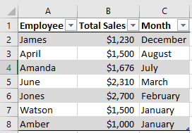
You have successfully created a table that contains header rows. As a result, it is easy to handle data efficiently without getting confused or losing sight of valuable information.
How to Disable Excel Table Headers
Now that you have formatted your spreadsheet as a table with header rows, it’s possible to disable them. Here’s how:
- First, open your spreadsheet.
- Next, click on the Design tab on the toolbar.
- Uncheck Header Row box under the Table Styles Option
This process turns off the visibility of row headers on your spreadsheet.
A spreadsheet that lacks header rows is bound to create confusion. What’s more, it leaves you second-guessing values and reduces data efficiency. Nevertheless, you can create excel header rows by repeating header, freezing, or formatting as tables when handling valuable data. Click here to learn how to merge cells in excel.