
Excel for Microsoft 365 Excel for Microsoft 365 for Mac Excel for the web Excel 2021 Excel 2021 for Mac Excel 2019 Excel 2019 for Mac Excel 2016 Excel 2016 for Mac Excel 2013 Excel 2010 Excel for Mac 2011 Excel Mobile More…Less
Managing personal finances can be a challenge, especially when trying to plan your payments and savings. Excel formulas and budgeting templates can help you calculate the future value of your debts and investments, making it easier to figure out how long it will take for you to reach your goals. Use the following functions:
-
PMT calculates the payment for a loan based on constant payments and a constant interest rate.
-
NPER calculates the number of payment periods for an investment based on regular, constant payments and a constant interest rate.
-
PV returns the present value of an investment. The present value is the total amount that a series of future payments is worth now.
-
FV returns the future value of an investment based on periodic, constant payments and a constant interest rate.
Figure out the monthly payments to pay off a credit card debt
Assume that the balance due is $5,400 at a 17% annual interest rate. Nothing else will be purchased on the card while the debt is being paid off.
Using the function PMT(rate,NPER,PV)
=PMT(17%/12,2*12,5400)
the result is a monthly payment of $266.99 to pay the debt off in two years.
-
The rate argument is the interest rate per period for the loan. For example, in this formula the 17% annual interest rate is divided by 12, the number of months in a year.
-
The NPER argument of 2*12 is the total number of payment periods for the loan.
-
The PV or present value argument is 5400.
Figure out monthly mortgage payments
Imagine a $180,000 home at 5% interest, with a 30-year mortgage.
Using the function PMT(rate,NPER,PV)
=PMT(5%/12,30*12,180000)
the result is a monthly payment (not including insurance and taxes) of $966.28.
-
The rate argument is 5% divided by the 12 months in a year.
-
The NPER argument is 30*12 for a 30 year mortgage with 12 monthly payments made each year.
-
The PV argument is 180000 (the present value of the loan).
Find out how to save each month for a dream vacation
You’d like to save for a vacation three years from now that will cost $8,500. The annual interest rate for saving is 1.5%.
Using the function PMT(rate,NPER,PV,FV)
=PMT(1.5%/12,3*12,0,8500)
to save $8,500 in three years would require a savings of $230.99 each month for three years.
-
The rate argument is 1.5% divided by 12, the number of months in a year.
-
The NPER argument is 3*12 for twelve monthly payments over three years.
-
The PV (present value) is 0 because the account is starting from zero.
-
The FV (future value) that you want to save is $8,500.
Now imagine that you are saving for an $8,500 vacation over three years, and wonder how much you would need to deposit in your account to keep monthly savings at $175.00 per month. The PV function will calculate how much of a starting deposit will yield a future value.
Using the function PV(rate,NPER,PMT,FV)
=PV(1.5%/12,3*12,-175,8500)
an initial deposit of $1,969.62 would be required in order to be able to pay $175.00 per month and end up with $8500 in three years.
-
The rate argument is 1.5%/12.
-
The NPER argument is 3*12 (or twelve monthly payments for three years).
-
The PMT is -175 (you would pay $175 per month).
-
The FV (future value) is 8500.
Find out how long it will take to pay off a personal loan
Imagine that you have a $2,500 personal loan, and have agreed to pay $150 a month at 3% annual interest.
Using the function NPER(rate,PMT,PV)
=NPER(3%/12,-150,2500)
it would take 17 months and some days to pay off the loan.
-
The rate argument is 3%/12 monthly payments per year.
-
The PMT argument is -150.
-
The PV (present value) argument is 2500.
Figure out a down payment
Say that you’d like to buy a $19,000 car at a 2.9% interest rate over three years. You want to keep the monthly payments at $350 a month, so you need to figure out your down payment. In this formula the result of the PV function is the loan amount, which is then subtracted from the purchase price to get the down payment.
Using the function PV(rate,NPER,PMT)
=19000-PV(2.9%/12, 3*12,-350)
the down payment required would be $6,946.48
-
The $19,000 purchase price is listed first in the formula. The result of the PV function will be subtracted from the purchase price.
-
The rate argument is 2.9% divided by 12.
-
The NPER argument is 3*12 (or twelve monthly payments over three years).
-
The PMT is -350 (you would pay $350 per month).
See how much your savings will add up to over time
Starting with $500 in your account, how much will you have in 10 months if you deposit $200 a month at 1.5% interest?
Using the function FV(rate,NPER,PMT,PV)
=FV(1.5%/12,10,-200,-500)
in 10 months you would have $2,517.57 in savings.
-
The rate argument is 1.5%/12.
-
The NPER argument is 10 (months).
-
The PMT argument is -200.
-
The PV (present value) argument is -500.
See also
PMT function
NPER function
PV function
FV function
Need more help?
This tutorial will demonstrate various ways to calculate compound interest in Excel and Google Sheets.
What is Compound Interest?
When you invest money, you can earn interest on your investment. Say, for example, you invest $3,000 with a 10% annual interest rate, compounded annually. One year from the initial investment (called the principal), you earn $300 ($3,000 x 0.10) in interest, so your investment is worth $3,300 ($3,000 + $300). For the next period, you earn interest based on the gross figure from the previous period: $330 ($3,300 x 0.10) because your investment was worth $3,300. Now, it is worth $3,630.
The general formula for compound interest is: FV = PV(1+r)n, where FV is future value, PV is present value, r is the interest rate per period, and n is the number of compounding periods.
How to Calculate Compound Interest in Excel
One of the easiest ways is to apply the formula: (gross figure) x (1 + interest rate per period).
If you are investing $1,000 with a 15% interest rate, compounded annually, below is how you would calculate the value of your investment after one year.
= B2 * (1 + $A2)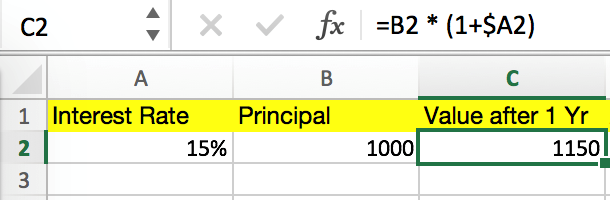
In this case B2 is the Principal, and A2 is the Interest Rate per Period. The “$” is used in the formula to fix the reference to column A, since the interest rate is constant in this example.
You can calculate the value of your investment after two years by simply copying and pasting the formula into cell D2, as shown below.
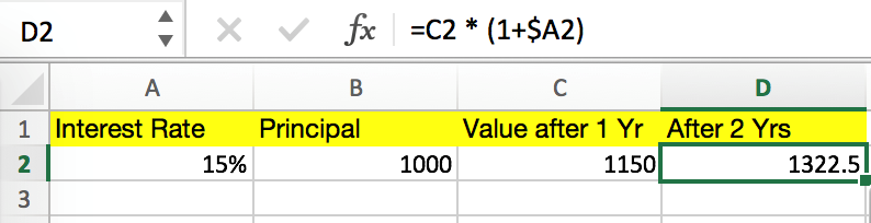
C2 is the current gross figure. Notice how B2 automatically changes to C2, since the cell reference has changed. You could copy the formula over additional columns to calculate the compounded value in future years. We would recommend structuring a table like this (vertically instead of horizontally):
Rolling Total Compound Interest Table
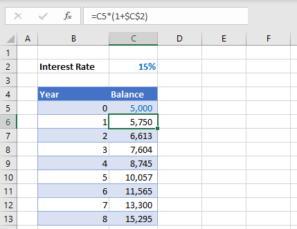
The process above for calculating compound interest is easy, but if you want to figure out the value of your investment after 10 years, for example, this process is not efficient. Instead you could use a generalized compound interest formula.
General Compound Interest Formula (for Daily, Weekly, Monthly, and Yearly Compounding)
A more efficient way of calculating compound interest in Excel is applying the general interest formula: FV = PV(1+r)n, where FV is future value, PV is present value, r is the interest rate per period, and n is the number of compounding periods.
Say, for instance that you are investing $5,000 with a 10% annual interest rate, compounded semi-annually, and you want to figure out the value of your investment after five years. The spreadsheet below shows how this calculation can be done on Excel.
= B1 * (1 + $B2/2)^(B3 * B4)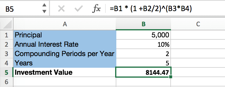
In this case, PV is the Principal, r is (Annual Interest Rate) / 2 because interest is compounded semi-annually (twice per year), n is (Compounding Periods per Year) x (Year), and FV is the Investment Value. This process is more efficient than the first one because you don’t have to calculate the gross figure after each period, saving quite a few calculation steps.
FV Function and Compound Interest
Lastly, you can calculate compound interest with Excel’s built-in Future Value Function. Similar to the previous process, the FV function calculates the future value of an investment based on the values of certain variables.
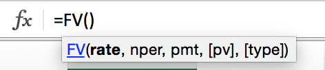
The variables (as shown above) are:
– rate is the interest rate for each period.
– nper is the number of compounding periods.
– pmt is the additional payment per period, and it is represented as a negative number. If there is no value for “pmt,” put a value of zero.
– pv (optional) is the principal investment, which is also represented as a negative number. If there is no value for “pv,” you must include a value for “pmt.”
– type (optional) indicates when additional payments occur. “0” indicates that the payments occur in the beginning of the period, and “1” indicates that the payments are due at the end of the period.
The previous semi-annual compound interest example can be completed with the FV function.
= FV(B2 / B3, B3 * B4, 0, -B1)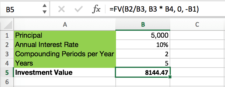
The “rate” is (Annual Interest Rate) / (Compounding Period per Year), “nper” is (Compounding Periods per Year) x (Years), “pmt” is 0, and “pv” is – (Principal).
Understanding how to calculate compound interest is important for predicting investment performance, whether it’s for retirement planning or your personal portfolio, and Excel is an excellent tool to do so.
For more information about Compound Interest visit Investopedia
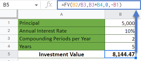
Calculate Compound Interest in Google Sheets
These formulas work exactly the same in Google Sheets as in Excel.
![]()
Download Article
![]()
Download Article
This wikiHow teaches you how to create an interest payment calculator in Microsoft Excel. You can do this on both Windows and Mac versions of Excel.
-

1
Open Microsoft Excel. Double-click the Excel app icon, which resembles a white «X» on a dark-green background.
-
2
Click Blank Workbook. It’s in the upper-left side of the main Excel page. Doing so opens a new spreadsheet for your interest calculator.
- Skip this step on Mac.
Advertisement
-
3
Set up your rows. Enter your payment headings in each of the following cells:
- Cell A1 — Type in Principal
- Cell A2 — Type in Interest
- Cell A3 — Type in Periods
- Cell A4 — Type in Payment
-
4
Enter the payment’s total value. In cell B1, type in the total amount you owe.
- For example, if you bought a boat valued at $20,000 for $10,000 down, you would type 10,000 into B1.
-
5
Enter the current interest rate. In cell B2, type in the percentage of the interest that you have to pay each period.
- For example, if your interest rate is three percent, you would type 0.03 into B2.
-
6
Enter the number of payments you have left. This goes in cell B3. If you’re on a 12-month plan, for example, you would type 12 into cell B3.
-
7
Select cell B4. Simply click B4 to select it. This is where you’ll enter the formula to calculate your interest payment.
-
8
Enter the interest payment formula. Type
=IPMT(B2, 1, B3, B1)into cell B4 and press ↵ Enter. Doing so will calculate the amount that you’ll have to pay in interest for each period.- This doesn’t give you the compounded interest, which generally gets lower as the amount you pay decreases. You can see the compounded interest by subtracting a period’s worth of payment from the principal and then recalculating cell B4.


Advertisement
Add New Question
-
Question
The interest is 6% per annum, and the amount deposited is 500,000 on January 2016. If a member withdraws his amount on May 2016, what is the interest?

6% per annum is .5% monthly (.5 * 12 = 6), so that’s $2500.00 in interest per month ($500,000 *.5% = $2,500, or $500,000 * .005 = $2,500). If the member withdrew in May before the interest was calculated and paid out for the month of May, then $10,000.00 ($2,500 * 4) in interest. If after, then $12,500.00 ($2,500 * 5) in interest.
Ask a Question
200 characters left
Include your email address to get a message when this question is answered.
Submit
Advertisement
Video
-
You can copy and paste cells A1 through B4 into another part of the spreadsheet in order to evaluate the changes made by different interest rates and terms without losing your original formula and result.
Thanks for submitting a tip for review!
Advertisement
-
Interest rates are subject to change. Make sure you read the fine print on your interest agreement before you calculate your interest.
Advertisement
About This Article
Article SummaryX
1. Label rows for Principal, Interest, Periods, and Payment.
2. Enter total value in the Principal row.
3. Enter the interest rate into the Interest row.
4. Enter the amount of remaining payments in the Periods row.
5. Click the first blank cell in the Payments row.
6. Type » =IPMT(B2, 1, B3, B1)» into the cell.
7. Press Enter.
Did this summary help you?
Thanks to all authors for creating a page that has been read 502,521 times.
Is this article up to date?
Summary
To calculate simple interest in Excel (i.e. interest that is not compounded), you can use a formula that multiples principal, rate, and term.
This example assumes that $1000 is invested for 10 years at an annual interest rate of 5%. Simple interest means that interest payments are not compounded – the interest is applied to the principal only.
In the example shown, the formula in C8 is:
=C5*C7*C6
Generic formula
interest=principal*rate*termExplanation
The general formula for simple interest is:
interest=principal*rate*term
So, using cell references, we have:
=C5*C7*C6
=1000*10*0.05
=500

Author![]()
Dave Bruns
Hi — I’m Dave Bruns, and I run Exceljet with my wife, Lisa. Our goal is to help you work faster in Excel. We create short videos, and clear examples of formulas, functions, pivot tables, conditional formatting, and charts.
Related Information
I just wanted to say thanks for simplifying the learning process for me! Your website is a life saver!
Get Training
Quick, clean, and to the point training
Learn Excel with high quality video training. Our videos are quick, clean, and to the point, so you can learn Excel in less time, and easily review key topics when needed. Each video comes with its own practice worksheet.
View Paid Training & Bundles
Help us improve Exceljet
Excel — is the versatile analytical and computational tool that is often used by lenders (banks, investors, etc.) and borrowers (businessmen, companies, private persons, etc.).
Quickly navigate in the intricate formulas, calculate to interest, payouts, overpayment to allow Microsoft Excel program functions.
How to calculate credit payments in Excel
Monthly payments depend on the loan repayment scheme. There are annuity and differentiated payments:
- The annuity assumes that the client makes each month the same amount.
- When the differentiated scheme of repayment of debt before the financial organization interest is charged on the balance of the loan amount. Therefore, the monthly payments will be reduced.
Increasingly used annuity: it`s more profitable for the bank, and it is more convenient for the majority of customers.
The calculation of annuity payments on the loan in Excel
The monthly annuity payment is calculated as follows:
S = C * V
where:
- S – sum, is the payment amount on the loan;
- C – coefficient, is the annuity payment rate;
- V – is the value of the loan.
The annuity factor Formula:
С = (i * (1 + i) ^ n) / ((1 + i) ^ n-1)
- where is i – the interest rate for the month, the result of dividing the annual rate by 12;
- n – is the loan term in months.
There is a special feature in Excel which said to the annuity payments. This is: =PMT().
- Fill in the input data for calculating the monthly payments on the credit. This is loan amount, interest and term.
- To make the repayment schedule. It`s empty till.
- In the first cell of the column «Credit payments», introduced the formula of the calculating the loan annuity payments in Excel: =PMT($B$3/12,$B$4,$B$2). To fix the cells, are used to the absolute links. In the formula may be administered directly to the numbers and not the reference cell data. Then it will have the following form: =PMT(18%/12,36,100000).
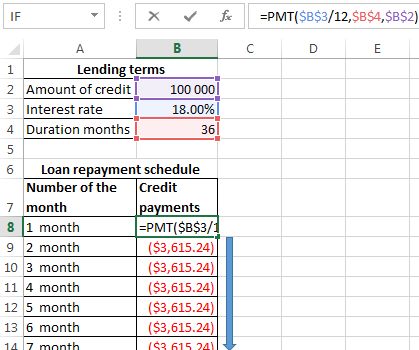
The cells turned into red, because we’ll give these money to the bank and to lose the money.
The calculation of payments in Excel for the differentiated scheme of repayment
The differentiated payment method implies that:
- the principal amount is distributed over the period of payment in the equal installments;
- the loan interest accrued on the balance.
The formula for the calculating to the differential payment:
DP = NEO / (PP + PS * NEO)
where:
- DP – is the monthly payment on the loan;
- NEO – is the loan balance;
- PP – the number of remaining until the end of the repayment period;
- PS – is the interest rate per month (the annual rate divided by 12).
Draw up the schedule for repayment of the previous loan on the differentiated scheme.
The input dates are the same:
| Lending terms | |
| Amount of credit | $100 000 |
| Interest rate | 18% |
| Duration months | 36 |
To make the schedule of repayment of the loan:
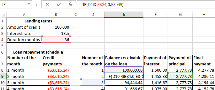
| Number of the month | Balance receivable on the loan | Payment of interest | Payment of principal | Final payment |
| 1 month |
Balance receivable on the loan: in the first month it is equal to the entire amount =$B$2. In the second one and in the subsequent ones — calculated by the formula: =IF(D10>$B$4,0,E8-G9). Where is:
- D10 – the number of the current period;
- $B$4 – is the term of the loan;
- E8 – is the balance of the loan in the previous period;
- G9 — is the principal debt in the previous period.
Payment of interest: the balance of the loan in the current period multiplied by the monthly interest rate / 12 months: =E9*($B$3/12).
Payment of principal: the amount of the loan divided by the period: =IF(D9<=$B$4,$B$2/$B$4,0).
Final payment: the sum of «the interest» and «the main debt» in the current period: =F8+G8.
We substitute to the formulas in the corresponding columns. Copy them to the entire table.
To compare the overpayment on the annuity and the differentiated scheme of the repayment on credit:
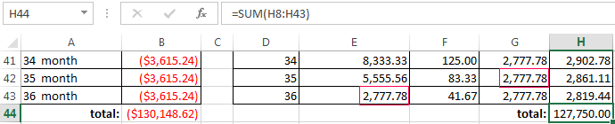
The red figure – is the annuity (was taken 100 000 rubles), the black one – is the differentiated way.
Interest calculation formula for loans in Excel
The calculation of interest on the loan in Excel and calculate the effective interest rate, with the following information on the bank offers credit:
We carry out interest calculation on loan and calculate the effective interest rate with the following information on the bank offers credit.
Fill in the table type:
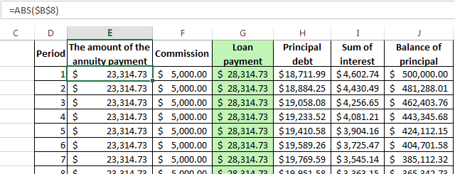
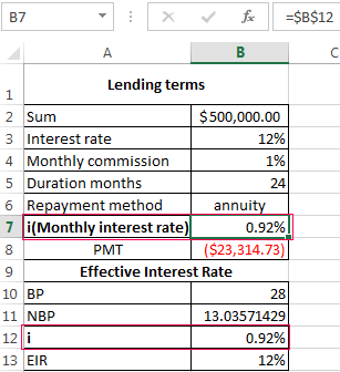
The commission is taken monthly from the whole sum. The total loan payment — this is the annuity payment plus the commission. The sum of the main debt and the sum of interest – there are components parts of the annuity payment.
The principal amount = the annuity payment – the interest.
The sum of interest = the remaining debt * the monthly interest rate.
The balance of principal = the residue of the previous period – the sum of the principal debt in the previous period.
Based on the table of monthly payments, calculate the effective interest rate:
- took the credit 500 000 rubles;
- returned to the bank — 684 881. 67 rubles (the sum of all payments on the loan);
- the overpayment was 184 881. 67 rubles;
- the interest rate — 184 881 67/500 000 * 100, or 37%.
- the harmless commission of 1% was cost for the borrower so expensive.
The effective interest rate of the loan without the commission will be 13%. The counting is carried out in the same way.
The calculation of effective interest rate in Excel
According to the law about the consumer credit for the calculation of the effective interest rate now is applied the new formula. EIR (Effective Interest Rate) is defined in percentage of up to the third decimal place according to the following formula:
- EIR = i * CHBP * 100;
- where is i — the interest rate of the base period;
- NBP — the number of base periods in a calendar year.
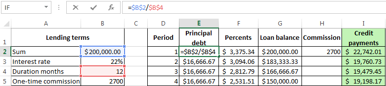
Take for example the following dates on the loan:
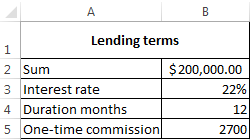
For calculating of the effective interest rate is necessary to make a payment schedule (see the order above).
It is necessary to determine the base period (BP). The law states that this is the standard time interval, which is found in most of the repayment schedule. Example BP = 28 days.
Then we find NBP: 365/28 = 13.
Now you can find the interest rate of the base period:
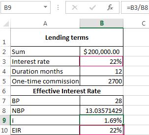
We have all the necessary dates — substitute them in the EIR formula: =B9*B8
To obtain the percentages in Excel, you do not need to multiple by 100. It is enough to set for the cell with the result to the percentage format.
EIR for the new formula is coincided with the annual interest rate on the loan.
Download credit calculator in Excel
Thus, for calculating the annuity payments on the loan is used the simplest function PLT. As you can see, the differentiated way of repayment is a bit more complicated.
There is a formula in Excel which calculates simple interest by multiplying the principal, the rate, and the term.
Calculate simple interest in Excel
Consider the example demonstrated below in which the formula in C5 is =C2*C3*C4
In order to do a simple interest calculation in Excel using the COUNTA function, follow the procedure below:
- Click on Formulas on the menu bar in Excel.
- Next, click on More Functions and point the cursor on Statistical.
- Scroll down the list that displays and click on COUNTA.
The dialogue box will display as shown below.
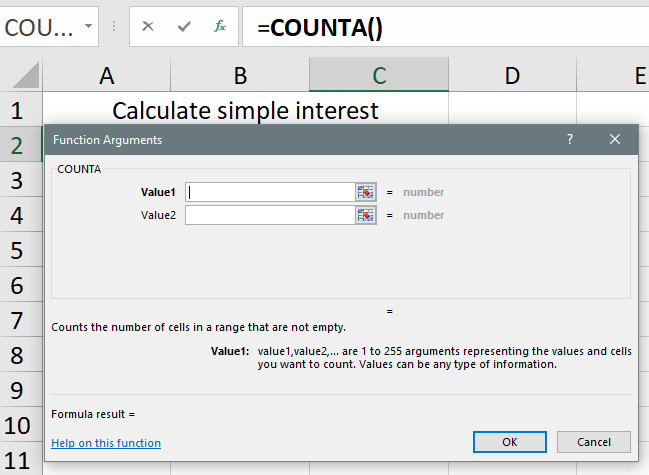
Figure 1. How to access COUNTA formula in Excel
Example 1
- The value 1 represents the span of cells to which you want to apply the formula. In the example below, it is C2 to C4. Type C2:C4.
- Click on OK.
It will show you the result displayed in the screenshot below:
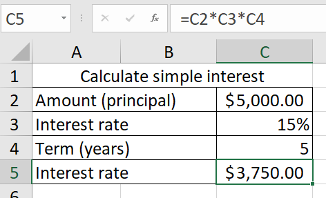 Figure 2. The result displayed by COUNTA
Interpretation of the Result
What is displayed above shows that for a given amount of money (principal), say $5000, invested at the interest rate of 5 percent per year for 15 years, using the COUNTA function to calculate the interest generated, that is, =C2*C3*C4 the answer is $3,750. It is possible to verify this formula by manually doing the calculation as shown below:
Interest = Amount X Rate X Term
= 5000X0.05X15
= 3,750.
Alternatively, you can still calculate the simple interest by simply typing the formula above into the cell on the right of the row you are interested in. Hit the enter key when you finish typing, and the result will show.
The General Formula
The general formula for calculating simple interest in Excel is shown below:
Interest = Principal*Rate*Term
This means that you have to multiply the principal by the rate and by the term.
In the example demonstrated above, the amount of $5000 is invested at the rate of 5% per annum for a period of 15 years. The formula imputed into C5 is
=C2*C3*C4
Example 2
Calculate the simple interest on $3000 invested at the rate of 10% per annum for 2 years using Excel.
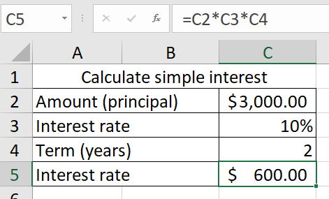
Figure 3. Simple interest on $3000 invested at the rate of 10% per annum for 2 years
The same principle applies. In this example, the formula in C5 is
=C2*C3*C4
It can also be verified by doing the calculation physically as shown below:
Interest = Amount X Rate X Years
= 3000 X 10 X 2
= 600.
Example 3
Calculate the simple interest on $500 invested at the rate of 6% per annum for 10 years using Excel.
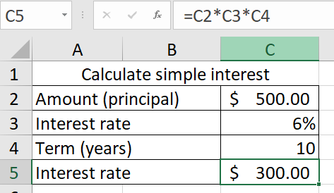
Figure 4. Simple interest on $500 invested at the rate of 6% per annum for 10 years
In the example above, the formula in C5 is
=C2*C3*C4
However, because the values are different, the interest calculated is different also. This too can also be verified by doing the calculation physically as shown below:
Interest = Amount X Rate X Years
= 500 X 6 X 10
= 300.
Still need some help with Excel formatting or have other questions about Excel? Connect with a live Excel expert here for some 1 on 1 help. Your first session is always free.
In this article, we will learn how to use Simple interest formula in Excel.
Calculate the simple interest amount given the present or principal amount, rate in annum & period in years.
Syntax:
=PA * rate * period
PA : principal amount
Rate : Rate per annum
Period : Period in years
Let’s understand this function using an example.
Here we have a data set and to get Simple interest(SI) amount
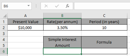
We need to find the simple interest amount for the dateset.
Use the formula to get the simple interest amount
=A2 * B2 * C2
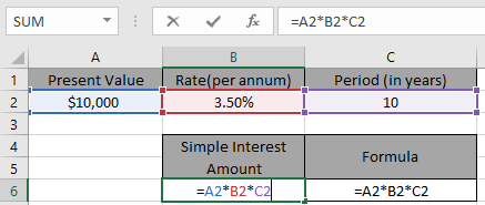
Press Enter

As you can see the simple interest amount for the dataset is $ 3500.
Note: Remember to keep the data in term of years.
Hope you understood how to get the simple interest amount in Excel. Explore more articles on Excel statistical function here. Please feel free to state your query or feedback for the above article.
Related Articles:
Excel IPMT Function
How to use Compound Interest Function in Excel
Popular Articles:
50 Excel Shortcuts to Increase Your Productivity
How to use the VLOOKUP Function in Excel
How to use the COUNTIF function in Excel
How to use the SUMIF Function in Excel
Compound interest is one of the most important financial calculations that most of us often use, and it’s a must to learn to calculate it in Excel.
But before you do that you need to understand what actually compound interest is.
Compound interest is interest calculated on the initial principal and also on the accumulated interest of previous periods of a deposit or loan.
Investopedia
In Excel, the method to calculate compound interest is simple.
Now, the thing is. You just need to use a calculation method and specify the time period for which you want to calculate.
So today, in this post, I’d like to show you how to calculate compound interest in Excel using different time periods. So let’s get started.
Yearly Compound Interest Formula
For calculating yearly compound interest, you just have to add the interest of the one year into next year’s principal amount to calculate the interest of the next year.
And, the formula in excel for yearly compound interest will be.
=Principal Amount*((1+Annual Interest Rate/1)^(Total Years of Investment*1)))Let me show you an example.

In the above example, with $10000 of principal amount and 10% interest for 5 years, you will get $16105.
In the first year, you will get $10000*10% which is $1000, and in the second year, ($10000+$1000)*10% = $1100, and so on.
Quarterly Compound Interest Formula
Calculating quarterly compound interest is just like calculating yearly compound interest.
But, here you need to calculate interest four times a year. The interest amount for each quarter will add to the principal amount for the next quarter. To calculate the quarterly compound interest you can use the below-mentioned formula.
=Principal Amount*((1+Annual Interest Rate/4)^(Total Years of Investment*4)))Here is an example.

In the above example, with $10000 of principal amount and 10% interest for 5 years, we will get $16386.
In the first quarter, we get 10000*(10%/4) which is $250, and in the second quarter, ($10000+$250)*(10%/4) = $256, and the same calculation method for 20 Quarters (5 years).
Monthly Compound Interest Formula
While calculating the monthly compound interest you need to use the basis you have used in other time periods.
You have to calculate the interest at the end of each month. And, in this method interest rate will divide by 12 for a monthly interest rate. To calculate the monthly compound interest in Excel, you can use the below formula.
=Principal Amount*((1+Annual Interest Rate/12)^(Total Years of Investment*12)))
In the above example, with $10000 of principal amount and 10% interest for 5 years, we will get $16453.
In the first month, we get 10000*(10%/12) which is $83.33 & in the second month, ($10000+$83.33)*(10%/12) = $84.02 and the same is for 60 months (5 years).
Daily Compound Interest Formula
While calculating daily compound interest again we have to use the same method with the below calculation formula. We have to divide the interest rate by 365 to get a daily interest rate.
So, you can use the below formula to calculate daily compound interest.
=Principal Amount*((1+Annual Interest Rate/365)^(Total Years of Investment*365)))
In the above example, with $10000 of principal amount and 10% interest for 5 years, we will get $16486.
On the first day, we get 10000*(10%/365) which is $4, and on the second day, ($10000+$4)*(10%/365) = $4, and the same is for every day for 5 years.
Sample File
By using the above methods, I have created a cumulative interest calculator [Template] to calculate all of the above calculations for interest in a single worksheet.
sample-files.xlsx
More Formulas
- Calculate Cube Root in Excel
- Calculate Percentage Variance (Difference)
- Calculate Simple Interest in Excel
- Calculate SQUARE ROOT in Excel
- Calculate the Weighted Average in Excel
- Does Not Equal Operator in Excel
- Round a Number to Nearest 1000, 100, and 10
- Round to Nearest .5, 5. 50 (Down-Up) in Excel
- Square a Number in Excel
- Round a Number to Nearest 1000 in Excel
- Add-Subtract Percentage from a Number
- Average But Ignore Errors
- Average Number but Exclude Zeros
- Average Only Non-Blank Cells
- Calculate the Average of the Percentage Values
- Calculate the Average of the Time Values
- Calculate the Cumulative Sum of Values
- Round Percentage Values
⇠ Back to 100+ Excel Formulas List (Basic + Advanced)
Compound interest is the addition of interest to the principal sum of a loan or deposit or interest on interest. Rather than paying it out, it is the outcome of reinvesting interest so that interest in the next period is earned on the principal sum plus previously accumulated interest.
For example, suppose you invested $5,000 with a 10% annual interest rate and annually compounded. In such a situation, you may earn $500 ($5,000×10%) as interest from the initial investment(principal). Therefore, from the initial investment, you may earn $5,000+$500= $5,500. Then, in the next period, you may make interest based on the gross amount from the last period. In this example, after two years, from the initial investment, you may earn $550 ($5,500×10%) as your first investment was $5,500. Now, your investment worth will be $5,550.
While simple interest is calculated only on the principal and (unlike compound interest) not on principal plus interest earned or incurred in the previous period.
The total accumulated value, including the principal sum P plus the compounded interest I, is given by the formula:
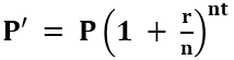
Where,
- P is the original principal sum
- P’ is the new principal sum
- n is the compounding frequency
- r is the nominal annual interest rate
- t is the overall length of the interest applied (expressed using the same time units as r, usually years).
Table of contents
- Compound Interest in Excel Formula
- How to Calculate Compound Interest in Excel Formula? (with Examples)
- Example #1 – Using Mathematical Compound Interest Excel Formula
- Example #2 – Using the Compound Interest Calculation Table in excel
- Example #3 – Compound Interest Using FVSCHEDULE Excel Formula
- Example #4 – Compound Interest Using the FV Excel Formula
- Things to Remember about Compound Interest Formula in Excel
- Recommended Articles
- How to Calculate Compound Interest in Excel Formula? (with Examples)
You are free to use this image on your website, templates, etc, Please provide us with an attribution linkArticle Link to be Hyperlinked
For eg:
Source: Compound Interest Formula in Excel (wallstreetmojo.com)
How to Calculate Compound Interest in Excel Formula? (with Examples)
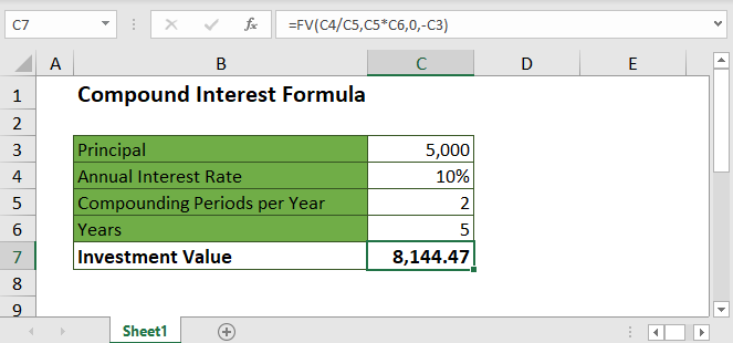
Let us understand the same using some examples of the Compound InterestTo calculate the compound interest in excel, the user can use the FV function and return the future value of an investment. To configure the function, the user must enter a rate, periods (time), the periodic payment, the present value. Compound interest formula = FV(rate,nper,pmt,pv)read more formula in Excel.
You can download this Compound Interest Excel Template here – Compound Interest Excel Template
Example #1 – Using Mathematical Compound Interest Excel Formula
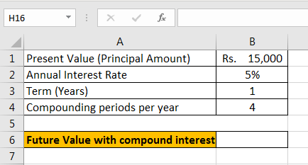
Suppose we have the following information to calculate compound interest in Excel.
It is like a compound interest calculator in Excel now. We can change the value for the annual interest rate, the number of years, and compounding periods per year as below.

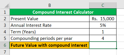
Example #2 – Using the Compound Interest Calculation Table in Excel
Suppose we have the following information to calculate compound interest in a table excel format (systematically).

Step 1 – We need to name cell E3 “Rate” by selecting the cell and changing the name using the “Name Box.“

Step 2 – We have the principal value or present value as ₹15,000, and the annual interest rate is 5%. To calculate the investment value at the end of quarter 1, we will add 5%/4, i.e., 1.25% interest, to the principal value.

The result is shown below:

Step 3 – We must drag the formula to the C6 cell by selecting the range C3:C6 and pressing “Ctrl+D.”
The future value after four quarters will be ₹15764.18.
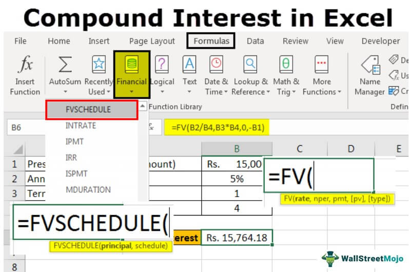
Example #3 – Compound Interest Using FVSCHEDULE Excel Formula
Suppose we have the following information to calculate compound interest in Excel.

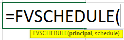
We will use the FVSCHEDULE function to calculate future valueThe Future Value (FV) formula is a financial terminology used to calculate cash flow value at a futuristic date compared to the original receipt. The objective of the FV equation is to determine the future value of a prospective investment and whether the returns yield sufficient returns to factor in the time value of money.read more. The FVSCHEDULE formula returns the future value of an initial principal after applying a series of compound interest rates.
To do the same, the steps are:
Step 1 – We will initiate writing the FVSCHEDULE function into cell B6. The function takes two arguments, i.e., principal and schedule.
- We need to give the amount we are investing in for the principal.
- We need to provide the list of interest rates with commas in curly braces for the schedule to calculate the value with compound interestCompound interest is the interest charged on the sum of the principal amount and the total interest amassed on it so far. It plays a crucial role in generating higher rewards from an investment.read more.
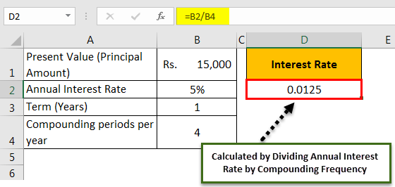
Step 2 – For ‘principal,’ we will provide the reference of the B1 cell, and for ‘schedule,’ we will specify 0.0125 as this is the value we get when we divide the 5% with 4.

The result is shown below:
Now, we can apply the FVSCHEDULE formula in Excel.

Step 3 – After pressing the Enter button, we get ₹15764.18 as the future value with compound interest in Excel.

Example #4 – Compound Interest Using the FV Excel Formula
Suppose we have the following data to calculate compound interest in Excel.
We will use the FV Excel formula to calculate compound interest.
FV function (stands for Future Value) returns the future value of an investment based on periodic, constant payments and a constant interest rate.
The syntax of the FV function is
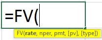
The argument in the FV function is:
- Rate: Rate is the constant interest rate per period in an annuity.
- Nper: Nper stands for the total number of periods in an annuity.
- Pmt: PMTPMT function is an advanced financial function to calculate the monthly payment against the simple loan amount. You have to provide basic information, including loan amount, interest rate, and duration of payment, and the function will calculate the payment as a result.read more stands for payment. It indicates the amount we will add to the annuity every period. If we omit this value, then it is mandatory to mention PV.
- PV: PV stands for present value. It is the amount which we are investing in. This amount is going out of our pocket, so by convention, this amount is mentioned with a negative sign.
- Type: This is an optional argument. We need to specify 0 if the amount is being added to the investment at the end of the period or one if the amount is being added to the investment at the beginning of the period.
We need to mention either the PMT or PV argument.
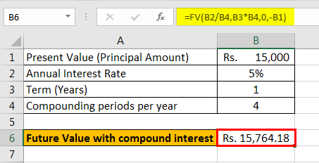
We will specify the rate as “Annual Interest Rate (B2)/ Compounding periods per year (B4).“

We need to specify nper as ‘Term (Years) * Compounding periods per year.’

As we will not add any additional amount to the principal value during the investment period, we will specify ‘0’ for “pmt.“

We have omitted the value for “pmt,“ and we are investing ₹15,000 as principal (present value). We will reference the B1 cell with a negative sign for “PV.”

After pressing the “Enter” button, we get ₹15764.18 as the future value with compound interest.
Things to Remember about Compound Interest Formula in Excel
- We need to insert the interest rate in percentage form (4%) or decimal form (0.04).
- As the “PMT” and “PV” arguments in the FV function outflows, in reality, we need to mention them in the negative form (with a minus (-) sign).
- FV function gives #VALUE! Error when any non-numeric value is provided as an argument.
- We need to mention either PMT or PV arguments in the FV function.
Recommended Articles
This article is a guide to Compound Interest in Excel. We discuss how to calculate compound interest in Excel, examples, and a downloadable Excel template. You may learn more about Excel from the following articles: –
- Formula of Monthly Compound Interest
- What is Quartile Formula?
- QUARTILE Function in Excel
- Excel NPER Function