Overview of formulas in Excel
Get started on how to create formulas and use built-in functions to perform calculations and solve problems.

Important: The calculated results of formulas and some Excel worksheet functions may differ slightly between a Windows PC using x86 or x86-64 architecture and a Windows RT PC using ARM architecture. Learn more about the differences.
Important: In this article we discuss XLOOKUP and VLOOKUP, which are similar. Try using the new XLOOKUP function, an improved version of VLOOKUP that works in any direction and returns exact matches by default, making it easier and more convenient to use than its predecessor.
Create a formula that refers to values in other cells
-
Select a cell.
-
Type the equal sign =.
Note: Formulas in Excel always begin with the equal sign.
-
Select a cell or type its address in the selected cell.

-
Enter an operator. For example, – for subtraction.
-
Select the next cell, or type its address in the selected cell.
-
Press Enter. The result of the calculation appears in the cell with the formula.


See a formula
-
When a formula is entered into a cell, it also appears in the Formula bar.
-
To see a formula, select a cell, and it will appear in the formula bar.


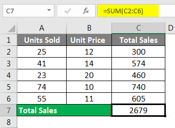
Enter a formula that contains a built-in function
-
Select an empty cell.
-
Type an equal sign = and then type a function. For example, =SUM for getting the total sales.
-
Type an opening parenthesis (.
-
Select the range of cells, and then type a closing parenthesis).
-
Press Enter to get the result.

Download our Formulas tutorial workbook
We’ve put together a Get started with Formulas workbook that you can download. If you’re new to Excel, or even if you have some experience with it, you can walk through Excel’s most common formulas in this tour. With real-world examples and helpful visuals, you’ll be able to Sum, Count, Average, and Vlookup like a pro.
Formulas in-depth
You can browse through the individual sections below to learn more about specific formula elements.
A formula can also contain any or all of the following: functions, references, operators, and constants.
Parts of a formula

1. Functions: The PI() function returns the value of pi: 3.142…
2. References: A2 returns the value in cell A2.
3. Constants: Numbers or text values entered directly into a formula, such as 2.
4. Operators: The ^ (caret) operator raises a number to a power, and the * (asterisk) operator multiplies numbers.
A constant is a value that is not calculated; it always stays the same. For example, the date 10/9/2008, the number 210, and the text «Quarterly Earnings» are all constants. An expression or a value resulting from an expression is not a constant. If you use constants in a formula instead of references to cells (for example, =30+70+110), the result changes only if you modify the formula. In general, it’s best to place constants in individual cells where they can be easily changed if needed, then reference those cells in formulas.
A reference identifies a cell or a range of cells on a worksheet, and tells Excel where to look for the values or data you want to use in a formula. You can use references to use data contained in different parts of a worksheet in one formula or use the value from one cell in several formulas. You can also refer to cells on other sheets in the same workbook, and to other workbooks. References to cells in other workbooks are called links or external references.
-
The A1 reference style
By default, Excel uses the A1 reference style, which refers to columns with letters (A through XFD, for a total of 16,384 columns) and refers to rows with numbers (1 through 1,048,576). These letters and numbers are called row and column headings. To refer to a cell, enter the column letter followed by the row number. For example, B2 refers to the cell at the intersection of column B and row 2.
To refer to
Use
The cell in column A and row 10
A10
The range of cells in column A and rows 10 through 20
A10:A20
The range of cells in row 15 and columns B through E
B15:E15
All cells in row 5
5:5
All cells in rows 5 through 10
5:10
All cells in column H
H:H
All cells in columns H through J
H:J
The range of cells in columns A through E and rows 10 through 20
A10:E20
-
Making a reference to a cell or a range of cells on another worksheet in the same workbook
In the following example, the AVERAGE function calculates the average value for the range B1:B10 on the worksheet named Marketing in the same workbook.
1. Refers to the worksheet named Marketing
2. Refers to the range of cells from B1 to B10
3. The exclamation point (!) Separates the worksheet reference from the cell range reference
Note: If the referenced worksheet has spaces or numbers in it, then you need to add apostrophes (‘) before and after the worksheet name, like =’123′!A1 or =’January Revenue’!A1.
-
The difference between absolute, relative and mixed references
-
Relative references A relative cell reference in a formula, such as A1, is based on the relative position of the cell that contains the formula and the cell the reference refers to. If the position of the cell that contains the formula changes, the reference is changed. If you copy or fill the formula across rows or down columns, the reference automatically adjusts. By default, new formulas use relative references. For example, if you copy or fill a relative reference in cell B2 to cell B3, it automatically adjusts from =A1 to =A2.
Copied formula with relative reference
-
Absolute references An absolute cell reference in a formula, such as $A$1, always refer to a cell in a specific location. If the position of the cell that contains the formula changes, the absolute reference remains the same. If you copy or fill the formula across rows or down columns, the absolute reference does not adjust. By default, new formulas use relative references, so you may need to switch them to absolute references. For example, if you copy or fill an absolute reference in cell B2 to cell B3, it stays the same in both cells: =$A$1.
Copied formula with absolute reference
-
Mixed references A mixed reference has either an absolute column and relative row, or absolute row and relative column. An absolute column reference takes the form $A1, $B1, and so on. An absolute row reference takes the form A$1, B$1, and so on. If the position of the cell that contains the formula changes, the relative reference is changed, and the absolute reference does not change. If you copy or fill the formula across rows or down columns, the relative reference automatically adjusts, and the absolute reference does not adjust. For example, if you copy or fill a mixed reference from cell A2 to B3, it adjusts from =A$1 to =B$1.
Copied formula with mixed reference
-
-
The 3-D reference style
Conveniently referencing multiple worksheets If you want to analyze data in the same cell or range of cells on multiple worksheets within a workbook, use a 3-D reference. A 3-D reference includes the cell or range reference, preceded by a range of worksheet names. Excel uses any worksheets stored between the starting and ending names of the reference. For example, =SUM(Sheet2:Sheet13!B5) adds all the values contained in cell B5 on all the worksheets between and including Sheet 2 and Sheet 13.
-
You can use 3-D references to refer to cells on other sheets, to define names, and to create formulas by using the following functions: SUM, AVERAGE, AVERAGEA, COUNT, COUNTA, MAX, MAXA, MIN, MINA, PRODUCT, STDEV.P, STDEV.S, STDEVA, STDEVPA, VAR.P, VAR.S, VARA, and VARPA.
-
3-D references cannot be used in array formulas.
-
3-D references cannot be used with the intersection operator (a single space) or in formulas that use implicit intersection.
What occurs when you move, copy, insert, or delete worksheets The following examples explain what happens when you move, copy, insert, or delete worksheets that are included in a 3-D reference. The examples use the formula =SUM(Sheet2:Sheet6!A2:A5) to add cells A2 through A5 on worksheets 2 through 6.
-
Insert or copy If you insert or copy sheets between Sheet2 and Sheet6 (the endpoints in this example), Excel includes all values in cells A2 through A5 from the added sheets in the calculations.
-
Delete If you delete sheets between Sheet2 and Sheet6, Excel removes their values from the calculation.
-
Move If you move sheets from between Sheet2 and Sheet6 to a location outside the referenced sheet range, Excel removes their values from the calculation.
-
Move an endpoint If you move Sheet2 or Sheet6 to another location in the same workbook, Excel adjusts the calculation to accommodate the new range of sheets between them.
-
Delete an endpoint If you delete Sheet2 or Sheet6, Excel adjusts the calculation to accommodate the range of sheets between them.
-
-
The R1C1 reference style
You can also use a reference style where both the rows and the columns on the worksheet are numbered. The R1C1 reference style is useful for computing row and column positions in macros. In the R1C1 style, Excel indicates the location of a cell with an «R» followed by a row number and a «C» followed by a column number.
Reference
Meaning
R[-2]C
A relative reference to the cell two rows up and in the same column
R[2]C[2]
A relative reference to the cell two rows down and two columns to the right
R2C2
An absolute reference to the cell in the second row and in the second column
R[-1]
A relative reference to the entire row above the active cell
R
An absolute reference to the current row
When you record a macro, Excel records some commands by using the R1C1 reference style. For example, if you record a command, such as clicking the AutoSum button to insert a formula that adds a range of cells, Excel records the formula by using R1C1 style, not A1 style, references.
You can turn the R1C1 reference style on or off by setting or clearing the R1C1 reference style check box under the Working with formulas section in the Formulas category of the Options dialog box. To display this dialog box, click the File tab.
Top of Page


Need more help?
You can always ask an expert in the Excel Tech Community or get support in the Answers community.
See Also
Switch between relative, absolute and mixed references for functions
Using calculation operators in Excel formulas
The order in which Excel performs operations in formulas
Using functions and nested functions in Excel formulas
Define and use names in formulas
Guidelines and examples of array formulas
Delete or remove a formula
How to avoid broken formulas
Find and correct errors in formulas
Excel keyboard shortcuts and function keys
Excel functions (by category)
Need more help?
Want more options?
Explore subscription benefits, browse training courses, learn how to secure your device, and more.
Communities help you ask and answer questions, give feedback, and hear from experts with rich knowledge.
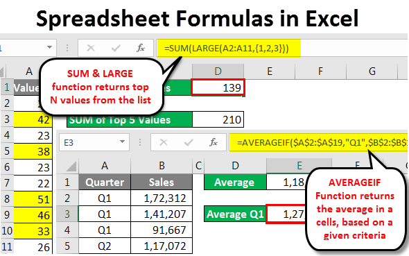
Table of Contents
- Spreadsheet Formulas in Excel
- How to Use Spreadsheet Formulas in Excel?
Spreadsheet Formulas in Excel
A spreadsheet is full of formulas. Firstly don’t get confused with the spreadsheet and worksheet; both are the same. This article will talk about the most important formulas in excel and how do we use them in our day-to-day activities.
How to Use Spreadsheet Formulas in Excel?
Spreadsheet Formulas in Excel are very simple and easy to use. This is the guide to Formulas in Excel with Detailed Spreadsheet Formulas Examples. Let’s understand how to use Spreadsheet Formulas in Excel with some examples.
You can download this Spreadsheet Formulas Excel Template here – Spreadsheet Formulas Excel Template
Example #1
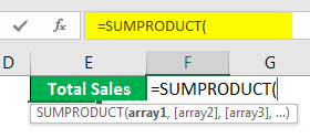
SUMPRODUCT Formula in Excel Spreadsheet
If we want to do unit price * unit sold calculation, we will do an individual calculation and finally add the total to get the total sales. For example, look at the below example.
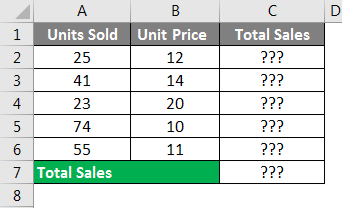
Firstly we calculate the total sales by multiplying Units Sold to Unit Price, as I have shown in the below image.
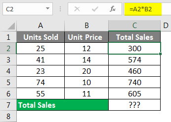
Finally, we add the total of sales to get the final total sales amount.
This includes many steps to get the final sales amount. However, using the SUMPRODUCT function, we can get the total in a single formula itself.
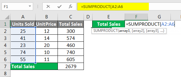
In the first array, select Units Sold range.
We need to do the multiplication, so enter an asterisk (*) symbol and select Unit Price.
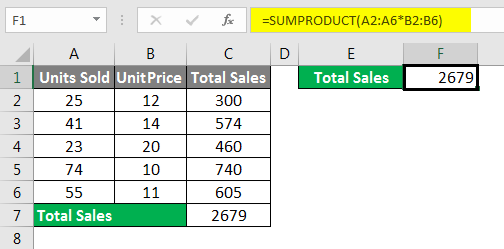
Oh yes, we got our end result in a single formula in a single cell itself. How cool is it?
Example #2
Formula to SUM Top N Values in Excel Spreadsheet
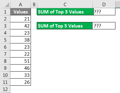
We all work on the SUM function in Excel Spreadsheet in Excel day in day out in an Excel Spreadsheet; this is not a strange thing for us. But how do we sum the top 3 values or top 5 values, or top X values?
It looks like a new thing isn’t it? Yes, we can SUM Top N values from the list. For example, look at the below data.
With the combination of SUM & LARGE function in an Excel Spreadsheet, we can sum the top n values from the list. The LARGE function helps us to find the top largest value.
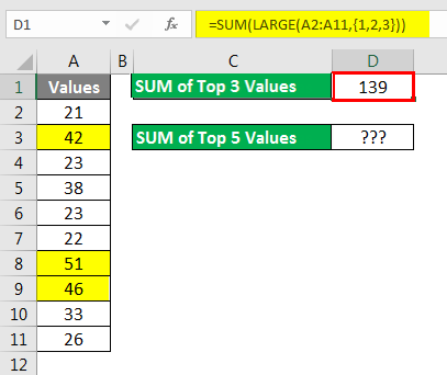
In order to find the top 3 values, I applied the SUM function formula for this SUM function. I have entered one more function, LARGE, to get the top N values. A LARGE function in Excel Spreadsheet can return only one largest in order to find the top N values. We need to supply the numbers in curly brackets ({). Now LARGE will return the top 3 largest values, and the SUM function will add these 3 numbers and give us the total.
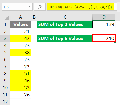
Similarly, if I want the sum of the top 5 values from the list in the Excel Spreadsheet, I need to supply the numbers to 5 in curly brackets. Now LARGE will return the top 5 largest values, and the SUM function will add these 5 numbers and give the total.
Example #3
SUMIF Formula with Operator Symbols in Excel Spreadsheet
You must have worked with the SUMIF function while using Excel Spreadsheet, and you are perfectly alright as well. But we can pass the criteria to the SUMIF function formula with operator symbol as well. For an example, look at the below example.
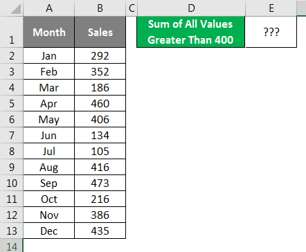
We need to do the addition of all the values which are greater than 400. For sure, we need to use the SUMIF function, but in criteria, we need to supply an operator symbol greater than (>) and mention the criteria as 400.
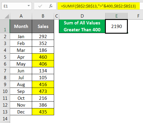
Yes, we need to supply the criteria operator symbol in double quotes (” “) and combine the other criteria with the ampersand (&) symbol. Now formula will read it as greater than 400 and returns the total.
I have marked all the values which are greater than 400 with yellow color; you can add those values manually you will get the same total as 2190.
Example #4
Table for All kind of Calculations in Excel Spreadsheet
Often we need to do the summation of values; often, we need the count, often the Average of the numbers, and many other things. How do you deal with all these requirements in a single formula?
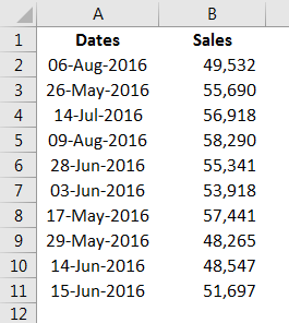
Assume below is the data you have in your Excel Spreadsheet.
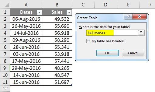
Step 1: Convert this range to the table by pressing Ctrl + T.
Step 2: Place a cursor inside the table > go to Design > Under Table Style Options check the option Total Row.
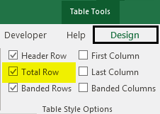
Step 3: Now, we have a total of the table row at the end of the table.
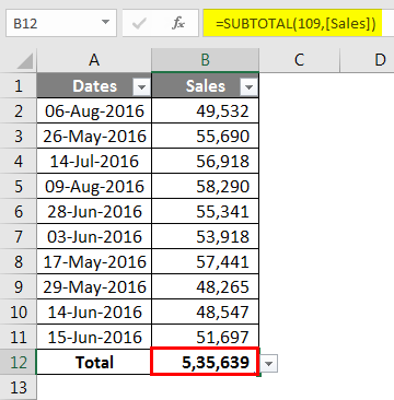
Step 4: But if you observe, it is not the only formula; rather, it has a drop-down list. Click on the drop-down list to see what more has in it.
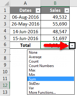
Using this drop-down, we can use Average, Count, find the Max value, find the Min value, and many other things as well. Based on the selection we make from the drop-down, it will show the results.
Example #5
AVERAGEIF Formula in Excel Spreadsheet
AVERAGE function is not a strange thing for us. At the point of time, if we need the average of values, we would apply the AVERAGE function formula in Excel Spreadsheet and get the result. For example, if I need the average of the below numbers, I would apply the AVERAGE function.
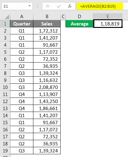
What if we need an Average only for the quarter Q1? How do we do? We can do with manual work, but we all hate manual work isn’t it?
Nothing to worry about; we have a function called AVERAGEIF in Excel Spreadsheet.
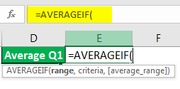
The range is nothing but our Quarter Range, so select Quarter range from A2 to A19.
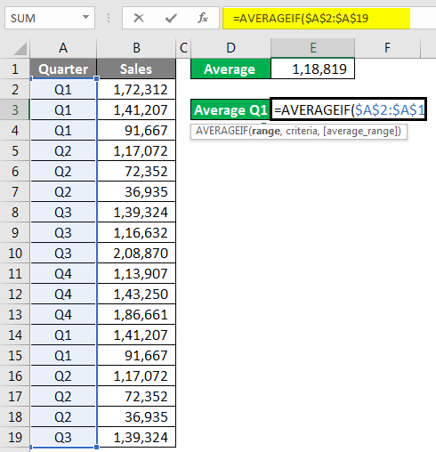
Criteria are what you want to do from this range. Our criteria are Q1.
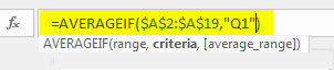
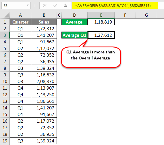
The average Range is nothing but the sales column to select the Sales column and close the bracket. We will get Q1 Average Only.
Example #6
IFERROR Formula to Avoid Errors in Excel Spreadsheet
I am sure you have encountered many errors while applying formulas. Often times we need to ignore these errors and clear these error values as per our own values. For example, look at the below illustrations.
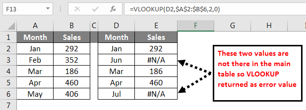
In the above image, we got error values. I want to convert all the error values to Not Found. Apply the below formula to get the result.
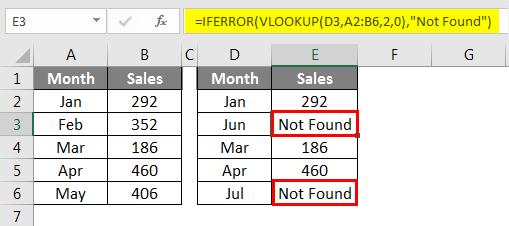
If VLOOKUP returns an error values IFERROR convert this to Not Found text value.
Example #7
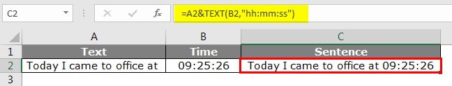
TEXT Function to Concatenate Date Values in Excel Spreadsheet
Using CONCATENATE function, we can combine many cell data into one. But this does not work a similar way if you are combining dates with text in Excel Spreadsheet. Look at the below image.
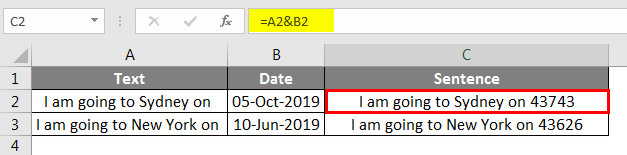
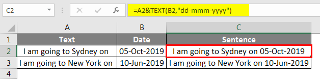
When I combined cells A1 & A2, I got the result of these two cell values. However, a date is not in the correct format; in order to make this a perfect format, we need to use the TEXT function to apply our date format.
Below is the formula which can make this a proper sentence.
Example #8
TEXT Function to Concatenate Time Values in Excel Spreadsheet
Like how we got an incorrect format for date similarly for time format, also we get incorrect format.
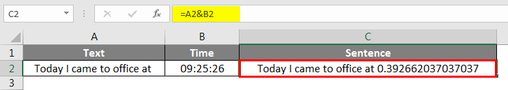
We need to pass the time cell with the TEXT function and convert it to “hh:mm:ss” format in Excel Spreadsheet.
Things to Remember
- Using CONCATENATE function, we can combine many cell data into one.
- In order to make the Date Format correct, we need to use the TEXT function to apply our date format.
- By using the SUMPRODUCT function, we can get the total in the single formula itself.
Recommended Articles
This has been a guide to Spreadsheet Formulas in Excel. Here we discussed different Spreadsheet formulas in Excel, How to use Spreadsheet Formulas in Excel, along with practical examples and downloadable excel template. You can also go through our other suggested articles-
- Advanced Formulas in Excel
- Excel Spreadsheet Examples
- Create Spreadsheet in Excel
- Worksheets in Excel
Formulas and functions are the building blocks of working with numeric data in Excel. This article introduces you to formulas and functions.
In this article, we will cover the following topics.
- What is Formulas in Excel?
- Mistakes to avoid when working with formulas in Excel
- What is Function in Excel?
- The importance of functions
- Common functions
- Numeric Functions
- String functions
- Date Time functions
- V Lookup function
Tutorials Data
For this tutorial, we will work with the following datasets.
Home supplies budget
| S/N | ITEM | QTY | PRICE | SUBTOTAL | Is it Affordable? |
|---|---|---|---|---|---|
| 1 | Mangoes | 9 | 600 | ||
| 2 | Oranges | 3 | 1200 | ||
| 3 | Tomatoes | 1 | 2500 | ||
| 4 | Cooking Oil | 5 | 6500 | ||
| 5 | Tonic Water | 13 | 3900 |
House Building Project Schedule
| S/N | ITEM | START DATE | END DATE | DURATION (DAYS) |
|---|---|---|---|---|
| 1 | Survey land | 04/02/2015 | 07/02/2015 | |
| 2 | Lay Foundation | 10/02/2015 | 15/02/2015 | |
| 3 | Roofing | 27/02/2015 | 03/03/2015 | |
| 4 | Painting | 09/03/2015 | 21/03/2015 |
What is Formulas in Excel?
FORMULAS IN EXCEL is an expression that operates on values in a range of cell addresses and operators. For example, =A1+A2+A3, which finds the sum of the range of values from cell A1 to cell A3. An example of a formula made up of discrete values like =6*3.
=A2 * D2 / 2
HERE,
"="tells Excel that this is a formula, and it should evaluate it."A2" * D2"makes reference to cell addresses A2 and D2 then multiplies the values found in these cell addresses."/"is the division arithmetic operator"2"is a discrete value
Formulas practical exercise
We will work with the sample data for the home budget to calculate the subtotal.
- Create a new workbook in Excel
- Enter the data shown in the home supplies budget above.
- Your worksheet should look as follows.

We will now write the formula that calculates the subtotal
Set the focus to cell E4
Enter the following formula.
=C4*D4
HERE,
"C4*D4"uses the arithmetic operator multiplication (*) to multiply the value of the cell address C4 and D4.
Press enter key
You will get the following result

The following animated image shows you how to auto select cell address and apply the same formula to other rows.

Mistakes to avoid when working with formulas in Excel
- Remember the rules of Brackets of Division, Multiplication, Addition, & Subtraction (BODMAS). This means expressions are brackets are evaluated first. For arithmetic operators, the division is evaluated first followed by multiplication then addition and subtraction is the last one to be evaluated. Using this rule, we can rewrite the above formula as =(A2 * D2) / 2. This will ensure that A2 and D2 are first evaluated then divided by two.
- Excel spreadsheet formulas usually work with numeric data; you can take advantage of data validation to specify the type of data that should be accepted by a cell i.e. numbers only.
- To ensure that you are working with the correct cell addresses referenced in the formulas, you can press F2 on the keyboard. This will highlight the cell addresses used in the formula, and you can cross check to ensure they are the desired cell addresses.
- When you are working with many rows, you can use serial numbers for all the rows and have a record count at the bottom of the sheet. You should compare the serial number count with the record total to ensure that your formulas included all the rows.
Check Out
Top 10 Excel Spreadsheet Formulas
What is Function in Excel?
FUNCTION IN EXCEL is a predefined formula that is used for specific values in a particular order. Function is used for quick tasks like finding the sum, count, average, maximum value, and minimum values for a range of cells. For example, cell A3 below contains the SUM function which calculates the sum of the range A1:A2.
- SUM for summation of a range of numbers
- AVERAGE for calculating the average of a given range of numbers
- COUNT for counting the number of items in a given range
The importance of functions
Functions increase user productivity when working with excel. Let’s say you would like to get the grand total for the above home supplies budget. To make it simpler, you can use a formula to get the grand total. Using a formula, you would have to reference the cells E4 through to E8 one by one. You would have to use the following formula.
= E4 + E5 + E6 + E7 + E8
With a function, you would write the above formula as
=SUM (E4:E8)
As you can see from the above function used to get the sum of a range of cells, it is much more efficient to use a function to get the sum than using the formula which will have to reference a lot of cells.
Common functions
Let’s look at some of the most commonly used functions in ms excel formulas. We will start with statistical functions.
| S/N | FUNCTION | CATEGORY | DESCRIPTION | USAGE |
|---|---|---|---|---|
| 01 | SUM | Math & Trig | Adds all the values in a range of cells | =SUM(E4:E8) |
| 02 | MIN | Statistical | Finds the minimum value in a range of cells | =MIN(E4:E8) |
| 03 | MAX | Statistical | Finds the maximum value in a range of cells | =MAX(E4:E8) |
| 04 | AVERAGE | Statistical | Calculates the average value in a range of cells | =AVERAGE(E4:E8) |
| 05 | COUNT | Statistical | Counts the number of cells in a range of cells | =COUNT(E4:E8) |
| 06 | LEN | Text | Returns the number of characters in a string text | =LEN(B7) |
| 07 | SUMIF | Math & Trig |
Adds all the values in a range of cells that meet a specified criteria. =SUMIF(range,criteria,[sum_range]) |
=SUMIF(D4:D8,”>=1000″,C4:C8) |
| 08 | AVERAGEIF | Statistical |
Calculates the average value in a range of cells that meet the specified criteria. =AVERAGEIF(range,criteria,[average_range]) |
=AVERAGEIF(F4:F8,”Yes”,E4:E8) |
| 09 | DAYS | Date & Time | Returns the number of days between two dates | =DAYS(D4,C4) |
| 10 | NOW | Date & Time | Returns the current system date and time | =NOW() |
Numeric Functions
As the name suggests, these functions operate on numeric data. The following table shows some of the common numeric functions.
| S/N | FUNCTION | CATEGORY | DESCRIPTION | USAGE |
|---|---|---|---|---|
| 1 | ISNUMBER | Information | Returns True if the supplied value is numeric and False if it is not numeric | =ISNUMBER(A3) |
| 2 | RAND | Math & Trig | Generates a random number between 0 and 1 | =RAND() |
| 3 | ROUND | Math & Trig | Rounds off a decimal value to the specified number of decimal points | =ROUND(3.14455,2) |
| 4 | MEDIAN | Statistical | Returns the number in the middle of the set of given numbers | =MEDIAN(3,4,5,2,5) |
| 5 | PI | Math & Trig | Returns the value of Math Function PI(π) | =PI() |
| 6 | POWER | Math & Trig |
Returns the result of a number raised to a power. POWER( number, power ) |
=POWER(2,4) |
| 7 | MOD | Math & Trig | Returns the Remainder when you divide two numbers | =MOD(10,3) |
| 8 | ROMAN | Math & Trig | Converts a number to roman numerals | =ROMAN(1984) |
String functions
These basic excel functions are used to manipulate text data. The following table shows some of the common string functions.
| S/N | FUNCTION | CATEGORY | DESCRIPTION | USAGE | COMMENT |
|---|---|---|---|---|---|
| 1 | LEFT | Text | Returns a number of specified characters from the start (left-hand side) of a string | =LEFT(“GURU99”,4) | Left 4 Characters of “GURU99” |
| 2 | RIGHT | Text | Returns a number of specified characters from the end (right-hand side) of a string | =RIGHT(“GURU99”,2) | Right 2 Characters of “GURU99” |
| 3 | MID | Text |
Retrieves a number of characters from the middle of a string from a specified start position and length. =MID (text, start_num, num_chars) |
=MID(“GURU99”,2,3) | Retrieving Characters 2 to 5 |
| 4 | ISTEXT | Information | Returns True if the supplied parameter is Text | =ISTEXT(value) | value – The value to check. |
| 5 | FIND | Text |
Returns the starting position of a text string within another text string. This function is case-sensitive. =FIND(find_text, within_text, [start_num]) |
=FIND(“oo”,”Roofing”,1) | Find oo in “Roofing”, Result is 2 |
| 6 | REPLACE | Text |
Replaces part of a string with another specified string. =REPLACE (old_text, start_num, num_chars, new_text) |
=REPLACE(“Roofing”,2,2,”xx”) | Replace “oo” with “xx” |
Date Time Functions
These functions are used to manipulate date values. The following table shows some of the common date functions
| S/N | FUNCTION | CATEGORY | DESCRIPTION | USAGE |
|---|---|---|---|---|
| 1 | DATE | Date & Time | Returns the number that represents the date in excel code | =DATE(2015,2,4) |
| 2 | DAYS | Date & Time | Find the number of days between two dates | =DAYS(D6,C6) |
| 3 | MONTH | Date & Time | Returns the month from a date value | =MONTH(“4/2/2015”) |
| 4 | MINUTE | Date & Time | Returns the minutes from a time value | =MINUTE(“12:31”) |
| 5 | YEAR | Date & Time | Returns the year from a date value | =YEAR(“04/02/2015”) |
VLOOKUP function
The VLOOKUP function is used to perform a vertical look up in the left most column and return a value in the same row from a column that you specify. Let’s explain this in a layman’s language. The home supplies budget has a serial number column that uniquely identifies each item in the budget. Suppose you have the item serial number, and you would like to know the item description, you can use the VLOOKUP function. Here is how the VLOOKUP function would work.

=VLOOKUP (C12, A4:B8, 2, FALSE)
HERE,
"=VLOOKUP"calls the vertical lookup function"C12"specifies the value to be looked up in the left most column"A4:B8"specifies the table array with the data"2"specifies the column number with the row value to be returned by the VLOOKUP function"FALSE,"tells the VLOOKUP function that we are looking for an exact match of the supplied look up value
The animated image below shows this in action

Download the above Excel Code
Summary
Excel allows you to manipulate the data using formulas and/or functions. Functions are generally more productive compared to writing formulas. Functions are also more accurate compared to formulas because the margin of making mistakes is very minimum.
Here is a list of important Excel Formula and Function
- SUM function =
=SUM(E4:E8)
- MIN function =
=MIN(E4:E8)
- MAX function =
=MAX(E4:E8)
- AVERAGE function =
=AVERAGE(E4:E8)
- COUNT function =
=COUNT(E4:E8)
- DAYS function =
=DAYS(D4,C4)
- VLOOKUP function =
=VLOOKUP (C12, A4:B8, 2, FALSE)
- DATE function =
=DATE(2020,2,4)
Asked by: Miss Eloisa Nitzsche
Score: 4.6/5
(39 votes)
Create a simple formula in Excel
- On the worksheet, click the cell in which you want to enter the formula.
- Type the = (equal sign) followed by the constants and operators (up to 8192 characters) that you want to use in the calculation. For our example, type =1+1. Notes: …
- Press Enter (Windows) or Return (Mac).
What is the formula for spreadsheet?
A formula is an equation that makes calculations based on the data in your spreadsheet. Formulas are entered into a cell in your worksheet. They must begin with an equal sign, followed by the addresses of the cells that will be calculated upon, with an appropriate operand placed in between.
What are the 5 functions in Excel?
5 Functions of Excel/Sheets That Every Professional Should Know
- VLookup Formula.
- Concatenate Formula.
- Text to Columns.
- Remove Duplicates.
- Pivot Tables.
What are basic Excel skills?
These basic Excel skills are – familiarity with Excel ribbons & UI, ability to enter and format data, calculate totals & summaries thru formulas, highlight data that meets certain conditions, creating simple reports & charts, understanding the importance of keyboard shortcuts & productivity tricks.
What are the 3 common uses for Excel?
The three most common general uses for spreadsheet software are to create budgets, produce graphs and charts, and for storing and sorting data. Within business spreadsheet software is used to forecast future performance, calculate tax, completing basic payroll, producing charts and calculating revenues.
35 related questions found
How do I create a formula for a column in Excel?
Create a calculated column
- Create a table. …
- Insert a new column into the table. …
- Type the formula that you want to use, and press Enter. …
- When you press Enter, the formula is automatically filled into all cells of the column — above as well as below the cell where you entered the formula.
What are the basic Excel formulas?
Seven Basic Excel Formulas For Your Workflow
- =SUM(number1, [number2], …) …
- =SUM(A2:A8) – A simple selection that sums the values of a column.
- =SUM(A2:A8)/20 – Shows you can also turn your function into a formula. …
- =AVERAGE(number1, [number2], …) …
- =AVERAGE(B2:B11) – Shows a simple average, also similar to (SUM(B2:B11)/10)
How do you create a formula in Excel?
How to do calculations in Excel
- Type the equal symbol (=) in a cell. This tells Excel that you are entering a formula, not just numbers.
- Type the equation you want to calculate. For example, to add up 5 and 7, you type =5+7.
- Press the Enter key to complete your calculation. Done!
How do I apply one formula to all cells in Excel?
Simply do the following:
- Select the cell with the formula and the adjacent cells you want to fill.
- Click Home > Fill, and choose either Down, Right, Up, or Left. Keyboard shortcut: You can also press Ctrl+D to fill the formula down in a column, or Ctrl+R to fill the formula to the right in a row.
How do I create a simple Excel spreadsheet?
Step 1: Open MS Excel. Step 2: Go to Menu and select New >> click on the Blank workbook to create a simple worksheet. OR – Just press Ctrl + N: To create a new spreadsheet. Step 3: Go to the spreadsheet work area.
What is basic formula?
Formula is an expression that calculates values in a cell or in a range of cells. For example, =A2+A2+A3+A4 is a formula that adds up the values in cells A2 through A4. Function is a predefined formula already available in Excel.
What is Excel used for?
What is Excel used for? Excel is typically used to organize data and perform financial analysis. It is used across all business functions and at companies from small to large.
What is the best way to learn Excel?
5 Tips for Learning Excel
- Practice Simple Math Problems in Excel. When it comes to Excel, it’s easiest to start with basic math. …
- Learn How to Create Tables. …
- Learn How to Create Charts. …
- Take Excel Training Courses. …
- Earn a Microsoft Office Specialist Certification.
What is spreadsheet example?
Examples of spreadsheet programs
- Google Sheets — (online and free).
- iWork Numbers — Apple Office Suite.
- LibreOffice -> Calc (free).
- Lotus 1-2-3 (discontinued).
- Lotus Symphony — Spreadsheets.
- Microsoft Excel.
- OpenOffice -> Calc (free).
- VisiCalc (discontinued).
Which software is used for spreadsheet?
By far, the most frequently used spreadsheet program is Microsoft Excel, but other spreadsheet applications exist as well. Examples include: Lotus 1-2-3, Microsoft Works Spreadsheet, Open Office Calc and Google Drive Spreadsheet.
How many formulas are in Excel?
Excel has over 475 formulas in its Functions Library, from simple mathematics to very complex statistical, logical, and engineering tasks such as IF statements (one of our perennial favorite stories); AND, OR, NOT functions; COUNT, AVERAGE, and MIN/MAX.
How do I make a good Excel spreadsheet?
Excel for Architects – 9 Steps to Beautiful Spreadsheets
- Choose a good font. …
- Align your data. …
- Give your data some space. …
- Define your headers. …
- Choose your colors carefully. …
- Shade alternate rows for readability. …
- Use Grids Sparingly. …
- Create cell styles for consistency.
How do I format a spreadsheet in Excel?
Formatting text and numbers
- Select the cells(s) you want to modify. Selecting a cell range.
- Click the drop-down arrow next to the Number Format command on the Home tab. The Number Formatting drop-down menu will appear.
- Select the desired formatting option. …
- The selected cells will change to the new formatting style.
How do you create a worksheet?
How to create a worksheet template
- Select the worksheet that you want to use as a template.
- Click the File tab.
- Under Info, click Save As.
- In the File name box, type the name of the worksheet template. To create a custom worksheet template, type the file name that you want to use. …
- Do one of the following: …
- Click Save.
How do I write an if statement in Excel?
Use the IF function, one of the logical functions, to return one value if a condition is true and another value if it’s false. For example: =IF(A2>B2,»Over Budget»,»OK») =IF(A2=B2,B4-A4,»»)
What are the shortcuts in Excel?
Microsoft Excel keyboard shortcuts
- Ctrl + N: To create a new workbook.
- Ctrl + O: To open a saved workbook.
- Ctrl + S: To save a workbook.
- Ctrl + A: To select all the contents in a workbook.
- Ctrl + B: To turn highlighted cells bold.
- Ctrl + C: To copy cells that are highlighted.
- Ctrl + D:
Excel formulas allow you to identify relationships between values in your spreadsheet’s cells, perform mathematical calculations with those values, and return the resulting value in the cell of your choice. Sum, subtraction, percentage, division, average, and even dates/times are among the formulas that can be performed automatically. For example, =A1+A2+A3+A4+A5, which finds the sum of the range of values from cell A1 to cell A5.
Excel Functions: A formula is a mathematical expression that computes the value of a cell. Functions are predefined formulas that are already in Excel. Functions carry out specific calculations in a specific order based on the values specified as arguments or parameters. For example, =SUM (A1:A10). This function adds up all the values in cells A1 through A10.
How to Insert Formulas in Excel?
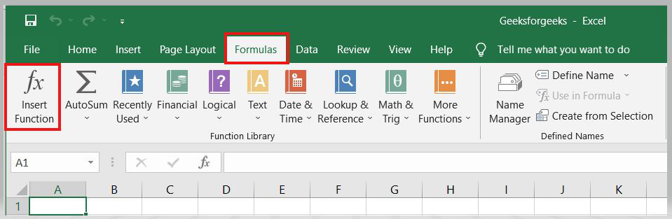
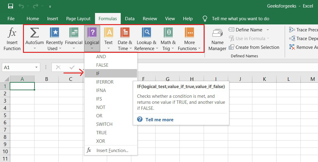
This horizontal menu, shown below, in more recent versions of Excel allows you to find and insert Excel formulas into specific cells of your spreadsheet. On the Formulas tab, you can find all available Excel functions in the Function Library:
The more you use Excel formulas, the easier it will be to remember and perform them manually. Excel has over 400 functions, and the number is increasing from version to version. The formulas can be inserted into Excel using the following method:
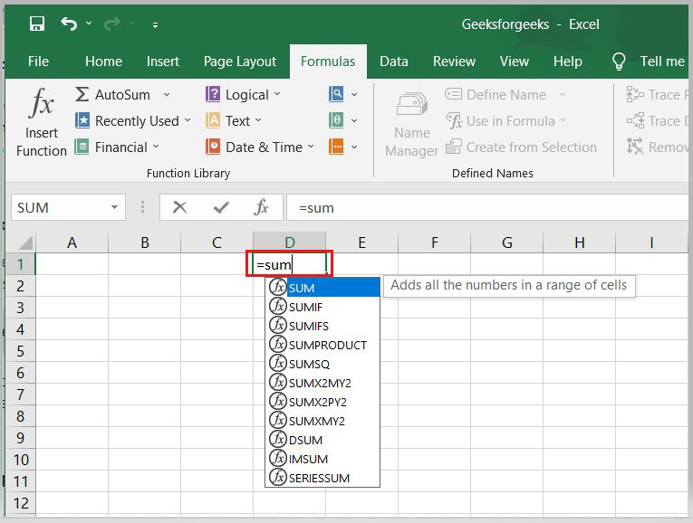
1. Simple insertion of the formula(Typing a formula in the cell):
Typing a formula into a cell or the formula bar is the simplest way to insert basic Excel formulas. Typically, the process begins with typing an equal sign followed by the name of an Excel function. Excel is quite intelligent in that it displays a pop-up function hint when you begin typing the name of the function.
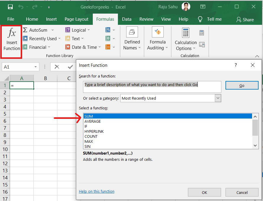
2. Using the Insert Function option on the Formulas Tab:
If you want complete control over your function insertion, use the Excel Insert Function dialogue box. To do so, go to the Formulas tab and select the first menu, Insert Function. All the functions will be available in the dialogue box.
3. Choosing a Formula from One of the Formula Groups in the Formula Tab:
This option is for those who want to quickly dive into their favorite functions. Navigate to the Formulas tab and select your preferred group to access this menu. Click to reveal a sub-menu containing a list of functions. You can then choose your preference. If your preferred group isn’t on the tab, click the More Functions option — it’s most likely hidden there.
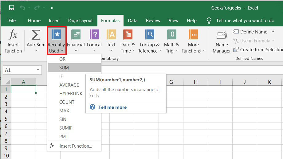
4. Use Recently Used Tabs for Quick Insertion:
If retyping your most recent formula becomes tedious, use the Recently Used menu. It’s on the Formulas tab, the third menu option after AutoSum.
Basic Excel Formulas and Functions:
1. SUM:
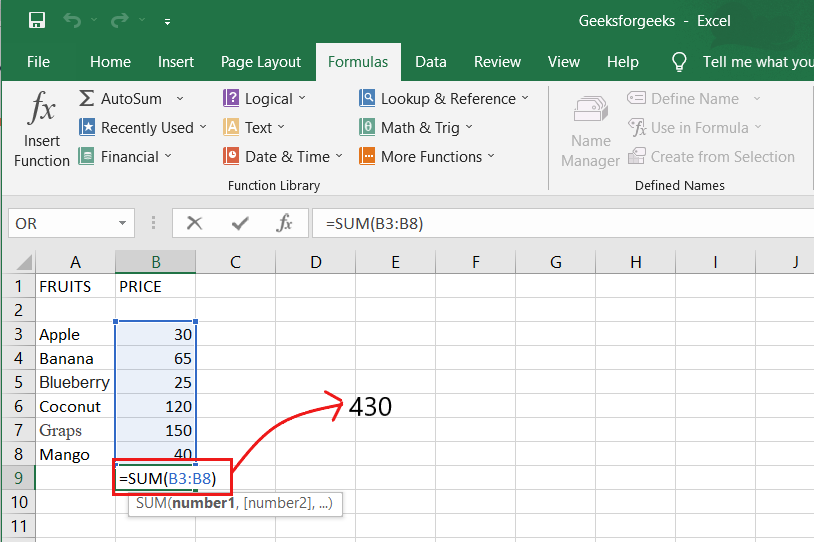
The SUM formula in Excel is one of the most fundamental formulas you can use in a spreadsheet, allowing you to calculate the sum (or total) of two or more values. To use the SUM formula, enter the values you want to add together in the following format: =SUM(value 1, value 2,…..).
Example: In the below example to calculate the sum of price of all the fruits, in B9 cell type =SUM(B3:B8). this will calculate the sum of B3, B4, B5, B6, B7, B8 Press “Enter,” and the cell will produce the sum: 430.
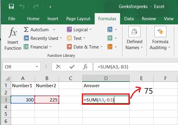
2. SUBTRACTION:
To use the subtraction formula in Excel, enter the cells you want to subtract in the format =SUM (A1, -B1). This will subtract a cell from the SUM formula by appending a negative sign before the cell being subtracted.
For example, if A3 was 300 and B3 was 225, =SUM(A1, -B1) would perform 300 + -225, returning a value of 75 in D3 cell.
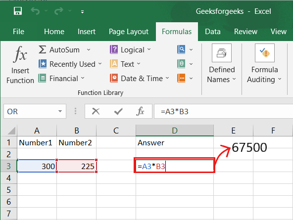
3. MULTIPLICATION:
In Excel, enter the cells to be multiplied in the format =A3*B3 to perform the multiplication formula. An asterisk is used in this formula to multiply cell A3 by cell B3.
For example, if A3 was 300 and B3 was 225, =A1*B1 would return a value of 67500.
Highlight an empty cell in an Excel spreadsheet to multiply two or more values. Then, in the format =A1*B1…, enter the values or cells you want to multiply together. The asterisk effectively multiplies each value in the formula.
To return your desired product, press Enter. Take a look at the screenshot above to see how this looks.
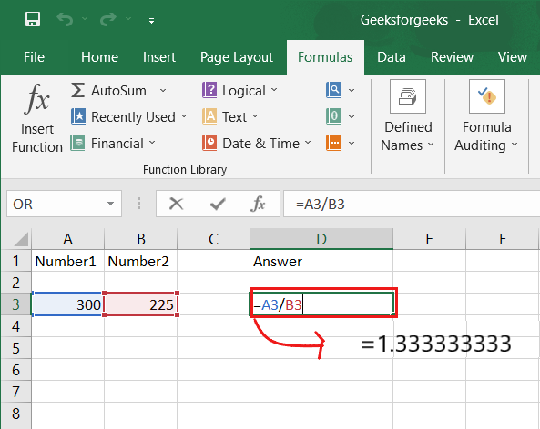
4. DIVISION:
To use the division formula in Excel, enter the dividing cells in the format =A3/B3. This formula divides cell A3 by cell B3 with a forward slash, “/.”
For example, if A3 was 300 and B3 was 225, =A3/B3 would return a decimal value of 1.333333333.
Division in Excel is one of the most basic functions available. To do so, highlight an empty cell, enter an equals sign, “=,” and then the two (or more) values you want to divide, separated by a forward slash, “/.” The output should look like this: =A3/B3, as shown in the screenshot above.
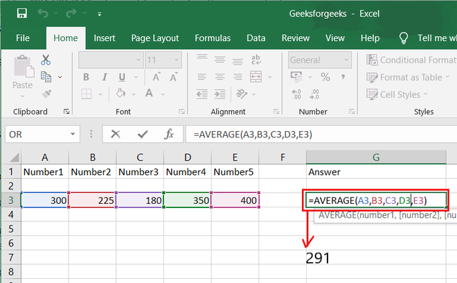
5. AVERAGE:
The AVERAGE function finds an average or arithmetic mean of numbers. to find the average of the numbers type = AVERAGE(A3.B3,C3….) and press ‘Enter’ it will produce average of the numbers in the cell.
For example, if A3 was 300, B3 was 225, C3 was 180, D3 was 350, E3 is 400 then =AVERAGE(A3,B3,C3,D3,E3) will produce 291.
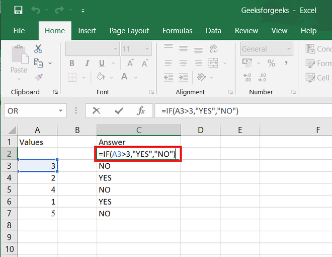
6. IF formula:
In Excel, the IF formula is denoted as =IF(logical test, value if true, value if false). This lets you enter a text value into a cell “if” something else in your spreadsheet is true or false.
For example, You may need to know which values in column A are greater than three. Using the =IF formula, you can quickly have Excel auto-populate a “yes” for each cell with a value greater than 3 and a “no” for each cell with a value less than 3.
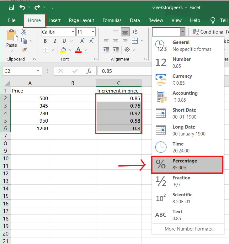
7. PERCENTAGE:
To use the percentage formula in Excel, enter the cells you want to calculate the percentage for in the format =A1/B1. To convert the decimal value to a percentage, select the cell, click the Home tab, and then select “Percentage” from the numbers dropdown.
There isn’t a specific Excel “formula” for percentages, but Excel makes it simple to convert the value of any cell into a percentage so you don’t have to calculate and reenter the numbers yourself.
The basic setting for converting a cell’s value to a percentage is found on the Home tab of Excel. Select this tab, highlight the cell(s) you want to convert to a percentage, and then select Conditional Formatting from the dropdown menu (this menu button might say “General” at first). Then, from the list of options that appears, choose “Percentage.” This will convert the value of each highlighted cell into a percentage. This feature can be found further down.
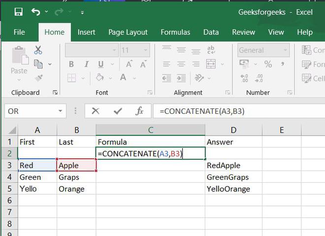
8. CONCATENATE:
CONCATENATE is a useful formula that combines values from multiple cells into the same cell.
For example , =CONCATENATE(A3,B3) will combine Red and Apple to produce RedApple.
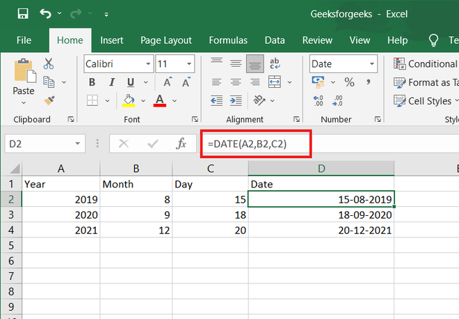
9. DATE:
DATE is the Excel DATE formula =DATE(year, month, day). This formula will return a date corresponding to the values entered in the parentheses, including values referred to from other cells.. For example, if A2 was 2019, B2 was 8, and C1 was 15, =DATE(A1,B1,C1) would return 15-08-2019.
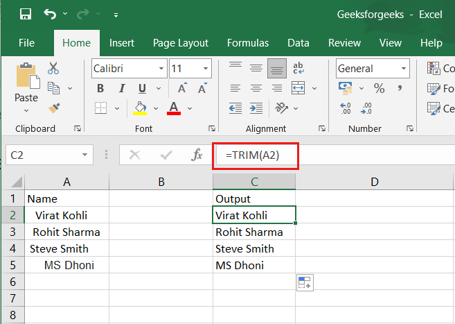
10. TRIM:
The TRIM formula in Excel is denoted =TRIM(text). This formula will remove any spaces that have been entered before and after the text in the cell. For example, if A2 includes the name ” Virat Kohli” with unwanted spaces before the first name, =TRIM(A2) would return “Virat Kohli” with no spaces in a new cell.
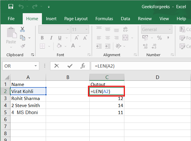
11. LEN:
LEN is the function to count the number of characters in a specific cell when you want to know the number of characters in that cell. =LEN(text) is the formula for this. Please keep in mind that the LEN function in Excel counts all characters, including spaces:
For example,=LEN(A2), returns the total length of the character in cell A2 including spaces.